Mar 12, 2018 - branching processes: the role of summary statistics .... of our current approach is the inclusion of a summary statistic in the development of.
arXiv:1803.04235v1 [stat.ME] 12 Mar 2018
Approximate Bayesian Computation in controlled branching processes: the role of summary statistics M. Gonz´alez, R. Mart´ınez, C. Minuesa, I. del Puerto March 13, 2018
Abstract Controlled branching processes are stochastic growth population models in which the number of individuals with reproductive capacity in each generation is controlled by a random control function. The purpose of this work is to examine the Approximate Bayesian Computation (ABC) methods and to propose appropriate summary statistics for them in the context of these processes. This methodology enables to approximate the posterior distribution of the parameters of interest satisfactorily without explicit likelihood calculations and under a minimal set of assumptions. In particular, the tolerance rejection algorithm, the sequential Monte Carlo ABC algorithm, and a post-sampling correction method based on local-linear regression are provided. The accuracy of the proposed methods are illustrated and compared with a “likelihood free” Markov chain Monte Carlo technique by the way of a simulated example developed with the statistical software R.
1
Introduction
Controlled branching processes are a family of discrete-time stochastic processes which are appropriate to describe population dynamics. In this model, as a generalization of the standard branching process - the so-called Bienaym´e-Galton-Watson process-, each individual reproduces independently of the others and following the same distribution, referred as the offspring law. The novelty of the controlled branching process (CBP) lies in the presence of a mechanism establishing the number of individuals with reproductive capacity (progenitors) in each generation. Thus, the evolution of populations suffering from the existence of predators, populations of invasive species or different migratory movements can be modelled by using this branching process (see Gonz´alez, Minuesa, and del Puerto (2017) for further details). The nature of this control mechanism can be either deterministic or random - described in this latter case by what are referred as control laws
1
-, giving rise to the models introduced by Sevast’yanov and Zubkov (1974) and Yanev (1975), respectively. The recent monograph Gonz´alez, del Puerto, and Yanev (2018) provides an extensive description of the probabilistic theory and inferential issues of CBPs. Due to the fact that the behaviour of these processes is determined by the parameters of the model associated to the offspring and control laws, and in real situations, those values are unknown, the research on statistical procedures that provide information about them is of great interest. Focusing the attention mainly on a Bayesian outlook, one can find the papers Mart´ınez, Mota, and del Puerto (2009), Gonz´alez, Guti´errez, Mart´ınez, and del Puerto (2013) and Gonz´alez, Guti´errez, Mart´ınez, Minuesa, and del Puerto (2016). Briefly, the precursor paper Mart´ınez, Mota, and del Puerto (2009) establishes the asymptotic normality of the posterior distribution of the offspring mean by assuming the offspring law belongs to the power series family and the population size and the number of progenitors in each generation are observed. In Gonz´alez, Guti´errez, Mart´ınez, and del Puerto (2013) the estimation of the offspring distribution of a CBP with a deterministic control function is tackled by making use of Markov chain Monte Carlo (MCMC) and Approximate Bayesian Computation (ABC) methodologies. In Gonz´alez, Guti´errez, Mart´ınez, Minuesa, and del Puerto (2016), a more general situation - a CBP with random control functions - is considered, where the estimation of both the offspring and control laws are addressed by making use of a MCMC method, the Gibbs sampler. While the presence of the random mechanism enables to model a greater variety of practical situations, its incorporation into the probability model increases the challenge of making inference as is shown in Gonz´alez, Guti´errez, Mart´ınez, Minuesa, and del Puerto (2016). The purpose of this work is to elaborate further on the Bayesian inference on the probability distributions which govern both the reproduction and the control mechanisms by considering the ABC methodology. The performance of this approach is appropriate under a minimal set of assumptions and provided that it is feasible to sample from the model. Given that one has different control laws for different population sizes (see the definition of the model in next section), the problem of estimating the control parameters would seem intractable based on samples with a finite dimension unless the control process is assumed to have a stable structure over the time. In practice, this information can come from the knowledge of how the population evolves. For instance, if there are predators in the environment, a binomial control distribution would be clearly justified. Regarding the offspring law, it is usual to consider a parametric framework (see Becker (1974), Mart´ınez, Mota, and del Puerto (2009), Guttorp and Perlman (2014) and Gonz´alez, Minuesa, and del Puerto (2017)) since from previous observations or experiments, some information that suggests a family of distributions for the offspring law might be available (see Holgate and Lakhani (1967) for further details). For instance, prokaryotic cells usually reproduce by binary fission and hence, one can parametrize the offspring distribution by considering the parameter θ defined as the probability that a
2
cell splits off, and consequently, 1 − θ is the probability that a cell dies with no offspring. Another practical example is to consider a plant with a large number of seeds, where the survival of each of them (and consequently, its appearance as a plant in the following generation) is independent of the other ones and the probability that a seed grows and becomes a new plant is equal for all of them and has a small value. In this case, the Poisson distribution seems to be the appropriate distribution for the offspring distribution. In view of the above, we consider one-dimensional parametric settings for both the offspring and the control laws, which are given by the so–called offspring and the control parameters, respectively. For CBPs with deterministic control function in Gonz´alez, Guti´errez, Mart´ınez, and del Puerto (2013), the rejection ABC algorithm was showed to be a good alternative to the MCMC estimation, due to the reduction of the time of computation while providing accurate enough etimates. ABC algorithms have been used widely and successfully in many fields. A detail summary on the fundamentals of ABC, the classical algorithms and recent developments can be found in Robert (2016) or Lintusaari, Gutmann, Dutta, Kaski, and Corander (2017). Now, in the framework of CBPs with random control, we propose the application of two ABC algorithms to estimate the posterior distribution of the parameters of interest: an ABC tolerance-rejection algorithm and a sequential Monte Carlo (SMC) ABC algorithm. Both methods consist in sampling parameters from the prior distribution, then generating data from a model which depends on the sampled parameters and finally, selecting the parameters whose data are close enough to the sample observed. The difference between both algorithms is that in the SMC ABC algorithm, the distribution from which the parameters are sampled is updated by using the information of the already accepted parameters. We also present a post-processing procedure based on a local linear regression algorithm with the aim of improving the estimation of the posterior distributions. An important innovative feature of our current approach is the inclusion of a summary statistic in the development of those algorithms, which enables to solve the problem known as “the curse of dimensionality”. This issue arises when comparing large dimensional simulated and observed data; in those cases the discrepancy between the observed and simulated data increases as a result of a large number of comparison between the components of the data. Therefore, it is better to find low dimensional summary statistics to be used in the comparison and which are informative about the parameters of interest. To evaluate the performance of the aforementioned algorithms we compare them with the output of a “likelihood free” MCMC technique. Apart from this Introduction, this paper is organized as follows. The probability model and notation, as well as some working assumptions are described in Section 2. Section 3 is devoted to the development of the ABC algorithms. A simulated example is presented in Section 4 to evaluate and illustrate the performance of the mentioned ABC algorithms. Finally, some concluding remarks are provided in Section 5.
3
2
Probability model
A controlled branching process (CBP) with random control functions is a process {Zn }n∈N0 defined as: φn (Zn )
Z0 = N,
Zn+1 =
X
Xnj ,
n ∈ N0 ,
(1)
j=1
where N0 = N ∪ {0}, N ∈ N, {Xnj : n ∈ N0 ; j ∈ N} and {φn (k) : n, k ∈ N0 } are independent families of non-negative integer valued random variables and the empty sum in (1) is considered to be 0. The random variables Xnj , n ∈ N0 , j ∈ N, are assumed to be independent and identically distributed (i.i.d.) and in terms of population dynamics they represent the number of offspring given by the j-th progenitor of the n-th generation. Intuitively, the assumption on these variables means that each individual reproduces independently of the others and according to the same probability distribution. Moreover, {φn (k)}k∈N0 , for n ∈ N0 , are independent stochastic processes with equal one-dimensional probability distributions. This property means that the control mechanism works in an independent manner in each generation, and once the population size at certain generation n, Zn , is known, the probability distribution of the number of progenitors, denoted by φn (Zn ), is independent of the generation. The common probability distribution of the random variables Xnj is called offspring distribution or reproduction law and is denoted by p = {pk }k∈N0 , i.e., pk = P [Xnj = k], k ∈ N0 , whereas its mean and variance (assumed finite) are denoted by m and σ 2 , respectively, and we referred to them as offspring mean and variance. Furthermore, the probability distributions of the random variables φn (k), k ∈ N0 , called control laws, are denoted by {pj (k)}j∈N0 , where pj (k) = P [φn (k) = j], k, j ∈ N0 and we write ε(k) = E[φ0 (k)], and σ 2 (k) = V ar[φ0 (k)] (assumed finite too) to refer to its mean and variance, respectively. For our purpose, let consider a CBP with both the offspring and control laws belonging to each one-dimensional parametric families and denote the offspring and control parameters by θ and γ, respectively. Notice that in that case, the distribution of each control variable φn (k) depend on k and γ. Several preliminar simulation studies lead us to the conclusion that to the end of approximating reasonably the posterior distributions of the parameters of interest making use of ABC methodology, we have to assume that at least the population sizes at each generation and the number of progenitors in the last generation are observable. The introduction in the sample of the number of progenitors in the last generation is crucial to define an appropriate summary statistic which enables to avoid “the curse of dimensionality” and to identify the parameters of the model when the methods are applied. Therefore, let consider the sample Zen = {Z0 , . . . , Zn , φn−1 (Zn−1 )}, and let denote the prior density function of (θ, γ) by π(θ, γ) and its posterior density function upon the sample Zen by π(θ, γ|Zen ). 4
3
ABC methodology
One of the main keys to be successful in approximating the posterior distributions of the parameters of interest by applying the ABC methodology is to be able to sample from the model without being computationally costly and under not very restrictive hypotheses. This approach can be specially useful when the likelihood function is intractable. It is our aim to estimate the posterior distribution π(θ, γ|Zen ) by assuming, as pointed out above, that both the offspring distribution and control laws belong to some known onedimensional parametric families, that is, pk = pk (θ),
k ∈ N0 , for some θ ∈ Θ and Θ ⊆ R,
and pj (k) = pj (k, γ),
j, k ∈ N0 , for some γ ∈ Γ and Γ ⊆ R.
Notice that the uncertainty is only on the exact value of the parameters. Under the previous assumptions, one obtain that the expression for the likelihood function f (Zen | θ, γ) upon the sample Zen is complex and intractable. Indeed, since individuals reproduce independently and the control laws are independent of the offspring distribution, for any z0 , . . . , zn , φ∗n−1 ∈ N0 , one obtains P [Z0 = z0 , . . . , Zn = zn , φn−1(Zn−1 ) = φ∗n−1 ] = P [Zn = zn |φn−1 (zn−1 ) = φ∗n−1] · P [φn−1(zn−1 ) =
φ∗n−1 ]
·
n−1 Y
P [Zl = zl |Zl−1 = zl−1 ] · P [Z0 = z0 ]
l=1
=
δ0 (φ∗n−1 )δ0 (zn ) + (1 − δ0 (φ∗n−1 ))
X
i1 +...+iφ∗
n−1
· pφ∗n−1 (zn−1 , γ) ·
n−1 Y�
δ0 (zl )p0 (zl−1 , γ) +
∞ X j=1
l=1
� · pj (zl−1 , γ) P [Z0 = z0 ],
pi1 (θ) · . . . · piφ∗ (θ) n−1
=zn
X
i1 +...+ij =zl
!
pi1 (θ) · . . . · pij (θ)
! (2)
where δ0 (·) denotes the Dirac delta function at 0. Under these hypotheses, we describe several algorithms to obtain samples from probability laws which are “similar” to our target distribution and consequently, which can be used to approximate it. For this purpose, let denote the observed sample by Zenobs = {Z0obs , . . . , Znobs , φn−1 (Zn−1 )obs }. ABC algorithms consist in sampling a large number of data from a model depending on some parameters which are generated from a prior distribution. The key idea is to identify the parameter configurations that might lead to data which are close enough to the observed sample, in the sense that we specify below, and
5
those parameters can be considered as an approximate sample from the posterior distribution π(θ, γ|Zenobs ). In this section, we present the tolerance-rejection and the sequential Monte Carlo (SMC) ABC algorithms and a post-sampling correction method.
3.1
Tolerance-rejection algorithm
The pioneer ABC algorithm is a particular case of the acceptance-rejection algorithm (see Rubin (1984) and Tavar´e, Balding, Griffith, and Donnelly (1997)). In this subsection, first we present an approximated version of such algorithm adapted to the context of CBPs. For a given tolerance level ǫ > 0, this algorithm enables to sample not from the true posterior distribution but from an approximation to it, denoted by π(θ, γ|ρ(Zen , Zenobs ) ≤ ǫ), where ρ(·, ·) is a measure of the discrepancy between the simulated and the observed data. Thus, for small values of ǫ and appropriate choices of ρ(·, ·), the resulting sample can be used to estimate the distribution π(θ, γ|Zen ). Given θ and γ, it is easy to simulate the family tree of a CBP assuming known the kinds of the parametric families of the offspring and control laws, and to generate the population sizes in each generation and number of progenitors in the last generation from it. Those data, denoted by Zensim = {Z0sim , . . . , Znsim, φn−1 (Zn−1 )sim }, are compared with the observed data Zenobs making use of a measure ρ(·, ·). Moreover, it is assumed that Z0sim = Z0obs , that is, we start all our simulated processes with Z0obs individuals. Several functions can be proposed to measure the discrepancies between the simulated and the observed data. For such a purpose, we suggest the following three “metrics”, defined for x = (x1 , . . . , xL ) and y = (y1 , . . . , yL ) ∈ RL+ , with R+ = (0, ∞), as: L X xi y i − , ρ1 (x, y) = yi xi i=1
ρe (x, y) =
L � X xi i=1
yi − yi xi
�2 !1/2
� �1/2 � �1/2 !2 1/2 L X yi xi , − ρH (x, y) = y x i i i=1
,
and
which are based on the ℓ1 metric, Euclidean metric and Hellinger distance, respectively. Note that those metrics may not be distances in a mathematical sense, however, they keep important properties such as the non-negativity, the identity of indiscernibles and the symmetry (see Gonz´alez, Guti´errez, Mart´ınez, and del Puerto (2013) for further metrics in the context of branching processes). What is important to highlight is that any of the proposed metrics measures the discrepancy between the components of the simulated and observed data in relative terms. Several authors (see McKinley, Cook, and Deardon (2009), Owen, Wilkinson, and Gillespie (2015) or Prangle (2017)) have concluded that the choice of the metric on which is based the proposed distance of the ABC algorithm
6
has little influence on the results. This finding is also supported in our work, as we will show in the Section 4. The ABC tolerance-rejection algorithm for a generic measure ρ(·, ·) consists in: Algorithm 1:
Tolerance-rejection algorithm
For i = 1 to N, do Repeat Sample (θ′ , γ ′ ) from the prior π(θ, γ). Sample Zensim from the likelihood f (Zen |θ′ , γ ′ ).
Until ρ(Zensim , Zenobs ) ≤ ǫ. Set (θ(i) , γ (i) ) = (θ′ , γ ′ ).
End for Motivated by the fact that when data are of a large dimension it is more difficult to find simulated data which are close enough to the observed data, the tolerance-rejection algorithm often includes a summary statistic for the data, S(·), when those are compared by using a distance. Thus, the resulting algorithm enables to sample from the distribution π(θ, γ|ρ(S(Zen ), S(Zenobs )) ≤ ǫ). However, the presence of a summary statistic in the algorithm entails a lack of information from the data, unless the statistic is sufficient, in which case π(θ, γ|ρ(Zen , Zenobs ) ≤ ǫ) = π(θ, γ|ρ(S(Zen ), S(Zenobs )) ≤ ǫ). It is important to note that it is a difficult task to determine a sufficient statistic for (θ, γ) and as an alternative, we propose to consider the following summary statistic for our data: ! Pn n X φ (Z ) Z n−1 n−1 i i=1 , . (3) S(Zen ) = Zi , Pn−1 Zn−1 i=0 Zi i=1
The first component in (3) is the total progeny of the process and somehow, it represents the total variability of the process; thus, if ρ(·, ·) denotes any of the metrics defined above, then the first term in ρ(S(Zensim ), S(Zenobs )) measures the difference between the total progeny of the observed data and of the simulated data. For the second and the third components of S(Zen ), under some regularity conditions one has that, on {Zn → ∞}, Pn φn−1 (Zn−1 ) i=1 Zi → τ a.s., as n → ∞, (4) → τ m a.s., and Pn−1 Z Z n−1 i i=0
where τ = limk→∞ ε(k)k −1 , whenever the limit exists. Observe that since m = m(θ) and τ = τ (γ), the second and the third components provide information on the offspring distribution and the control laws. These arguments explain the crucial role of the number
7
of progenitors in the last generation in the observed sample for our approach. These features are of special interest in the cases when the functions θ 7→ m(θ) and γ 7→ τ (γ) are homeomorphisms. Remark 1. In Gonz´alez, Minuesa, and del Puerto (2016) some conditions for the convergence stated in (4) are established. Indeed, if the CBP {Zn }n∈N0 satisfies that: (a) There exists τ = limk→∞ ε(k)k −1 < ∞, and the sequence {σ 2 (k)k −1 }k∈N is bounded, (b) τm = τ m > 1 and Z0 is large enough such that P [Zn → ∞] > 0, −n (c) {Zn τm }n∈N0 converges a.s. to a finite random variable W such that P [W > 0] > 0,
(d) {W > 0} = {Zn → ∞} a.s., then (4) holds (see Proposition 3.5 in Gonz´alez, Minuesa, and del Puerto (2016)). In summary, the ABC tolerance-rejection algorithm for a generic distance ρ(·, ·) and a summary statistic S(·) consists in replacing ρ(Zensim , Zenobs ) ≤ ǫ in Algorithm 1 with ρ(S(Zensim ), S(Zenobs )) ≤ ǫ.
3.2
SMC ABC algorithm
The SMC ABC algorithm is based on the construction of a proposal distribution closer to the target posterior distribution in the tolerance-rejection algorithm. Built on the algorithm proposed in Beaumont, Cornuet, Marin, and Robert (2009), in this subsection, we present a SMC ABC algorithm making use of a summary statistic S(·); an elementary adjustment leads to the algorithm without a summary statistic. The basic idea is to sample the parameters in the tolerance-rejection algorithm from a proposal distribution ψ(θ, γ) instead of from the prior distribution π(θ, γ) and then, to weight the accepted parameters (θ(i) , γ (i) ) with ω (i) ∝ π(θ(i) , γ (i) )/ψ(θ(i) , γ (i) ) so that the resulting weighted parameters form a sample of the distribution π(θ, γ|ρ(S(Zen ), S(Zenobs )) ≤ ǫ). To develop the SMC ABC method, first, a collection of tolerance levels ǫ1 ≥ . . . ≥ ǫM > 0 is fixed. The proposal distribution ψt (·, ·) at the t-th iteration is defined by using (i) (i) the weighted parameters selected in the previous iteration, (θt−1 , γt−1 ), i = 1, . . . , N, and an auxiliary function qt (·|·). To that end, as usual, we consider a mixture distribution of the weights and multivariate normal distributions as follows: N 1 X (i) (i) (i) ψt (θ, γ) = ω qt (θ, γ|θt−1 , γt−1 ), N i=1 t−1
8
� P � (i) (i) (i) (i) with qt (θ, γ|θt−1 , γt−1 ) denoting the density function of N (θt−1 , γt−1 ), t−1 , that is, a (i)
(i)
multivariate P normal distribution with vector mean equal to (θt−1 , γt−1 ) and covariance matrix, t−1 . That covariance matrix is defined as twice the weighted empirical covariance matrix of the sample obtained at the previous iteration; the selection of that covariance matrix is justified by the fact that it is the optimal choice for the scale of the proposal distribution (see Beaumont, Cornuet, Marin, and Robert (2009) for further de(1) (N ) (1) (N ) (1) (N ) tails). Let also write θt = (θt , . . . , θt ), γt = (γt , . . . , γt ), and ωt = (ωt , . . . , ωt ), for t = 1, . . . , M. More precisely, the SMC ABC algorithm for a summary statistic S(·) and the multivariate normal distribution described above as the function qt (·|·) consists in: Algorithm 2: SMC ABC algorithm with summary statistic S(·) and the multivariate Gaussian distribution as qt (·|·) Specify a decreasing sequence of tolerance levels ǫ1 ≥ . . . ≥ ǫM > 0 for M iterations. For i = 1 to N, do Repeat Sample (θ′ , γ ′ ) from the prior π(θ, γ). Sample Zesim from the likelihood f (Zen |θ′ , γ ′ ). n
Until ρ(S(Zensim ), S(Zenobs )) ≤ ǫ1 . (i)
(i)
Set (θ1 , γ1 ) = (θ′ , γ ′ ). (i)
Set ω1 = 1/N. End for P 1 = 2 Cov[θ1 , γ1 ] (twice the sample covariance matrix). For t = 2 to M, do
For i = 1 to N, do Repeat Sample (θ∗ , γ ∗ ) from among (θt−1 , γt−1 ) with probabilities ωt−1 . P � Sample (θ′ , γ ′ ) from N (θ∗ , γ ∗ ), t−1 . Sample Zesim from the likelihood f (Zen |θ′ , γ ′ ). n
Until ρ(S(Zensim ), S(Zenobs )) ≤ ǫt . (i)
(i)
Set (θt , γt ) = (θ′ , γ ′ ).
9
(i)
(i)
(i)
Set ωt ∝ π(θt , γt )/
� (k) (k) (i) (i) (k) ω q (θ , γ |θ , γ ) . t−1 t−1 k=1 t−1 t−1
�P N
End for P t = 2 Cov[θt , γt ] (twice the weighted empirical covariance matrix).
End for
3.3
Post-processing correction method
With the aim of improving the approximations without additional sampling, in this subsection we apply a post-processing correction method based on the local linear regression proposed in Beaumont, Zhang, and Balding (2002). Two versions are implemented: the first one is an extension of that proposed in Gonz´alez, Guti´errez, Mart´ınez, and del Puerto (2013) and the second one has the novelty of incorporating the summary statistic for reducing the dimension of the data. In order to describe the first algorithm, let assume that a sample of independent elements (θ(i) , γ (i) ), i = 1, . . . , N, has been previously obtained by using either Algorithm 1 or (i) (i) (i) Algorithm 2 without any summary statistic, and let Zen = (Z0 , . . . , Zn , φn−1 (Zn−1 )(i) ), i = 1, . . . N, be the corresponding simulated processes. The idea for the improvement of the approximation of the posterior density π(θ, γ|Zenobs ) is to weight the pair (θ(i) , γ (i) ) (i) according to the value of ρ(Zen , Zenobs ) and then, to update the value (θ(i) , γ (i) ) by using (i) the local linear regression so that the effect of the discrepancy between Zen and Zenobs is weakened. To that end, we consider the following local linear regression model P = DB + ε, where P = (pij )i=1,...,N ;j=1,2 with pi1 = θ(i) and pi2 = γ (i) , D = (dij )i=1,...,N ;j=1,...,n+2 is defined as (1) (1) 1 Z1 − Z1obs · · · Zn − Znobs φn−1 (Zn−1 )(1) − φn−1 (Zn−1 )obs .. .. .. .. D = ... , . . . . (N )
1 Z1
(N )
− Z1obs · · · Zn
− Znobs φn−1 (Zn−1 )(N ) − φn−1 (Zn−1 )obs
B = (α, β1, . . . , βn+1 )t with α and βj , j = 1, . . . , n + 1 being two-dimensional row vectors, and ε = (ε1 , . . . , εN )t , with εi , i = 1, . . . , N, being two-dimensional zero-mean and uncorrelated random vectors with common constant variance. Similarly to Gonz´alez, Guti´errez, Mart´ınez, and del Puerto (2013), the matrix B is P b = arg minB N kPi· − Di· Bk2 Wi , estimated by the weighted least-squares criterion B 2 i=1 where k · k2 is the Euclidean norm in R2 , Pi· are Di· the i-th rows of the matrices P and D, respectively, and W is a diagonal matrix whose i-th element is Wi , with Wi , i = 1, . . . N, being a collection of weights. Following Beaumont, Zhang, and Balding (2002), we choose
10
(i) Wi = Kǫ (ti ), where ti = ρ(Zen , Zenobs ), and Kǫ (·) is the Epanechnikov kernel. Thus, one has that
(θ(i∗) , γ (i∗) ) = (θ(i) , γ (i) ) − (Zen(i) − Zenobs )(βb1 , . . . , βbn+1 )t ,
i = 1, . . . N,
constitutes an approximate random sample from π(θ, γ|Zenobs ). We summarize the steps of the local linear regression without summary statistic. Algorithm 3:
Local linear regression without summary statistic
Consider the output of the Algorithm 1 or Algorithm 2 without any summary statistic, (θ(i) , γ (i) ) and the corresponding simulated (i) processes Zen , i = 1, . . . , N.
(i) Compute ti = ρ(Zen , Zenobs ), i = 1, . . . , N.
Define the weights Wi = Kǫ (ti ), i = 1, . . . , N.
b = (D t W D)−1 D t W P . Obtain B
(i) Compute (θ(i∗) , γ (i∗) ) = (θ(i) , γ (i) ) − (Zen − Zenobs )(βb1 , . . . , βbn+1 )t , i = 1, . . . , N.
A post-processing treatment can be also implemented to improve the sample obtained either via Algorithm 1 with the summary statistic or via Algorithm 2. It is defined mutatis mutandis Algorithm 3 by considering in the local-linear regression model the matrix D = (dij )i=1,...,N ;j=1,...,4 defined as
1
Pn
D = ... Pn 1
(1)
i=1 Zi
− .. .
(N )
i=1 Zi
−
Pn
Pn
Pn−1
Pn
Pn−1
obs i=1 Zi
obs i=1 Zi
(1)
i=1
Zi
i=0
Zi
Pn
i=1
(1)
− .. .
(N)
Zi
(N) i=0 Zi
−
Pn obs i=1 Zi Pn−1 obs Z i=0 i
φn−1 (Zn−1 )(1)
Pn obs i=1 Zi Pn−1 obs Z i=0 i
φn−1 (Zn−1 )(N)
(1)
Zn−1
(N) Zn−1
−
φn−1 (Zn−1 )obs obs Zn−1
.. . −
φn−1 (Zn−1 )obs obs Zn−1
,
(5) and B = (α, β1 , β2 , β3 ) with α and βj , j = 1, 2, 3, being two-dimensional row vectors. As a result, an approximate sample from π(θ, γ|Zenobs ) given by: t
(θ(i∗) , γ (i∗) ) = (θ(i) , γ (i) ) − (S(Zen(i) ) − S(Zenobs ))(βb1 , βb2 , βb3 )t , 11
i = 1, . . . N.
4
Example
100 0
50
Individuals
150
200
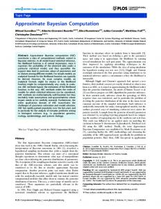
In this section, we present an example to illustrate the methodologies proposed in the previous ones. We considered a CBP starting with Z0 = 1 individual with a geometric distribution with parameter q = 0.4 as offspring distribution and control variables φn (k) following a binomial distribution with parameters ξ(k) and γ = 0.75, where ξ(k) = k + ⌊log(k)⌋, for each k ∈ N and ξ(0) = 0, with ⌊x⌋ denoting the integer part of a number x. Note that the geometric distribution arises naturally as an offspring distribution in the context of branching processes, for example, when embedding the continuous time Markov branching process applied to model data from yeast cells (see Guttorp (1991), p.158), or in other fields as, for example, Physics (e.g. Corral, Garc´ıa-Mill´an, and Font-Clos (2016)). Observe that the control laws combine a deterministic control which is followed by a random control. In particular, these distributions enable to model animal populations with an incorporation of new ones to the population according to the function ξ(·), whereas the binomial distribution may describe the presence of predators, in such a way that γ represents the probability that a progenitor survives and participates in the posterior evolution of the population. Under the above considerations, the offspring distribution and control laws belong to the power series family of distributions. The natural 0 5 10 15 20 25 30 parameter of the geometric distribution as an eleGenerations ment of the power series family of distributions is θ = 1 − q = 0.6. Regarding the offspring mean Figure 1: Temporal evolution of the and variance, one has m = θ(1 − θ)−1 = 1.5 and number of individuals (solid line) σ 2 = θ(1−θ)−2 = 3.75, the control means are ε(k) = and progenitors (dashed line). γξ(k) = 0.75ξ(k), k ∈ N0 , and the asymptotic mean growth rate, defined as τm = limk→∞ ε(k)k −1 m, is τm = γθ(1 − θ)−1 = 1.125. Thus, bearing in mind the value of this threshold parameter, the CBP is supercritical according to the classification of CBPs established in Gonz´alez, Molina, and del Puerto (2005). We simulated the first 30 generations of such a CBP, whose temporal evolution is plotted in Figure 1 (see Table 3 in Subsection 6.1 of the Supplementary material for further details). In this context, the results obtained by using the different ABC algorithms proposed in Section 3 are compared with the output of a “likelihood free” MCMC method, namely, the Gibbs sampler algorithm. In Gonz´alez, Guti´errez, Mart´ınez, Minuesa, and del Puerto (2016), the Gibbs sampler algorithm for the sample made up by the population sizes was implemented in the context on CBPs by considering a non-parametric framework for the offspring distribution and that the control laws belong to the family of power series dis-
12
Individuals Progenitors
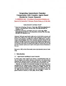
tributions. Without too much difficulty one can also develop and implement the Gibbs sampler for a CBP by assuming a parametric framework for the offspring law and by considering the sample given by the population sizes in each generation and the number of progenitors in the last generation. Since we assumed no information on the plausible values of the offspring and control parameters is available, beta distributions with both parameters equal to 1, i.e. uniform distributions on (0,1), were used as prior distributions for the offspring and control parameters in the ABC methodologies and the Gibbs sampler. We shall start by showing the results for the tolerance-rejection algorithms described in Subsection 3.1. We simulated the first 30 generations of 9 millions of non-extinct CBPs, assuming that it is known that the offspring distribution is a geometric distribution and the control variables are composition of the function ξ(·) (considered known) and variables following binomial distributions with the same probability parameter. For each one of these processes, we computed the sample Ze30 and the summary statistic S(Ze30 ) proposed in (3). As suggested in Beaumont, Zhang, and Balding (2002), we chose as the tolerance level ǫ for both algorithms the quantile qδ of the sample of the distances for the simulated processes, taking δ = 0.025%, that is, the sample quantile of order 2.5 · 10−4 . As a result, the samples obtained by both algorithms have length equal to 2250. Based on these samples, we estimated the posterior density of the parameters θ and γ by means of kernel density estimation using the samples obtained from the tolerance-rejection algorithm without and with the summary statistic. In both cases, we have obtained that the estimates given by the use of ρ1 , ρe and ρH , are very similar. With the aim of presenting the graphs in a clearer way, we only illustrate the results with the metric ρ1 plotted in dashdotted lines in Figures 2 and 3. Numerical results with the other metrics are showed in Table 1 for the parameter θ, and in Table 2 for the parameter γ. It is important to highlight that the estimated posterior densities differ from the density obtained by using the Gibbs sampler algorithm, especially in the case of Algorithm 1, where no reduction of the dimension of the sample was carried out. To improve such estimates, we ran the post-processing algorithms described in Subsection 3.3, the local linear regression Algorithm 3 and the corresponding one with the summary statistic on the associated samples. The resulting samples of these post–processing algorithms are considered to estimate the posterior distributions again. The new estimated posterior densities are plotted in dashed lines in Figures 2 and 3. One can observe that the spread of the new density functions is reduced and the adjustment to the densities given by the Gibbs sampler algorithm is much better than for the tolerance-rejection algorithms; this fact is especially remarkable in the case of the summary statistic in Figures 2 (right) and 3 (right), what evinces the success in using an appropriate summary statistic.
13
30 25
30 25
20 15 5 0
0
5
10
15
Density
20
ABC Rejection ρ1 ABC Regression ρ1 MCMC
10
Density
ABC Rejection ρ1 ABC Regression ρ1 MCMC
0.45
0.50
0.55
0.60
0.65
0.70
0.75
0.80
0.52
0.54
0.56
0.58
0.60
0.62
0.64
0.66
12 8 0
2
4
6
Density
8 6 0
2
4
Density
ABC Rejection ρ1 ABC Regression ρ1 MCMC
10
ABC Rejection ρ1 ABC Regression ρ1 MCMC
10
12
Figure 2: Posterior density of θ estimated by using Gibbs sampler algorithm (solid black line), the tolerance-rejection algorithm (dashdotted lines) and the local linear regression algorithm (dashed lines) for the metric ρ1 . Left: without the summary statistic. Right: with the summary statistic. Vertical lines represent the true value of the parameters.
0.4
0.6
0.8
1.0
0.6
0.7
0.8
0.9
Figure 3: Posterior density of γ estimated by using Gibbs sampler algorithm (solid black line), the tolerance-rejection algorithm (dashdotted lines) and the local linear regression algorithm (dashed lines) for the metric ρ1 . Left: without the summary statistic. Right: with the summary statistic. Vertical lines represent the true value of the parameters.
14
30
30
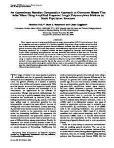
Aiming at improving the estimation of the posterior densities obtained by the previous methods, we also implemented the SMC ABC algorithms described in Subsection 3.2, updating the proposal distribution twice, that is, taking M = 3. In order to obtain samples with length equal to 2250 at the three iterations, we simulated pools of 9 · 104 , 9 · 105 , and 9 · 106 non-extinct CBPs at the corresponding iterations and fixed as the thresholds ǫ1 , ǫ2 and ǫ3 the quantiles of order 0.025, 0.0025, and 0.00025, respectively, of the sample of the distances of the simulated processes. We performed the SMC ABC algorithm without any summary statistic - Figures 4 (left) and 5 (left) - and by reducing the dimension of the data with the summary statistic proposed - Figures 4 (right) and 5 (right) -; in both cases, the estimates of the posterior density based on each sample are plotted in dashdotted lines. As observed for the previous methods, the algorithm without the summary statistic provides a worse estimation than when considering the dimension reduction of the data; note that only in the latter case, the estimated posterior differs slightly from the posterior estimated by the Gibbs sampler. To obtain a more accurate estimation of the posterior density, we ran again post-processing algorithms by using linear regression to the output of the SMC ABC algorithm; the results are represented in Figures 4 and 5 as well and indicate the goodness of the local linear regression algorithms. The joint posterior densities π(θ, γ | Ze30 ) and π(m, γ | Ze30 ) estimated by using the postprocessing correction method on the output of the SMC ABC algorithm with the summary statistic are plotted in Figure 6 for the metric ρ1 .
Density
10
15
20
25 20 15
0
0
5
5
10
Density
SMC ABC ρ1 Regression ρ1 MCMC
25
SMC ABC ρ1 Regression ρ1 MCMC
0.50
0.55
0.60
0.65
0.70
0.54
0.56
0.58
0.60
0.62
0.64
Figure 4: Posterior density of θ estimated by using Gibbs sampler algorithm (solid black line), the SMC ABC algorithm (dashdotted lines) and the local linear regression algorithm (dashed lines) for the metric ρ1 . Left: without the summary statistic. Right: with the summary statistic. Vertical lines represent the true value of the parameters.
15
6
Density
8
10
12
SMC ABC ρ1 Regression ρ1 MCMC
0
2
4
6 0
2
4
Density
8
10
12
SMC ABC ρ1 Regression ρ1 MCMC
0.4
0.5
0.6
0.7
0.8
0.9
1.0
0.65
0.70
0.75
0.80
0.85
Figure 5: Posterior density of γ estimated by using Gibbs sampler algorithm (solid black line), the SMC ABC algorithm (dashdotted lines) and the local linear regression algorithm (dashed lines) for the metric ρ1 . Left: without the summary statistic. Right: with the summary statistic. Vertical lines represent the true value of the parameters.
10
0.80
0.80
50 150
30
250
50
γ
●
60
0.75
400
0.75
γ
350
●
300
40 100
0.58
0.60
20
0.70
0.70
200
0.62
0.64
1.3
1.4
1.5
1.6
1.7
m
θ
Figure 6: Contour plots of the joint posterior densities estimated by the SMC ABC algorithm with the summary statistic and the metric ρ1 followed by the post-processing correction method, together with the true value of the parameters. Left: posterior density of (θ, γ). Right: posterior density of (m, γ) together with the curve γm = 1.125.
16
As we pointed out before, for this particular example we present some summary statistics to evaluate and compare the results obtained by the MCMC methodology and the ABC methods in Table 1 for the parameter θ, and in Table 2 for the parameter γ. First of all, in both cases we provide an estimate for the mean, variance and 95% HPD intervals of the posterior densities based on the samples obtained by each ABC method and by Gibbs sampler. One can observe that, as before, the estimates are improved after using the local-linear regression algorithm on the outputs of the ABC rejection algorithm or the SMC ABC algorithm. In addition, note that there is no significant difference among the results obtained with the different metrics for each method. Next, we present three measures to evaluate the accuracy of the different methodologies: the relative mean square error (RMSE), the integrated squared error (ISE) and the KullbackLeibler divergence between the posterior densities (KL). The RMSE was introduced in Beaumont, Zhang, and Balding (2002) and it enables to compare the mean squared error with the square of the corresponding parameter. The results in the tables indicate that, in both cases, when we do not use the summary statistic and when we use it, it is the SMC ABC algorithm combined with the local-linear regression algorithm the method that best fits the posterior density around the true value of the parameters. We also computed the ISE and the KL for the posterior densities estimated by ABC algorithms and taking the posterior density given by the Gibbs sampler algorithm as the reference posterior density. Again, the SMC ABC algorithm together with the local linear regression algorithm is the algorithm that gives the best fit to the reference posterior density, for both parameters, except in the case of the parameter θ when using the summary statistic; in that case, the ABC rejection algorithm followed by the local linear regression algorithm provides the less values for the ISE and the KL. Moreover, for each ABC method, one can notice that the use of the summary statistic usually reduces the values of the RMSE, ISE and KL. Therefore, in view of this comparison among the different methods, one infers that the SMC ABC algorithm with the summary statistic together with the local-linear regression method provides the best estimate of the true posterior density function. To complete the study of this simulated example, we developed a sensitivity analysis on the choices of the prior distributions. Recall that both the offspring and control parameters are probabilities, and hence, beta distributions as prior distributions for both parameters seem to be reasonable options. Thus, the aforementioned analysis was performed by considering different values for the shape parameters of beta distributions. We summarize the results of this analysis for the Gibbs sampler algorithm and the SMC ABC algorithm with the summary statistic together with the regression using the metric ρ1 in Tables 4 and 5 for the posterior densities π(θ|Ze30 ) and π(γ|Ze30 ), respectively (see Subsection 6.2 of the Supplementary material). We have omitted the results for the remaining algorithms for sake of brevity and only showed the results for the MCMC method and the SMC ABC algorithm with the local-linear regression method since it is the ABC algorithm that provides the best estimate of the posterior densities according to Tables 1 and
17
With the summary statistic
Without any summary statistic
2. The results in Tables 4 and 5 indicate that the estimation of the posterior densities are not sensitive to the choices of the prior distributions. π(θ|Ze30 )
Method
Mean
Variance
95% HPD
RMSE
ISE
KL
MCMC
0.6010
0.0002
[0.5746, 0.6283]
0.0005
·
·
ABC Rejection ρ1
0.5855
0.0028
[0.4976, 0.6928]
0.0083
14.1544
1.1008
ABC Rejection ρe
0.5875
0.0030
[0.4940, 0.7012]
0.0089
13.7924
1.0935
ABC Rejection ρH
0.5867
0.0030
[0.4953, 0.6990]
0.0087
14.1877
1.1221
ABC Regression ρ1
0.5998
0.0004
[0.5580, 0.6414]
0.0012
1.1792
0.0945
ABC Regression ρe
0.6022
0.0006
[0.5540, 0.6485]
0.0015
2.0042
0.1504
ABC Regression ρH
0.6004
0.0005
[0.5564, 0.6435]
0.0013
1.5739
0.1207
SMC ABC ρ1
0.5785
0.0019
[0.5020, 0.6634]
0.0065
13.9647
1.0107
SMC ABC ρe
0.5792
0.0021
[0.5020, 0.6714]
0.0071
14.3270
1.0691
SMC ABC ρH
0.5777
0.0019
[0.5016, 0.6679]
0.0068
14.0251
1.0253
SMC ABC Regression ρ1
0.5935
0.0003
[0.5694, 0.6317]
0.0009
2.7489
0.1350
SMC ABC Regression ρe
0.6040
0.0003
[0.5703, 0.6406]
0.0009
0.8334
0.0584
SMC ABC Regression ρH
0.6004
0.0003
[0.5643, 0.6372]
0.0009
0.5139
0.0449
ABC Rejection ρ1
0.5866
0.0004
[0.5496, 0.6265]
0.0016
7.9818
0.3902
ABC Rejection ρe
0.5876
0.0004
[0.5522, 0.6274]
0.0014
7.2521
0.3486
ABC Rejection ρH
0.5876
0.0004
[0.5522, 0.6274]
0.0014
7.2521
0.3486
ABC Regression ρ1
0.5983
0.0002
[0.5678, 0.6287]
0.0007
0.6802
0.0337
ABC Regression ρe
0.5988
0.0002
[0.5687, 0.6292]
0.0006
0.5594
0.0258
ABC Regression ρH
0.5988
0.0002
[0.5687, 0.6292]
0.0006
0.5596
0.0258
SMC ABC ρ1
0.5922
0.0002
[0.5647, 0.6229]
0.0008
3.8124
0.1813
SMC ABC ρe
0.5920
0.0002
[0.5634, 0.6203]
0.0008
4.0143
0.1911
SMC ABC ρH
0.5922
0.0002
[0.5651, 0.6212]
0.0007
3.8451
0.1811
SMC ABC Regression ρ1
0.5966
0.0002
[0.5665, 0.6212]
0.0005
1.3673
0.0571
SMC ABC Regression ρe
0.5958
0.0002
[0.5687, 0.6216]
0.0005
1.6434
0.0835
SMC ABC Regression ρH
0.5955
0.0002
[0.5700, 0.6221]
0.0005
1.8848
0.0864
Table 1: Summary of the estimates of the posterior density π(θ|Ze30 ) by the different methods. 18
Without any summary statistic With the summary statistic
π(γ|Ze30 )
Method
Mean
Variance
95% HPD
RMSE
ISE
KL
MCMC
0.7531
0.0009
[0.6935, 0.8115]
0.0017
·
·
ABC Rejection ρ1
0.7828
0.0213
[0.4744, 1]
0.0397
6.6761
1.3116
ABC Rejection ρe
0.7717
0.0227
[0.4540, 1]
0.0412
6.6102
1.3100
ABC Rejection ρH
0.7764
0.0224
[0.4580, 1]
0.0410
6.6647
1.3190
ABC Regression ρ1
0.7522
0.0026
[0.6494, 0.8457]
0.0046
0.8155
0.1475
ABC Regression ρe
0.7465
0.0034
[0.6320, 0.8591]
0.0061
1.6037
0.2582
ABC Regression ρH
0.7522
0.0030
[0.6461, 0.8554]
0.0053
1.1930
0.2020
SMC ABC ρ1
0.8010
0.0153
[0.5491, 1]
0.0319
6.2914
1.1647
SMC ABC ρe
0.7959
0.0173
[0.5247, 1]
0.0346
6.5377
1.2406
SMC ABC ρH
0.8009
0.0160
[0.5491, 1]
0.0331
6.4582
1.2071
SMC ABC Regression ρ1
0.7694
0.0016
[0.6793, 0.8314]
0.0035
1.0978
0.1508
SMC ABC Regression ρe
0.7527
0.0020
[0.6668, 0.8421]
0.0036
0.5740
0.1026
SMC ABC Regression ρH
0.7566
0.0021
[0.6670, 0.8475]
0.0038
0.5427
0.1084
ABC Rejection ρ1
0.7629
0.0022
[0.6692, 0.8506]
0.0042
1.3500
0.1877
ABC Rejection ρe
0.7644
0.0022
[0.6714, 0.8533]
0.0043
1.5051
0.2030
ABC Rejection ρH
0.7644
0.0022
[0.6714, 0.8533]
0.0043
1.5051
0.2030
ABC Regression ρ1
0.7633
0.0014
[0.6883, 0.8355]
0.0028
0.7667
0.0918
ABC Regression ρe
0.7626
0.0013
[0.6879, 0.8310]
0.0027
0.7016
0.0800
ABC Regression ρH
0.7626
0.0013
[0.6879, 0.8310]
0.0027
0.7017
0.0800
SMC ABC ρ1
0.7606
0.0012
[0.6936, 0.8301]
0.0023
0.3144
0.0444
SMC ABC ρe
0.7617
0.0012
[0.6945, 0.8270]
0.0023
0.4288
0.0519
SMC ABC ρH
0.7624
0.0012
[0.6963, 0.8257]
0.0023
0.4631
0.0546
SMC ABC Regression ρ1
0.7590
0.0010
[0.7039, 0.8519]
0.0019
0.1746
0.0240
SMC ABC Regression ρe
0.7588
0.0009
[0.6976, 0.8186]
0.0018
0.1884
0.0214
SMC ABC Regression ρH
0.7606
0.0010
[0.7021, 0.8168]
0.0019
0.3130
0.0334
Table 2: Summary of the estimates of the posterior density π(γ|Ze30 ) by the different methods. The ABC methodology relies on having ease of sampling from the model. In our development, this implies the knowledge of the parametric families. An interesting issue
19
is to study the performance of the algorithms when one knows that those distributions can be parametrized with a one-dimensional parameter, but it is unknown the kind of parametric distribution one should use to that end. To evaluate the behaviour of this methodology regarding this problem, apart from the previous example, we simulated two additional CBPs starting with one individual: the first of them has a geometric distribution with parameter θ = 0.918 as the offspring distribution and the control variables φn (k) follow binomial distributions with parameters ξ(k) and γ = 0.1, and in the second CBP, the offspring distribution is a geometric distribution with parameter θ = 0.556 and it has control variables φn (k) following binomial distribution with parameters ξ(k) and γ = 0.9. We proposed two offspring laws (geometric and Poisson distributions) and three control laws (binomial, Poisson and negative binomial distribution) and ran the SMC ABC algorithm with the summary statistic together with the local-linear regression algorithm using the metric ρ1 for the posterior densities π(m|Ze30 ), π(τ |Ze30 ) and π(τm |Ze30 ) in each one of these six situations for the three examples considered. We opted for these three parameters since it is more reasonable to compare the results based on different distributions in terms of the offspring mean, the parameter τ and the asymptotic mean growth rate of the process, which are the stable parameters of the process. As done before, we only present the results for the aforementioned algorithm in Table 6 (see Subsection 6.2 of Supplementary material) for sake of simplicity; we also omitted the results for the Gibbs sampler algorithm since a similar analysis was carried out for the same purpose in Gonz´alez, Guti´errez, Mart´ınez, Minuesa, and del Puerto (2016). The results show that the method for the different models used for simulating usually identify the offspring mean, the parameter τ and the asymptotic mean growth rate relatively well, what also indicates the goodness of our summary statistic. A noteworthy result is the case of considering a Poisson distribution for the control laws. While the algorithm provides a good estimation for the posterior density of the parameter τ , the posterior density for m (and consequently, for τm ) does not seem to fit so well to the one obtained for the second simulated model when assuming a binomial or negative binomial distribution for the control laws. This is related to the magnitude of the parameter θ = 0.918. Indeed, when we used the geometric distribution for simulating the model we also estimated the posterior density of θ, resulting a mean value of 0.9079 and variance of 2.0629 · 10−05 , which seems to be a good estimation of that posterior density. However, the small bias observed in this estimation was enlarged when we estimated m due to the fact that m = θ(1 − θ)−1 . Remark 2. The simulations were performed by the statistical software R (see R Core Team (2017)). For the convergence diagnostics of the Gibbs sampler algorithm we used the coda package (see Plummer, Best, Cowles, and Vines (2006)). Regarding the multivariate normal distribution of algorithm SMC ABC, we made use of the function dmvnorm() of the mvtnorm package for the density function (see Genz, Bretz, Miwa, Mi, Leisch, Scheipl, and Hothorn (2017)) and the function mvrnorm() from the MASS package to draw pairs of numbers of such distributions (see Venables and Ripley (2002)).
20
5
Concluding remarks
Motivated by the interest of making inference on the context of CBPs with random control functions, we have developed ABC methodologies based on the use of an appropriate summary statistic. Thus, this work constitutes a twofold generalization of Gonz´alez, Guti´errez, Mart´ınez, and del Puerto (2013): on the one hand, we considered CBPs with random control functions, and on the other hand, we introduced an appropriate summary statistic to avoid the problem of the dimensionality of the data. To that end, we considered parametric frameworks for the offspring and control distributions and assumed that one can observe all the population sizes and the number of progenitors in the last generation. It is worthwhile to highlight that the knowledge of the number of progenitors in the last generation, φn−1 (Zn−1 ), and its inclusion in the summary statistic, plays an important role when identifying the true parameters of the model and this entails a clear progress with respect to the aforesaid paper. We have proposed several ABC algorithms to sample from the posterior distributions of the offspring and control parameters. We have also approximated the corresponding posterior densities by making use of kernel density estimators. First, we have presented the tolerance-rejection algorithm and proposed a three-dimensional summary statistic in order to reduce the bias of the estimates as a consequence of the large dimension of the data. We also described a SMC ABC algorithm with the suggested summary statistic that has proven to be adequate to draw samples from posterior densities which are closer to the true posterior densities and consequently, it represents an improvement of the tolerance-rejection algorithm. With the aim of refining the sample obtained via each one of those methods, a post-processing based on a local-linear regression is detailed as well. Finally, the accuracy of the ABC procedures have been compared with the output of the Gibbs sampler. We implemented these methodologies by using the statistical software and programming environment R. We developed an extensive analysis of those methods by making use of a simulated CBP. First, we showed a visual comparison of the posterior density estimated by each algorithm and second, a comparison based on summary statistics such as the posterior mean and variance, 95% HPD intervals, RMSE, ISE and KL. The results of this example show that the SMC ABC algorithm with summary statistic together with the local-linear regression post-processing is the preferable method, providing estimates of the posterior densities which are as accurate as the ones obtained with the Gibbs sampler and having the advantage of being computationally simpler. Moreover, a study of the influence of the choice of the prior distributions and the offspring and control distribution considered in the model was carried out, showing that this methodology is not sensible to such choices.
21
Acknowledgements This research has been supported by the Ministerio de Educaci´on, Cultura y Deporte (grant FPU13/03213), the Ministerio de Econom´ıa y Competitividad (grant MTM201570522-P), the Junta de Extremadura (grant IB16099) and the Fondo Europeo de Desarrollo Regional.
6 6.1
Supplementary material Simulated data
The data for the simulated example are provided in Table 3. Recall that for the simulated CBP, which starts with Z0 = 1 individual, the reproduction law is a geometric distribution with parameter q = 0.4, and for each k ∈ N0 , the probability distribution of the control variable φn (k) is a binomial distribution with parameters ξ(k) and γ = 0.75, with ξ(k) = k + ⌊log(k)⌋, for each k ∈ N and ξ(0) = 0.
6.2
Sensitivity analysis
A summary of the sensitivity analysis on the choice of the parameters of the prior distribution is presented in Tables 4 and 5 for the posterior distribution of θ and γ, respectively. The results are provided for the Gibbs sampler algorithm and the SMC ABC algorithm with the summary statistic followed by the post-processing correction method using the metric ρ1 . Finally, in Table 6 we present a summary of the results obtained from the sensitivity analysis on the choice of the parametric families for the offspring and control distributions for three different CBPs. Two families of distributions were considered for the offspring law: geometric and Poisson distribution, and three control laws: binomial, Poisson and negative binomial distribution (denoted by B(ξ(k), ρ), P(ξ(k)λ), and NB(ξ(k), ̺), respectively). For sake of simplicity, the results are only shown for the post-processing method applied on the output of the SMC ABC algorithm with the metric ρ1 and the summary statistic.
22
n 0 1 2 3 4 5 6 7 8 9 10 11 12 13 14 15 16 17 18 19 20 21 22 23 24 25 26 27 28 29 30
Zn φn (Zn ) 1 1 4 3 6 5 4 3 11 10 6 7 9 7 19 13 26 19 14 9 10 9 11 9 9 7 12 8 14 12 15 12 9 5 3 3 6 7 13 13 17 15 23 18 35 32 58 46 75 61 73 51 103 78 107 83 141 100 166 131 216 ·
obs Table 3: Simulated data, Ze30 .
23
Gibbs sampler SMC ABC Regression ρ1
π(θ)
π(γ)
Beta distribution
Beta distribution
Mean
Variance
β(1, 3)
β(1, 3)
0.6023
β(1, 3)
β(0.5, 0.5)
β(1, 3)
π(θ|Ze30 )
95% HPD
RMSE
0.0002
[0.5740, 0.6303]
0.0006
0.5995
0.0002
[0.5721, 0.6273]
0.0005
β(3, 1)
0.5997
0.0002
[0.5710, 0.6280]
0.0006
β(0.5, 0.5)
β(1, 3)
0.6027
0.0002
[0.5764, 0.6302]
0.0006
β(0.5, 0.5)
β(0.5, 0.5)
0.6009
0.0002
[0.5731, 0.6288]
0.0006
β(0.5, 0.5)
β(3, 1)
0.6003
0.0002
[0.5737, 0.6283]
0.0005
β(3, 1)
β(1, 3)
0.6040
0.0002
[0.5770, 0.6311]
0.0006
β(3, 1)
β(0.5, 0.5)
0.6014
0.0002
[0.5743, 0.6281]
0.0005
β(3, 1)
β(3, 1)
0.6013
0.0002
[0.5732, 0.6308]
0.0006
β(1, 3)
β(1, 3)
0.5961
0.0002
[0.5704, 0.6225]
0.0005
β(1, 3)
β(0.5, 0.5)
0.5953
0.0002
[0.5708, 0.6209]
0.0005
β(1, 3)
β(3, 1)
0.5956
0.0002
[0.5706, 0.6211]
0.0005
β(0.5, 0.5)
β(1, 3)
0.5982
0.0002
[0.5726, 0.6255]
0.0005
β(0.5, 0.5)
β(0.5, 0.5)
0.5966
0.0002
[0.5718, 0.6221]
0.0005
β(0.5, 0.5)
β(3, 1)
0.5961
0.0002
[0.5719, 0.6234]
0.0005
β(3, 1)
β(1, 3)
0.5982
0.0002
[0.5734, 0.6250]
0.0005
β(3, 1)
β(0.5, 0.5)
0.5958
0.0002
[0.5712, 0.6219]
0.0005
β(3, 1)
β(3, 1)
0.5961
0.0002
[0.5714, 0.6214]
0.0005
Table 4: Summary of the sensitivity analysis on the choice of the prior distribution for the posterior density π(θ|Ze30 ).
24
Gibbs sampler SMC ABC Regression ρ1
π(θ)
π(γ)
Beta distribution
Beta distribution
Mean
Variance
β(1, 3)
β(1, 3)
0.7464
β(1, 3)
β(0.5, 0.5)
β(1, 3)
π(γ|Ze30 )
95% HPD
RMSE
0.0010
[0.6831, 0.8077]
0.0018
0.7561
0.0009
[0.6939, 0.8144]
0.0017
β(3, 1)
0.7576
0.0009
[0.6985, 0.8121]
0.0017
β(0.5, 0.5)
β(1, 3)
0.7460
0.0009
[0.6849, 0.8035]
0.0017
β(0.5, 0.5)
β(0.5, 0.5)
0.7533
0.0010
[0.6874, 0.8109]
0.0018
β(0.5, 0.5)
β(3, 1)
0.7573
0.0009
[0.6974, 0.8151]
0.0017
β(3, 1)
β(1, 3)
0.7444
0.0010
[0.6820, 0.8051]
0.0018
β(3, 1)
β(0.5, 0.5)
0.7534
0.0009
[0.6933, 0.8120]
0.0017
β(3, 1)
β(3, 1)
0.7544
0.0009
[0.6935, 0.8137]
0.0017
β(1, 3)
β(1, 3)
0.7581
0.0010
[0.6934, 0.8163]
0.0019
β(1, 3)
β(0.5, 0.5)
0.7604
0.0009
[0.6951, 0.8164]
0.0019
β(1, 3)
β(3, 1)
0.7617
0.0009
[0.6989, 0.8164]
0.0019
β(0.5, 0.5)
β(1, 3)
0.7496
0.0011
[0.6845, 0.8092]
0.0019
β(0.5, 0.5)
β(0.5, 0.5)
0.7607
0.0010
[0.6951, 0.8183]
0.0020
β(0.5, 0.5)
β(3, 1)
0.7617
0.0010
[0.6955, 0.8190]
0.0020
β(3, 1)
β(1, 3)
0.7535
0.0010
[0.6872, 0.8099]
0.0018
β(3, 1)
β(0.5, 0.5)
0.7602
0.0009
[0.6974, 0.8165]
0.0018
β(3, 1)
β(3, 1)
0.7591
0.0009
[0.6958, 0.8126]
0.0017
Table 5: Summary of the sensitivity analysis on the choice of the prior distribution for the posterior density π(γ|Ze30 ).
25
Geometric offspring distribution Model
Parameter
φn (k) ∼ B(ξ(k), 0.75)
Xni ∼ G(0.6),
m = 1.5
τ = 0.75
τm = 1.125
φn (k) ∼ B(ξ(k), 0.1)
Xni ∼ G(0.918),
m = 11.25
τ = 0.1
τm = 1.125
φn (k) ∼ B(ξ(k), 0.9)
Xni ∼ G(0.556),
m = 1.25
τ = 0.9
τm = 1.125
Poisson offspring distribution
Summary
B(ξ(k), ρ)
P(ξ(k)λ)
N B(ξ(k), ̺)
B(ξ(k), ρ)
P(ξ(k)λ)
N B(ξ(k), ̺)
Mean
1.4766
1.4595
1.5224
1.4999
1.5235
1.5864
Variance
0.0066
0.0178
0.0323
0.0046
0.0141
0.0308
RMSE
0.0032
0.0087
0.0146
0.0021
0.0065
0.0170
Mean
0.7588
0.7628
0.7385
0.7564
0.7451
0.7149
Variance
0.0009
0.0047
0.0073
0.0010
0.0039
0.0071
RMSE
0.0018
0.0086
0.0133
0.0018
0.0070
0.0147
Mean
1.1190
1.1058
1.1109
1.1330
1.1288
1.1209
Variance
0.0024
0.0033
0.0043
0.0012
0.0023
0.0032
RMSE
0.0019
0.0029
0.0035
0.0010
0.0018
0.0026
Mean
11.1501
9.8923
11.0885
11.0387
9.1979
10.9420
Variance
0.3058
0.2947
0.3709
0.2482
0.0441
0.3230
RMSE
0.0025
0.0159
0.0030
0.0022
0.0322
0.0031
Mean
0.0979
0.0992
0.0984
0.0989
0.1039
0.0997
Variance
0.00002
0.0001
0.00003
0.00002
0.00004
0.00003
RMSE
0.0029
0.0054
0.0032
0.0022
0.0055
0.0026
Mean
1.0890
0.9784
1.0884
1.0900
0.9548
1.0887
Variance
0.0007
0.0017
0.0007
0.0003
0.0017
0.0004
RMSE
0.0013
0.0172
0.0014
0.0010
0.0230
0.0011
Mean
1.2555
1.2516
1.2562
1.2578
1.2573
1.2630
Variance
0.0006
0.0022
0.0033
0.0004
0.0018
0.0032
RMSE
0.0004
0.0014
0.0021
0.0002
0.0012
0.0021
Mean
0.9096
0.9133
0.9090
0.9094
0.9107
0.9059
Variance
0.0001
0.0011
0.0017
0.0001
0.0010
0.0018
RMSE
0.0002
0.0015
0.0021
0.0002
0.0013
0.0022
Mean
1.1419
1.1419
1.1399
1.1437
1.1439
1.1421
Variance
0.0004
0.0006
0.0007
0.0002
0.0004
0.0006
RMSE
0.0005
0.0007
0.0007
0.0004
0.0005
0.0006
Table 6: Summary of the sensitivity analysis on the choice of the offspring and control distributions in the SMC ABC algorithm with the summary statistic and the post-processing method. For the reproduction law a geometric distribution and a Poisson distribution were fitted, while for the control laws a binomial distribution, a Poisson distribution and a negative binomial distribution were considered.
26
References M. A. Beaumont, W. Zhang, and D. J. Balding. Approximate Bayesian Computation in population genetics. Genetic, 162(4):2025–2035, 2002. M. A. Beaumont, J. M. Cornuet, J. M. Marin, and C. P. Robert. Adaptive Approximate Bayesian Computation. Biometrika, 96(4):983–990, 2009. N. Becker. On parametric estimation for mortal branching processes. Biometrika, 61(3): 393–399, 1974. A. Corral, R. Garc´ıa-Mill´an, and F. Font-Clos. Exact derivation of a finite-size scaling law and corrections to scaling in the geometric Galton-Watson process. PLoS ONE, 11 (9):1–17, 2016. A. Genz, F. Bretz, T. Miwa, X. Mi, F. Leisch, F. Scheipl, and T. Hothorn. mvtnorm: Multivariate Normal and t Distributions, 2017. URL https://CRAN.R-project.org/package=mvtnorm. R package version 1.0-6. M. Gonz´alez, M. Molina, and I. del Puerto. Asymptotic behaviour of the critical controlled branching processes with random control functions. Journal of Applied Probability, 42 (2):463–477, 2005. M. Gonz´alez, C. Guti´errez, R. Mart´ınez, and I. del Puerto. Bayesian inference for controlled branching processes through MCMC and ABC methodologies. Revista de la Real Academia de Ciencias Exactas, F´ısicas y Naturales. Serie A. Matem´aticas, 107 (2):459–473, 2013. M. Gonz´alez, C. Guti´errez, R. Mart´ınez, C. Minuesa, and I. del Puerto. Bayesian analysis for controlled branching processes. In I. del Puerto, M. Gonz´alez, C. Guti´errez, R. Mart´ınez, C. Minuesa, M. Molina, M. Mota, and A. Ramos, editors, Branching Processes and Their Applications, volume 219 of Lecture Notes in Statistics, pages 185–205. Springer, 2016. M. Gonz´alez, C. Minuesa, and I. del Puerto. Maximum likelihood estimation and Expectation-Maximization algorithm for controlled branching processes. Computational Statistics and Data Analysis, 93:209–227, 2016. M. Gonz´alez, C. Minuesa, and I. del Puerto. Minimum disparity estimation controlled branching processes. Electronic Journal of Statistics, 11(1):295–325, 2017. M. Gonz´alez, I. del Puerto, and G. P. Yanev. Controlled Branching Processes. ISTE Ltd and John Wiley and Sons, Inc., 2018.
27
P. Guttorp. Statistical inference for branching processes. John Wiley and Sons, Inc., 1991. P. Guttorp and M. D. Perlman. Predicting extinction or explosion in a Galton-Watson branching process with power series offspring distribution. Technical Report 626, Department of Statistics, University of Washington, 2014. P. Holgate and K. H. Lakhani. Effect of offspring distribution on population survival. Bulletin of Mathematical Biophysics, 29(4):831–839, 1967. J. Lintusaari, M. U. Gutmann, R. Dutta, S. Kaski, and J. Corander. Fundamentals and recent developments in Approximate Bayesian Computation. Systematic Biology, 66 (1):e66–e68, 2017. R. Mart´ınez, M. Mota, and I. del Puerto. On asymptotic posterior normality for controlled branching processes. Statistics, 43(4):367–378, 2009. T. McKinley, A. R. Cook, and R. Deardon. Inference in epidemic models without likelihoods. The International Journal of Biostatistics, 5(1):Article 24, 2009. J. Owen, D. J. Wilkinson, and C. S. Gillespie. Likelihood free inference for Markov processes: a comparison. Statistical Applications in Genetics and Molecular Biology, 14(2):189–209, 2015. M. Plummer, N. Best, K. Cowles, and K. Vines. CODA: Convergence diagnosis and output analysis for MCMC. R News, 6(1):7–11, 2006. D. Prangle. Adapting the ABC distance function. Bayesian Analysis, 12(1):289–309, 2017. R Core Team. R: A language and environment for statistical computing. R Foundation for Statistical Computing, Vienna, Austria, 2017. URL http://www.R-project.org/. C. P. Robert. Approximate Bayesian Computation: A survey on recent results. In R. Cools and D. Nuyens, editors, Monte Carlo and Quasi-Monte Carlo Methods, volume 163 of Springer Proceedings in Mathematics & Statistics. Springer International Publishing, 2016. D. B. Rubin. Bayesianly justifiable and relevant frecuency calculations for the applied statistician. The Annals of Statistics, 12(4):1151–1172, 1984. B. A. Sevast’yanov and A. M. Zubkov. Controlled branching processes. Theory of Probability and its Applications, 19(1):14–24, 1974. S. Tavar´e, D. J. Balding, R. C. Griffith, and P. Donnelly. Inferring coalescence times from DNA sequence data. Genetics, 145(2):505–518, 1997.
28
W. N. Venables and B. D. Ripley. Modern Applied Statistics with S. Springer, New York, fourth edition, 2002. N. M. Yanev. Conditions for degeneracy of φ-branching processes with random φ. Theory of Probability and its Applications, 20:421–428, 1975.
29