Random Coefficient Models for Time-Series–Cross ... - Semantic Scholar

Random Coefficient Models for Time-Series–Cross-Section Data: The 2001 Version1 Nathaniel Beck2

Jonathan N. Katz3

Prepared for delivery at the 2001 Annual Meeting of the Society for Political Methodology, Emory University. Draft of July 17, 2001

1 We

are grateful to Larry Bartels for always reminding us that our judgment may outperform the data. We thank Geoffrey Garrett for allowing us to use his data. 2 Department of Political Science; University of California, San Diego; La Jolla, CA 92093; [email protected] 3 Division of the Humanities and Social Sciences; California Institute of Technology; Pasadena, CA 91125; [email protected]

Abstract This paper considers random coefficient models (RCMs) for time-series–cross-section data. These models allow for unit to unit variation in the model parameters. After laying out the various models, we assess several issues in specifying RCMs. We then consider the finite sample properties of some standard RCM estimators, and show that the most common one, associated with Hsaio, has very poor properties. These analyses also show that a somewhat awkward combination of estimators based on Swamy’s work performs reasonably well; this awkward estimator and a Bayes estimator with an uninformative prior (due to Smith) seem to perform best. But we also see that estimators which assume full pooling perform well unless there is a large degree of unit to unit parameter heterogeneity. We also argue that the various data driven methods (whether classical or empirical Bayes or Bayes with gentle priors) tends to lead to much more heterogeneity than most political scientists would like. We speculate that fully Bayesian models, with a variety of informative priors, may be the best way to approach RCMs.

1

RCM’s and TSCS Data

We have been examining the estimation of time-series–cross-section (TSCS) models for a long time. While we initially began by examining the properties of various TSCS estimators, our recent work has become much more involved with issues of specifying TSCS models. One critical specification issue is whether to assume that all units are completely homogeneous, that is, are they governed by the same specification and the same set of parameters. Most TSCS analysts seem to assume that the assumption of full pooling is reasonable (that is, they use such a model and seldom offer a test). There are, of course, alternatives to the full pooling assumption. Many analysts allow for unit specific intercepts, that is, fixed effects. But there are relatively few attempts to go beyond this limited heterogeneity. Obviously we must assume enough homogeneity to allow for estimation; if every observation is unique, we can do no science. But it is not necessary to assume that the only alternative to complete uniqueness is complete pooling (or its close cousin, pooling other than in the unit specific intercepts). At first glance, the commitment to homogeneity is a bit odd, since a model which imposes less heterogeneity, the random coefficients model (RCM), is well known, and has been well known for a quarter of a century. One cannot even blame software packages for the lack of use of RCMs, since the RCM is implemented in very common packages in use by political scientists (Stata, Splus, LIMDEP). The other normal prerequisite for political science use, a Workshop piece in the AJPS, has also been fulfilled (Western, 1998). Should TSCS analysts routinely entertain the RCM? Does it work well for the kinds of data typically seen in political science? In this paper we continue the investigation of this question. We begin by noting that the issue of whether to pool or not, or, more accurately, how much to pool, confronts every researcher. In an important, if uncited1 piece, Bartels (1996) argues that we are always in the position of deciding how much we should pool some observations with others, and we always have a choice ranging from complete pooling to assuming that the data have nothing to do with each other. He notes that, in general, political scientists seem to assume that either data completely pool or that some data is completely irrelevant, ignoring the in between position. The solution that Bartels proposes is that one should estimate a model allowing for varying degrees of pooling and then make a scientific decision after examining the locus of all such estimates. The procedure involves much judgment, since Bartels works in a purely cross-sectional context; in that context, the data alone can never determine the appropriate degree of pooling. The situation is happier for the TSCS analyst, since we can assume complete homogeneity within units, and thus limit ourselves to models that imply heterogeneity between units. It is this world we examine here. Western has described the RCM in a Bayesian context. 2 The citation fate of his paper is no happier than that of Bartels.3 We thus must ask, if RCMs 1

The SSCI has five citations to this article, three by qualitative researchers, and, as far as we can tell, no actual empirical applications. 2 Western’s setup is the same as the Bayesian setup first described by Smith (1973). Smith did not have the computational power in 1953 to produce full Bayesian posteriors, and was limited to estimation of the mode of that distribution given a vague prior. 3 Western also has five cites, one by him, two by us, one by his sometime coauthor Simon Jackman and

1

are so good, why does no one seem to use them? The next section of the paper lays out the notation and some mathematics of the RCM and various estimators; Section 3 provides some discussion of the RCM approach; Section 4 provides Monte Carlo evidence on specific estimators. Section 5 looks at one application and Section 6 concludes.

2

Preliminaries

We assume standard TSCS data with a continuous dependent variable.4 freely allow one of the independent variables to be a lagged dependent variable and assume that the errors are temporally independent. The fully pooled model is thus: yi,t = xi,t β + εi,t ; i = 1, . . . , N ; t = 1, . . . , T

(1)

ind

where β is a K-vector of parameters and εi,t ∼ N (0, σ 2 ) (and by assumption is iid). This model can be estimated by some variant of OLS. The less pooled model has yi,t = xi,t βi + εi,t ; i = 1, . . . , N ; t = 1, . . . , T

(2)

We could allow each unit’s βi to be completely unrelated to every unit’s parameters, and thus have the fully unpooled model, which would be estimated by unit by unit OLS. Alternatively, we could estimate the βi by some other method which would allow the estimates of different units to “borrow strength” from each other.5 We can test H0 :Eq 1 against the alternative Eq 2 (completely disparate or unpooled βi ) by a standard F -test using the SSEs from the OLS estimations of both Eq 1 and 2. Typical procedure would then be to go with the pooled model if the F -ratio is small and with the fully unpooled (unit by unit OLS) model if it is large, with small and large being judged relative to 95% critical values of the F -distribution. Note that this procedure yields a “pre-test” estimator, that is, estimate β i by the pooled OLS estimator if the F -ratio is under a critical value and by the fully unpooled OLS estimator if the F -ratio is above this critical value. As with any pre-test estimator, we can improve on matters by finding a “shrinkage” estimator that more smoothly combines the two estimators. one by a former student of one of us. None of these cites seem to have an application of Western’s proposed method. 4 This is to distinguish TSCS data from panel data. In particular, we have fixed, not sampled, units, and all asymptotics are in T , not N ; T is large enough to do some time-series analysis on the data. The distinction between TSCS and panel data is discussed more fully in Beck (2001). Thus nothing said in this paper bears on the suitability of the RCM for panel data; for such data, the RCM is usually known as the hierarchical model (Bryk and Raudenbush, 1992) or the multilevel model (Snijders and Bosker, 1999). That these models are useful for panel data tells us little about their usefulness for TSCS data. 5 In this notation, it looks like all the parameters must be allowed to vary from unit to unit. It is of course possible to force some subset of the β to be fully pooled while allowing for heterogeneity in another subset. This causes no problems and is usually a good thing to do. But for notational simplicity we ignore this at no cost.

2

These pay some attention to the fully pooled estimator if we just barely reject pooling and some attention to the unpooled estimator if we marginally fail to reject the pooled estimator (James and Stein, 1961; Judge and Bock, 1978; Judge, Griffiths, Hill, L¨ utkepohl and Lee, 1985; Maddala and Hu, 1996). Western works in a Bayesian manner, assuming that βi are draws from a normal, so that βi ∼ N (β, Γ)

(3)

where Γ is another parameter to be estimated; it indicates the degree the homogeneity of the unit parameters (Γ = 0 indicates perfect homogeneity).6 To estimate the model he puts a very gentle prior on the various parameters and hyperparameters (β, Γ and σ 2 ).7 As noted, Western uses Bayesian Markov Chain Monte Carlo methods to estimate his model. The methods used are Bayesian, His prior, however, is not based on non-sample information, but rather is a “gentle” prior which is designed to allow the posterior to reflect the data as much as possible, and hence for the prior as little effect on the estimation as possible. But once we accept that the prior should have as little impact if any impact on estimation, it becomes sensible to look at classical methods to estimate the RCM, and choice between these rests on such non-social science issues as convenience, computational costs and the like. The classical estimators of the RCM model, that is, either a full maximum likelihood (ML)8 or a GLS estimate,9 all are different ways of combining estimates of the individual βi , and are all, more or less similar to empirical Bayes methods. Unlike the fully Bayesian method, empirical Bayes methods allow the data to “choose” a prior, that is, the heterogeneity in the βi is estimated from the data (that is, the heterogeneity in the estimated βˆi ), and from then on Bayesian formulae are used. These estimators can all be seen as variants 6

This is the standard setup. Some assume that the βi are not draws from a K-variate normal, but rather K independent draws from univariate normals. This specialization seems sensible, since it cuts the number 2 of variance-covariance parameters to be estimated from approximately K2 to K. We return to this issue below. 7 While it is not our intention to either explicate or critique Western, there are a few features of his model that are of interest but are orthogonal to our interest. In particular, he sensibly assumes that the β i are functions of unit covariates, so that he has βi = β + zi α + νi rather than the form we use which does not have the zi α term. Note that this term just adds (deterministic) interactive terms to the model, which are the elements of zi multiplied by xi,t . While Western’s move here is sensible, it is completely orthogonal to the issues discussed here, and so use the simpler form for the random coefficients. Western’s particular specification here is odd, since he interacts all the xi,t with his one zi whereas the theory he is working with calls for the interaction of only one of the independent variables with his z i . For this and various other reasons, when we do our own empirical work we do not begin with Western’s model or results. 8 This is due to Pinheiro and Bates (2000), though the Smith (1973) iterated Bayesian estimator with an uninformative prior is also ML. 9 Econometricians learn of these models from Swamy (1971) though many know this work through Hsaio (1986). When we discuss specific GLS implementations, we discuss the most common method, which Swamy proposed and Hsaio argued for. We call this “Hsaio.” It is this method that is implemented in standard packages such as Stata or LIMDEP. Note that the same model and estimation technique was developed by the statisticians Hildreth and Houck (1968) prior to the work of Swamy. Thus Stata calls names its GLS RCM estimator for Hildreth and Houck. But the implementation is identical to the GLS implementation we call Hsaio.

3

of “shrinkage” estimators, where the individually estimated βˆi are “shrunk” towards some overall estimate of the mean β. In empirical Bayes methods, the amount of shrinkage is a function of the diversity of the individually estimated βi . Since the estimators do vary, and we wish to compare their performance in our Monte Carlo experiments, we briefly lay out our notation and the various estimators now.

Basic Model and notation Formally the model we are considering is: yi,t = xi,t βi + εi,t βi ∼ N (β, Γ) E[βi − β|xi,t ] = 0 E[εi,t |xi,t ] = 0 ( σi2 if i = j E(εi,t εj,t ) = 0 if i 6= j

(4) .

When we consider ML estimates we will further assume: ind

εi,t ∼ N (0, σi2 ). Note that we could allow the errors to have a more complicated error structure, but this would cloud the central issues. In deriving some results it will be useful to define νi = βi − β. Clearly νi ∼ N (0, Γ). We can re-write the model for the yi,t ’s by substituting as: yi,t = xi,t β + (εi,t + xi,t νi ) yi,t = xi,t β + wi,t .

(5)

with wi,t as our new composite error term. The first part of wi,t is the standard stochastic part of a regression model. The second term is the error associated with how far a particular unit’s βi is from the overall mean β. It will also be convenient to stack the observations by unit instead of considering individual observations. Define         wi,1 εi,1 xi,1 yi,1  wi,2   εi,2   xi,2   yi,2           .   .   .   .  .        wi =  εi =   xi =  yi =     . . . .          .   .   .   .  wi,T εi,T xi,T yi,T 4

If it were the case that wi were suitably well behaved, and, in particular, that E[wi |xi ] = 0, then we could estimate Eq 5 by OLS, which would give us a consistent, although possibly not efficient estimate of β. In fact, we have already made enough assumptions to ensure this. To see this note: E[wi |xi ] = E[εi + xi vi |xi ] = E[εi |xi ] + E[xi vi |xi ] = 0 + xi E[vi |xi ] = 0. The last step is true because we have assumed in the basic setup that βi are mean independent of the xi,t . Therefore, there cannot be a systematic relationship between the unit’s average xi,t and βi . This assumption would fail if units with high values of some regressors also had larger βi . Consider, for example, a comparative model of annual government spending as a function of revenue among other things. It might be the case that governments that are better at raising funds are also more likely to have higher spending — i.e., have a large β i . We thus have our first candidate RCM model: pooled OLS. With pooled OLS we estimate Eq 5 by standard OLS. Our estimate of the individual βi ’s would just be this overall estimate, ˆ That is we are borrowing a lot of strength across units. This model is perhaps the β. most common in the literature. In general, because the estimate in pooled OLS on N × T observations, it will have small sampling variance. As we will see in the simulations below, this small sampling variance makes the pooled OLS estimator perform better than one might expect, even when the assumption of pooling does not hold. We should note, however, our OLS estimates would not be efficient for the overall mean because it is not using the full structure of our model. This can be seen by examining the covariance matrix of the pooled OLS estimate defined by Eq 5: E[wi wi0 ] = E[(εi + xi vi )(εi + xi vi )0 ] = σi2 IT + xi Γx0i = Πi . So for the full sample (stacking observations) the  Π1 0 0  0 Π2 0  Ω= ..  . 0 0 0 = I ⊗ Πi

covariance matrix of OLS estimate of is  ... 0 ... 0   (6)   . . . ΠN (7)

Where ⊗ is the Kronecker product. If we knew Γ, as well as σi2 , we would know Πi and therefore Ω. Estimation would be relatively straightforward generalized least squares (GLS). We will explore this more below. At the other extreme from complete pooling would be to run OLS on each unit. We will refer to this estimate at unit by unit OLS and denote the estimate from the i’th unit by 5

bi . Clearly, this estimate borrows the least strength from other units, and will be consistent even if there is some correlation structure between βi and xi . Asymptotically (as T → ∞) this would be the preferred estimator because we can recover βi regardless of the relationship between units (which is only indirectly of interest in practice). However, in finite samples, this estimator may have very large sampling variance. The remaining estimators we will consider can be thought of as various shrinkage estimators that estimate the βi as a weighted average between the pooled (although the GLS and Bayesian estimators use slightly different choice of the pooled estimate, normally to gain some efficiency) and the unit by unit estimates. They essentially differ in how they determine this weight, that is they shrink the unit by unit estimate back towards the overall mean.

Stein-Rule Perhaps the classical approach to shrinking are the Stein-rule estimators. The complete justification for such estimators is beyond the scope of this paper. As was mentioned before, they were designed to be smooth versions of pre-test estimators (which have very complicated sampling distributions) based on the F test for parameter homogeneity. Accordingly, the weighting between the pooled and unpooled estimators is a function of this test statistic. Formally the Stein-rule estimator for unit level parameters is c c βbi = βˆ + (1 − )bi F F

where βˆ and bi are defined above, F is the statistic for testing the null hypothesis of equality of the βi and c is a constant. Judge and Bock (1978:190–195) suggest that the optimal value for this constant is: (N − 1)k − 2 c= , (8) NT − Nk + 2 where k is the number of regressors.

Generalized Least Squares An alternative shrinkage estimators can be considered in the generalized least squares framework. Recall that the estimate of the overall mean from the pooled OLS was inefficient because it does not use all of the information in the structure of the model. A GLS estimate of β would be: [X0 Ω−1 X]−1 XΩ−1 y Where X = [x1 , x2 , . . . , xN ]0 and y = [y1 , y2 , . . . , yN ]0 . In general, we will not know Γ but will have to estimate it. We will turn to how to estimate it shortly, but for now assume we b We can then construct the feasible generalized have some consistent estimate of Γ, say Γ. least square estimate (FGLS) as follows: b −1 X]−1 XΩ b −1 y β˜ = [X0 Ω 6

(9)

where b = IN ⊗ Π bi Ω

b 0 ). = IN ⊗ (ˆ σi2 IT + xi Γx i

There is an alternative formulation of β˜ as a weighted function of the unit by unit OLS estimates (bi ) which gives us a bit more insight into the GLS estimators. Clearly bi is consistent for βi (and β) by the same assumptions and argument we used to show that OLS using the observations from all units was consistent for the estimate of the overall mean β. Given standard results we can show: Var(bi ) = (x0i xi )−1 x0i Πi (xi (x0i xi )−1 = Vi + Γ, where Vi = σi2 (x0i xi )−1 . Then the GLS estimator given in ( 9) can be written as: β˜ =

N X

(10)

Wi b i

i=1

where Wi =

(

N X

[Γ + Vi ]−1

i=1

)−1

[Γ + Vi ]−1

The GLS estimate, then, is a weighted average of the unit by unit OLS estimates. The weights are such that units that have smaller variance of their estimates, perhaps because they have a larger T or just fit better, are given more weight. ˜ Given Eq 10 and It will also be useful to have an explicit formula for the variance of β. the fact that the bi are independent, the variance is straight forward to derive. ˜ = Var(β) =

N X

i=1 N X

Wi Var(bi )Wi0 (11) Wi [Vi + Γ]Wi0 .

i=1

We can now turn to the estimations of the parameters of interest, βi . The best linear unbiased predictor of βi that comes from the GLS framework is: b −1 ]−1 [Γ−1 β˜ + V b −1 bi ] βbi = [Γ−1 + V = Ai β˜ + [Ik − Ai ]bi

(12)

b −1 ]−1 Γ. That is, the estimate is a weighted average between the pooled where Ai = [Γ−1 + V i and unit by units. The weights are given by the relative precision of our two estimates. 7

We can justify βbi is two ways. From the classical perspective, it minimizes mean squared error given the setup in Eq 4. It is in that sense it is “best”. However, it can also be justified for the Bayesian perspective. If we were interested in estimating the βi and we had a prior of the form, βi ∼ N (β, Γ), this would be our posterior mode estimate. Further, if we are going to estimate β and Γ from observed data (as we will below), we could call this an empirical Bayesian estimate. Depending on how we estimate Γ, we will get different RCM estimators. We now turn to these. It will be useful to define Var(βbi ) in order to do statistical testing. In general, since βbi is estimated by a linear combination we can use standard results to show: ˜ 0 + [Ik − Ai ] Var(bi )[Ik − Ai ]0 + Var(βbi ) = Ai Var(β)A i ˜ bi )A0 + Ai Cov(β, ˜ bi )[Ik − Ai ]0 . [Ik − Ai ] Cov(β,

(13)

i

˜ bi ) = Wi Var(bi ). This his true because the This can be simplified by noting that Cov(β, bi ’s are independent; the only term in the sum that makes up β˜ that has positive covariance with a particular bi is Wi bi . The obstacle for GLS is that we do not know either Γ or Vi , hence we can not use Eq 10 to estimate the overall mean parameter or Eq 12 to estimate βi . However, as is often true with GLS models we can use a two-step procedure. We first consider an estimator originally suggested by Swamy (1971) to estimate Γ and Vi . In the first step we use some consistent, but inefficient, estimator to estimate β and the βi ’s. We then use these preliminary estimates to estimate the variance parameters. In this case, we run OLS unit by unit to estimate b i . We then estimate Vˆi by its usual estimate: Vˆi = s2i (x0i xi )−1 e0 ei s2i = i , T −k where ei are standard OLS residuals and k is the number of regressors. The question is how to estimate Γ? If we could directly observe β1 , . . . , βN , we could use the N draws to construct an estimate of the covariance matrix in the usual fashion: Ã N ! X 1 0 e= Γ βi βi − N ββ 0 , N − 1 i=1

where β¯i is the mean of the N observed βi . We note that any such estimate of Γ will improve e will converge in probability to Γ using standard assumptions. as N get large. Formally Γ While this is important to panel analysts, who can allow for asymptotics in N , it is of cold comfort to TSCS analysts who must work with fixed, and typically not very large, N s. This issue is muted a bit if we take an empirical Bayesian perspective. The point of the empirical Bayes approach is not to estimate Γ, per se, but to use it in forming of a prior to improve our estimates of βi . Clearly there is information in the data about Γ even when N is fixed. Again the problem is we do not observe βi ; we have, instead, only a noisy estimates of e this the bi . So while we might consider just substituting bi for βi in the definition of Γ, 8

would lead us to over estimate the amount of variation in βi since much of the variation in the bi s is caused not by “real” parameter variability but purely by sampling error. In finite samples we would expect the bi ’s to differ. We can correct for this sampling variability by ˆ Swamy suggested that a plausible estimator of Γ is noting that the Var bi = Vi + β. ! Ã N N X 1 1 Xb 0 0 b bi bi − N bb − Vi , (14) Γ= N − 1 i=1 N i=1

where b is the mean of the bi ’s. Thus the Swamy estimator plugs in the estimate for Γ into the formula for βbi . b (defined by Eq 14) There is, however, a problem with this estimator: in finite samples Γ need not be positive definite, a necessary requirement for it to be a well defined covariance b may not be positive definite because we are subtracting off the mean Vbi , which matrix. Γ can be large in finite samples. Recall that Vbi is the estimated sampling variability of the OLS estimate for unit i. If, for example, T is small, as it usually is in practice, we would expect Vbi to be large and to dwarf the effect of the parameter heterogeneity estimated by the first term. The question is how to insure that our estimate of Γ is positive definite? Hsaio’s (1986, 131–4) suggestion, building on Swamy, is to drop the second term in the estimate of Γ, which seems to be the accepted practice.10 Thus we get the Hsaio estimator by plugging this estimate of Γ into Eq 12. The rationale for this is asymptotic. The first term of Eq 14 is of O(1) whereas the second term is O( N1T ). In words the first term does not vanish as either N or T gets large since it is the estimate of the “true” parameter variability. The second term is sampling variability, so as T get large our estimate bi converge to their true values βi , so the second term in Eq 14 vanishes asymptotically in T . Note that this fix is not correct in finite samples as it will tend to overestimate Γ. The interesting question is how badly does this affect the estimate of Γ and does this cause any problems in the estimates of βi ? Since these are problems in finite samples we will have to assess the claims using Monte Carlo simulations in Section 4. As alluded to above, we might be concerned that Hsaio estimate of Γ will be too large. b the less we shrink. We might want to err If we look at the formula for βbi , the larger is Γ, the other way. So another possible estimator which we will refer to as BKK (for Beck-Katz kludge) is ! " Ã N # N X X 1 1 0 b = max 0, Γ bi b0i − N bb − Vbi , N − 1 i=1 N i=1 That is, we use the Swamy estimator that corrects for sampling when it is positive definite; b to zero (which means we are using the fully pooled OLS estimate of βi ). This if not we set Γ will have a complicated sampling distribution, but may work well in practice since it errs towards greater pooling. We will explore the finite sample properties of this estimator in Section 4. 10

This is how the RCM estimator is coded in both Stata and LIMDEP.

9

Bayesian and Maximum Likelihood Estimation An alternative approach to two step FGLS estimate is a direct maximization of the likelihood. This can form the basis of either classical (i.e., maximum likelihood) or Bayesian analysis. The log likelihood defined by our RCM model can be written as: N N 1X 1 T X 2 ln(σi ) − L(βi , σi , β, Γ) = K − (yi − xi βi )0 (yi − xi βi ) 2 i=1 2 i=1 σi2 N

−

1X N ln |Γ| − (βi − β)0 Γ−1 (βi − β) (15) 2 2 i=1

where K is some constant. In practice, however, this will be very difficult to directly maximize. From a Bayesian prospective, the likelihood is combined with priors to generate posterior distributions of the parameters. In this RCM model (also called a hierarchical model in the Bayesian literature), the priors are specified only for β, Γ, and σi2 ; these then imply priors for the unit level parameters. In order to calculate the full posterior distribution in this model in general one would have to use numerical methods.11 If we only wish to estimate the mode of this distribution (which is all ML does), then Smith (1973) gives a set of equations that define the mode of the posterior when the prior on Γ−1 is a conjugate Wishart with independent conjugate inverse χ2 distributions as the priors for the σi2 . The resulting equations are: µ

1 0 x xi = Γ−1 σi2 i N 1 X˜ ˜ βi β= N i=1

β˜i =

¶−1 µ

¶ 1 0 −1 ˜ x xi bi + Γ β σi2 i

(16) (17)

1 [vi λi + (yi − xi βi )0 (yi − xi βi )] T + vi + 2 # " N X 1 e= (βi − β)0 Γ−1 (βi − β) R+ Γ N −k−2+δ i=1

σ ˆ2 =

(18) (19)

where k is the number of regressors and R, vi , and λi are parameters that correspond to the prior. To get uninformative priors, we can set vi = 0, λi = 0, and choose R to be a diagonal matrix with small values, say 0.001. These equations can be solved iteratively with initial starting values from the unit by unit runs. The iterations continue until the parameter values converge. The nice feature of Smith’s estimator is that with uninformative priors the posterior is proportional to the likelihood. Hence, we can indirectly maximize the likelihood by using Smith’s modal equations with uninformative priors. We will refer to these estimates as Smith/Ml estimates. In practice, the estimate of Γ should be better then that of the two 11

The current way to do this is via Markov Chain Monte Carlo, as in Western (1998).

10

stage estimator because by construction it is positive definite and uses all of the available information.12 Before examining the finite sample properties of the various estimators, we discuss a variety of issues that are relevant to the use of all the RCM estimators by political scientists.

3

Are RCM estimators a reasonable approach?

Our basic query is, if RCMs are so good, why aren’t they used. One answer is that if we are only interested in estimating the mean β, not the βi , then pooled OLS, as we saw in Section 2, provides a consistent, although not fully efficient, estimate of the hyperparameter, β. And of course the standard errors of the fully pooled OLS estimates will be wrong, since they fail to account for unit to unit parameter heterogeneity. But it well may be the case that the complexities of RCM estimation are not worth the bother if we only care about the mean β. But comparative political scientists should care about the βi , not just the mean β. For the rest of this paper, we assume that interest is in the βi . Estimates based on the fully pooled model should be seen as one alternative way of estimating βi . While the various classical and empirical Bayes RCM estimators differ both in exact specification and implementation, they are all similar in that they allow the data to assess the heterogeneity in the parameters, and then use that empirical assessment of heterogeneity to modify the unit by unit estimates. We refer to this class of estimators as “shrinkage” estimators, since they shrink the unit by unit OLS estimates back to some mean. (We return to some shrinkage issues shortly.) We can also put fully Bayesian estimators with a “gentle” prior into this class, since researchers using this approach (e.g. Western) are also attempting to let the data “speak” as much as possible, with the prior, while necessary for using Bayesian methods, having as small an impact as possible.13 All these approaches differ from those of the “traditional” Bayesian who is actually willing to impose an informative prior on the data. The latter is closest to Bartels’ fractional pooling. His approach is to try all different priors (on the degree of fractional pooling), and present the locus of all results, either allowing the reader to choose or finding that there are some results that are almost invariant to choice of prior (or at least of choice of reasonable prior). In the TSCS case, the analyst could impose a variety of priors reflecting belief in the homogeneity of the units, and then either report results that seem consistent with most “reasonable” priors or report the full range of results 12

We were not able to include the Pinheiro and Bates (2000) ML and restricted maximum likelihood (REML) estimators because it was hard to see from their documentation exactly what they did. There is, however, no reason to believe that the Pinheiro and Bates ML estimator is very different from the Smith estimator. The REML estimator is used because many believe that ML underestimates variances. But, as we have seen, political scientists should prefer model that underestimate variance, since overestimates of variance leads to less shrinkage. But at this point this is conjectural, though the Monte Carlo evidence in Section 4 supports this conjecture. If the Pinheiro and Bates and Smith estimators perform similarly, researchers might prefer the convenience of using the Pinheiro and Bates estimator in Splus. 13 While analysts in this tradition usually simply assume a prior that is close to flat, it is unclear whether the choice of prior influences final parameter estimates. Thus, in principal, these analysts ought to present a series of nearly flat priors so that the reader is sure that the choice of prior has essentially no impact.

11

with different priors and allow the reader to choose. As Bartels argued, whatever we do here is more defensible than standard practice, which is to force the reader to see a model which assumes either full pooling or no pooling at all. In the TSCS world, almost all results reported in print reflect the author’s very strong prior of perfect pooling, a prior so strong that it is perfectly reflected in the reported posterior estimates. Since this paper deals with the non-Bayesian approaches, we do not pursue this idea here, though it does seem sensible. The shrinkage estimator takes the OLS estimates of the βi , βbi , and shrinks them back to ¯ 14 Does it make sense to shrink the overall mean of these estimates, which we will denote b. ¯ This assumes exchangeability, that is all of the unit parameters are taken the βbi towards b. as draws from some distribution, and it is irrelevant how the units are labelled. While this may make sense in some cases, it, in general, makes less sense in TSCS analysis than in, say, panel analysis. In the latter case, we know almost nothing about the units whereas in the former we generally know a lot about them. We have pursued elsewhere (Beck, 2001) the notion that almost all (perhaps all but one) of the units are similar with one being rather different than the others. We there suggested cross-validation (leaving out one unit at a time) to assess where one or more units looked different from the majority of units. There we suggested the extreme position of ignoring those different units, that is, in Bartels terms, giving them zero weight in a fractional pooling scheme. But if one or more unit is really different, and we can justify that theoretically as well as statistically, then it may well be better to drop that unit from the analysis than to assume exchangeability. In the cited article, it appeared that Japan was different from the other OECD nations in a standard political economy; theory might also lead us to believe this. In any event, such an approach is different from the RCM approach; both can be used with TSCS data. We can combine the ideas that lie behind the exchangeability of the RCM and the sharp distinctions inherent in the cross-validation approach by using some ideas inherent in spatial econometrics (Anselin, 1988). The RCM assumes that all unit parameters are just independent draws from some distribution while the cross-validation approach assumes that some units are just completely different from the majority of other units. But spatial analysis tells us that units are most likely to be similar to other units that are “near” to them. In spatial analysis, “near” usually means geographically near, but there is no reason why we could not use “near” in an economic sense. P In this approach, each βbi would shrink not to ¯ b bbut rather to a weighted average of the βi , i wi βbi where the weights are prespecified and not estimated. If we take the weights as (rescaled) trade between country i and j, we would P then shrink βbi towards j wij βˆj . We have neither implemented nor examined this approach, but it surely seems promising in the TSCS comparative political economy context. 15 Returning to the standard RCM shrinkage estimator, we note that analyst can make a number of decisions which might improve matters. The standard RCM setup allows for all coefficients to be random. But we might either believe that some parameters do not vary by unit, or we might test and find such invariance, or, because a variable is used as a control, we 14

The various estimators differ slightly in what they shrink to, but the differences are not consequential. ¯ Hence we do not discuss in this section the estimation of b. 15 The idea can be used in different contexts, with different types of weightings.

12

might not care about whether its parameter varies by unit. The RCM has a lot of flexibility, and we know that, in general, too much flexibility can be problematic, since the data can be used to fit some idiosyncratic in-sample properties of the data. Thus it would seem to make sense to limit the number of random coefficients as much as possible, fixing any where we are not interested in examining unit to unit variations in the estimates. Thus, for example, it might be reasonable to fix the coefficient on a lagged dependent variable, and the various economic controls, in a standard political economy model (see, for example Alvarez, Garrett and Lange, 1991; Franzese, N.d; Garrett, 1998; Iversen, 1999). It should also be noted that the standard classical RCM estimators assume that the β i are draws from a K-variate normal, which means that both K means and K(K−1) covariances 2 16 must be estimated. In empirical work, we have found that for large K (say 5 or more) that it is impossible to get reasonable estimates of the full 5 × 5 covariance matrix whereas one can get reasonable estimates of the 5 separate sets of parameters for the univariate normals. In this paper we only examine models with a single random independent variable, so we provide no numerical results on this issue.

Shrinkage and Stein rule estimators Some of our interest (Beck and Katz, 1996a) in RCMs derived from our interest in the original work on shrinkage of James and Stein (1961) in a simple linear context. Maddala and Hu (1996), for example, treat the Stein rule shrinkage estimator as one of many possible shrinkage estimators. But in spite of our original interest, it does not appear as though the Stein rule shrinkage estimator is a good estimator for TSCS RCM models. The reason for this is that the Stein rule estimator shrinks according to the degree of uncertainty in estimates, and in TSCS models with reasonably sized T s (and not too many random coefficients), the Stein rule estimator does not shrink the unit by unit OLS estimates by much at all. While we may worry about estimating regressions with a single independent variable and 30 observations, from a statistical perspective such a regression can be well estimated. As noted above, the Stein rule estimator shrinks the βbi back towards the overall mean βˆ by a factor Fc where (N − 1)K − 2 c= (20) NT − NK + 2 and F is the appropriate F -statistic for testing the null hypothesis H0 : βi = β. Table 1 shows, for typical TSCS situations, shrinkage (in percent) as a function of K, N , T and the variability of the βbi . To simplify matters, the table shows shrinkage associated with various upper tail percentiles of the F -distribution used to test the null hypothesis of full pooling. K First, we note that for T ’s and N ’s common in BTSCS data that c ≈ T −K , and so depends little on N . This is borne out by the results in the table, which show only slightly more shrinkage for 30 units than for 15. Since 15 is a common number of units in political economy models, we only discuss that case. 16

To get practical, both the LIMDEP and Stata implementations of the RCM only allow for the β i to be multivariate normal. The more flexible Splus setup of Bates allows the user to specify that each of the components of βi are draws from independent univariate normals.

13

If there are only two random coefficients (say on the constant and one substantive variable), either because we have an unusually parsimonious specification or because we assume the coefficients on other variables are not random, we see that the shrinkage estimators shrink the individual βbi very little, if at all. Note that common practice would be to impose pooling if the appropriate F -statistic is below the critical 5% level; thus if the F were exactly at the 5% critical value, most researchers would shrink by 100% whereas the shrinkage estimator shrinks under 10%. And since shrinkage declines with heterogeneity, in the cases where analysts would reject pooling, the shrinkage estimator shrinks by a truly negligible factor. The situation is similar for 6 random coefficients, though with a smallish T = 20, and F -statistic large enough to reject full pooling, we would shrink by a factor of about one fourth. Again, interestingly, when most researchers would pool, the Stein rule estimator only shrinks by somewhere between one tenth and one third, depending on T . We do not see non-trivial shrinkage in situations where researchers would be tempted not to fully pool until we have 10 random coefficients. Obviously the unit by unit regressions, with 10 coefficients estimated using 20 observations, will be highly unstable. But if one accepts the argument that one should fix as many coefficients as one really does not care about, the K = 10 situation should seldom if ever occur. Thus, in practice, the Stein rule estimator will not be useful for typical TSCS data and models. This is borne out in our Monte Carlo experiments. With only one random coefficient, the Stein rule shrinkage estimates are only slightly different from unit by unit OLS. Thus, whatever their attractiveness in other situations, Stein rule estimators do not appear helpful for standard TSCS estimation. At this point we turn our inquiry to how the various estimators of RCM’s perform for typical TSCS situations. Almost all published work in this area has involved asymptotics. Given that we are working with TSCS data, the justification of hierarchical methods with asymptotics in N is irrelevant to us. But the analysis of RCM methods looking at asymptotic properties as T → ∞ is equally useless; with an infinite amount of data per unit, the unit-byunit OLS estimates are of course perfect and there is no need to pool (or to inquire whether the data might pool, since with infinite observations we know each coefficient perfectly and so unless they are identical, we will reject pooling). Thus we need to look at Monte Carlo evidence on the performance of various RCM estimators given the N s and T s we observe in actual TSCS data sets.

14

Table 1: How much does the shrinkage estimator shrink? Shrinkage (in percent) Level on test of pooling K

T

.20

.10

.05

.01

.001

20 30 40 50 100 20 30 40 50 100 20 30 40 50 100

8 5 4 3 1 33 20 14 11 5 79 41 27 21 9

7 4 3 3 1 31 18 13 10 5 73 38 26 19 9

6 4 3 2 1 29 17 12 10 5 69 36 25 19 8

5 3 3 2 1 26 16 10 9 4 62 33 22 17 8

4 3 2 2 1 23 14 10 8 4 54 30 20 16 7

20 30 40 50 100 20 30 40 50 100 20 30 40 50 100

9 6 4 3 2 37 22 15 12 8 86 44 30 22 10

8 5 43 3 2 34 21 15 11 7 82 32 28 21 10

8 5 4 3 1 33 20 14 11 5 79 41 27 21 9

7 4 3 2 1 31 18 13 10 5 73 38 26 19 9

6 4 3 2 1 28 17 12 9 4 66 35 24 18 8

N=15 2

6

10

N=30 2

6

10

15

4

Monte Carlo evidence

Since the properties of the various RCM estimators are only of interest in finite samples, we ran a series of Monte Carlo experiments varying model parameters over what we consider to be reasonable ranges for typical TSCS data. The first question we wish to answer is do the various implementations of RCM defined above shrink the unit estimates enough to provide superior estimates to the two natural alternatives: unit by unit OLS and completely pooled OLS? The second question, given the large number of potential candidates, is whether there is any consistent ordering among the estimators to guide an applied researcher interested in using the RCM model. Note that all our simulations were done under the best case for the various RCM estimators, in that the data were generated exactly according to the RCM model. These experiments presented here are similar in design to our earlier experiments (Beck and Katz, 1995, 1996b), and so we quickly go over the setup. We will consider the case of only one regressor with a random coefficient and no constant term. The latter corresponds to unit centering of all the data, and simplifies the presentation greatly. Having a model with only one random coefficient must be the best case for any RCM estimator; there are no issues of estimating covariances of two random coefficients, and no issues of whether an estimator can discern randomness in one coefficient from that in another. Thus we would expect RCMs in the real world to never perform better than they do in these simulations. The simulations consist of 1000 replications. Before the start of the replications we drew ind the N × T regressors from xi,t ∼ N (0, σx2 ). By drawing the xi,t only once we are able to simulate the case of fixed regressors, a standard assumption used in practice. We could, of course, allow for more complicated structure to the regressors, but this would just cloud the issue. Note that for all the experiments we set σx2 = 0.01, this value was chosen so that given our β = 5 and variance on the error terms, σε2 = 1, the average t-statistic on the unit by unit OLS estimates would be approximately 2 when T = 20. Then on each replication ind of the simulation we drew the N unit parameters from βi ∼ N (β, γ). (Note that because we have only one random coefficient, Γ is scalar, and so we denote it as γ. For all of the experiments presented here β was fixed at a value 5. We then generated the yi,t = βi xi,t + εi,t ind where εi,t ∼ N (0, σε2 ). This is the simplest possible RCM model for TSCS data Again we could have included some sort of more complicate covariance structure to the errors, perhaps adding contemporaneous correlation across the units or unit level heteroskedasticity, but this would only make things worse for the RCM estimators. The only remaining issue is to specify the baseline to judge the various candidate estimators. We will use the standard criterion, Mean-Squared Error (MSE). Formally the MSE of a generic estimator θˆ of some parameter θ is defined by ˆ = E[(θˆ − θ)2 ] MSE[θ|θ] ˆ + (Bias[θ|θ]) ˆ 2 = Var[θ]

(21)

In context of our simulations, if we let θˆ(j) be an estimate on replication j of the simulation we can calculate 16

100

1 X ˆ(j) (θ − θ)2 . MSE = 1000 j=1

We report the square root of MSE, RMSE, so that it is on the same scale as the parameter. We compare the RMSEs of 6 estimators of βi : pooled OLS, unit by unit OLS, the Hsaio estimator, our kludge (BKK) which sets the estimate of γ to zero whenever the OLS sampling variance is higher than the total error variance, the Smith iterated Bayesian estimator with an uninformative prior and the Stein rule shrinkage estimator. We were not able to include the Pinheiro and Bates maximum likelihood and restricted maximum likelihood estimators in the contest because of complexities in their code, but since the Smith estimator is essentially maximum likelihood, we would expect the Pinheiro and Bates ML estimator to perform similarly to the Smith estimator; we can also get insight into their REML estimator, which they believe produces a more accurate estimate of γ by making it larger. As we shall see, the problem is an overestimate of γ, not an underestimate.

Unit by Unit OLS Stein Rule Hsiao Smith (MLE) BKK Pooled OLS

6

Root Mean Square Error

5

4

3

2

1

0 10

20

30

40

50

Number of Time Periods

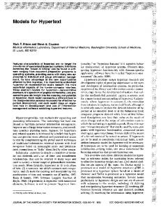
Figure 1: Comparison of Root Mean Square Error for RCM estimators of βi as T varies from √ 5 to 50. For all runs of the experiment N = 20, β = 5, γ = 1.8, σε2 = 1, and σx2 = 0.01. 17

The key issue in estimating the RCM model is separating the sampling from systematic error. Accordingly, this gets easier as the sampling error get smaller. To see this, consider the case where we knew the βi ’s for sure. We could then estimate γ by calculating its sample variance. We should expect to see all the RMSEs for all of the candidate estimators monotonically decrease as sampling error declines. Our first experiment was designed to see this effect. There are several ways to decrease the sampling variation. We choose perhaps the simple method: increase T .17 For all of the runs of the experiment, we fixed N = 20, β = 5, √ γ = 1.8, σε2 = 1, and σx2 = 0.01 and varied T over the range {5, 10, 20, 30, 40, 50}. Note that in this setup there is a fair amount of parameter heterogeneity. We should expect to see βi ’s vary from a low of about 1.4 to a high of about 8.6. If we put this in terms of an F -test of the null that the coefficients do not vary by unit, the average F -statistic over the 1000 runs with T = 20 was 1.65. This, which given our degrees of freedom, is approximately the 95% critical value for the F -distribution. Thus these simulations are, for a typical T = 20, on average, ones where researchers deciding whether to use pooled OLS or unpooled OLS would find themselves either just barely rejecting or just barely not rejecting, the null hypothesis of pooling. Since the F -statistic was not experimentally manipulated over the 1000 replications, the test statistic differed over the replications, even when T = 20. More importantly, the F -statistic is lower for smaller values of T and higher for larger values. Thus the portions of the Figure 1 where T < 20 consists largely of replications where researchers using a pre-test strategy would decide to pool; when T > 20, researchers would reject the null hypothesis of pooling.18 The results are presented in Figure 1, which graphs the RMSEs for our six proposed estimators over the six treatments. As expected RMSE declines for all of the estimators as T increases. Unit by unit OLS (and the Stein rule shrinkage estimator, which closely approximates unit by unit OLS) perform poorly for smaller T s, and only catches the pooled estimators when T > 32. Note that researchers using a pre-test strategy would stop pooling when T > 20; if they switch to unit by unit OLS at T = 20, our simulations indicate that they will have chosen an inferior strategy. We have not directly investigated the properties of a pre-test estimator (combining pooled and unit by unit OLS), but these simulations indicate that researchers should pool beyond the point where the critical 95% value of the F -statistic indicates that pooling should be rejected. While the fully pooled OLS estimator is never really strongly outperformed by any of the RCM estimators in our study, it is only better than those estimators when T < 10. At that point, both the Smith Bayesian estimator with uninformative prior and our own BKK kludge do better than pooled. OLS. Both these estimators outperform Hsaio; the latter does σ2

In our simple case Var[βi ] = T σε2 . Hence we could lower sampling variance also by decreasing σε2 or x increasing σx2 . However, since we don’t worry about the distribution of our regressors or errors much in practice we choose to look at sample size. 18 Since all the F -statistics have 19 degrees of freedom in the numerator (N = 20), and 100 or more degrees of freedom in the denominator, the 95% critical values of F range from 1.7 to 1.6. In the experiments, the average F -statistic is 1.2 when T = 5, 1.3 when T = 10, 1.65 when T = 20, 1.9 when T = 30, 2.3 when T = 40 and 2.6 when T = 50. Thus researchers using a pre-test strategy would clearly used the pooled OLS estimator until T > 20 and clearly reject pooling if T > 20. 17

18

catch up to the two other RCM estimators, but it never surpasses them.19 To better see what is happening, we can look at how the various estimators estimate γ. Since neither Stein rule nor the OLS estimators produce an estimate of γ, we only compare the three RCM estimators. This comparison is done under the identical conditions to the experiments which generated Figure 1. Figure 2 shows how the three RCM estimators perform in their estimate of γ.

Hsiao BKK Smith (MLE)

Root Mean Square Error

40

30

20

10

0 10

20

30

40

50

Number of Time Periods

Figure 2: Comparison of Root Mean Square Error for RCM estimators of γ as T varies from √ 5 to 50. For all runs of the experiment N = 20, β = 5, γ = 1.8, σε2 = 1, and σx2 = 0.01. As in Figure 1, BKK and Smith perform similarly. They both improve rapidly as T increases to 10, and then improve very slowly as T continues to grow. Both estimators outperform Hsaio, with the poor performance of Hsaio being greatest, not surprisingly, for 19

If T is large enough, then OLS sampling variance is small enough so that neglecting it, as the Hsaio estimator does, is no longer terrible. But as T gets large, the BKK kludge never has to set the γ estimate to zero to avoid a negative variance. Thus, for large T , Hsaio and BKK converge. For the conditions of this experiment, convergence occurs at about T = 30. Thus for T > 30, any of the three RCM estimators appear to be acceptable.

19

smaller T s. But Hsaio continues to do worse at estimating γ even as T grows to 50, though, as expected, the gap between Hsaio and the other two estimators decreases. To get a better idea of why the various RCM estimators perform so poorly, we present a density plot of the estimates of γ in Figure 3. These are for the case where T = 20, γ = 1 and other parameters as in the first set of experiments. We choose γ = 1 here to obtain a fairly homogeneous set of units, which is a hard case for the RCM. As can be seen almost all most all of the estimators produce a series of estimates of γ which have modes larger then the true value of 1. This can be seen most clearly for the Hsaio estimate that has no density at the true value; all of the mass is above it. Remember that Hsaio errs by assuming the sample variation of the OLS estimates to be zero; this is done to make the estimate of Γ positive definite (or in our case of a scalar γ, positive). If we simply leave the sample variance of the OLS estimates in the estimate of γ, we have another plausible estimator, suggested by Swamy. But we see that about half the time this yields a negative estimate for γ, which makes no sense (γ is a variance). Our BKK performs a bit better. The mode is below 1 and by construction has all its mass is above zero, but there is still a sizable amount of runs with very large estimates. Lastly, the Smith iterative estimator — which in this case is the ML estimate — looks the best. The mode is almost on the true value, as expected for a ML estimator, but we still see there is a lot of mass above 1. The distribution is skewed right. On these runs, which overestimate γ, we are under-shrinking and getting poor performance in all of the various RCM estimators. The surprising result from the first experiment was how well the pooled OLS performed, at least for T < 30, but with non-negligible coefficient variability. A natural question to ask is how large must the variation in βi get before pooled OLS fails because it is over shrinking the data. To explore this we ran another set of simulations similar to the first, but now we √ have fixed T = 20 and we are going to let γ vary from 0 to 5.20 The results can seen in Figure 4. As in our first experiment, an F -test of the null hypothesis that the pooled model √ is correct would be rejected when γ > 1.8. RMSEs for the various estimators (for βi ) are in Figure 4; RMSEs for estimates of γ are in Figure 5. As before, Stein rule and unit by unit OLS are very similar. While the Stein rule shrinkage estimator slightly outperforms unit by unit OLS for all values of γ, the advantage of the Stein rule over unit by unit OLS is negligible, and disappears almost completely as γ gets larger. √ Pooled OLS outperforms unit by unit OLS until γ > 2.3. As before, this is well beyond the point where pre-test oriented researchers would reject pooled OLS. Pooled OLS outperforms √ both Hsaio and Smith until γ = 1.8, which exactly where the null hypothesis of pooling √ would just barely be rejected. As γ grows beyond 1.8, the disadvantage of pooled OLS as √ compared to any of the RCM estimators grows. But as γ grows from just under 2 to 5, the advantage of the RCM estimators over unit by unit OLS declines. √ Our kludge, BKK, performs almost as well as pooled OLS when γ < 1.8, and as √ well or slightly better than the other RCM estimators when γ > 1.8.21 At least for √ The x-axis of the graph, and our discussion, is in terms of γ, that is, standard deviations rather than variances. 21 Again, as γ grows, the OLS sampling variance declines relative to γ, so the Hsaio estimator improves with γ. 20

20

0.20

0.20

0.15

0.15

0.10

0.10

0.05

0.05

0.0

0.0 -4

0

4

8

12

16

-4

0

Hsiao

4

8

12

16

12

16

Swamy

0.6

0.3

0.4

0.2

0.2

0.1

0.0

0.0 -4

0

4

8

12

16

-4

BKK

0

4

8

Smith

Figure 3: Density plots of the RCM estimators of γ for the case of N = 20, T = 20 β = 5, γ = 1, σε2 = 1, and σx2 = 0.01.

this set of experiments, BKK dominates the other two RCM estimators, with any of the RCM estimators dominating unit by unit OLS estimator. Unpooled OLS is only saved from √ domination by very homogeneous data, where γ < 1.3. But even here, the advantage of unpooled OLS over BKK is not great. While it appears that one could do well via a pretest of the null of pooling and then choosing either pooled OLS or any of the RCM estimators based on whether or not the null is rejected, one can do just about as well with BKK. Note 21

5 Unit by Unit OLS Stein Rule Hsiao Smith (MLE) BKK Pooled OLS

Root Mean Square Error

4

3

2

1

0 0

1

2

3

4

5

Standard Deviation of Beta

√ Figure 4: Comparison of Root Mean Square Error for RCM estimators of βi as γ varies from 0 to 5. For all runs of the experiment N = 20, T = 20, β = 5, σε2 = 1, and σx2 = 0.01.

that since both the pre-test estimator and BKK do not have smooth likelihoods, the exact properties of either estimator are hard to derive. The similarity of a pre-test strategy and BKK should not be very surprising, since BKK is a pre-test estimator, but one where the pre-test is hidden a bit. Turning now to the estimation of γ, the results in Figure 5 are similar to those in Figure 2. √ For large enough γ the three RCM estimators will perform similarly; but for γ < 5, the Hsaio estimator provides a much worse estimator of γ than do either of the other two RCM estimators. As previously, the performance of Smith and BKK in estimating γ is very similar. This section has only presented two sets of experiments, and clearly many more need to be done before we can draw firm conclusions about which estimators should be used. What is clear is that pooled OLS is often a good choice, even where statistical tests reject the null of pooling. It is also clear that the Stein rule shrinkage estimator we have implemented does not shrink the unit by unit OLS estimates enough. Given our experiments, BKK and Smith seem to perform well over a range of circumstances, and both seem to perform 22

12 Hsiao Smith (MLE) BKK

Root Mean Square Error

10

8

6

4

2

0 0

1

2

3

4

5

Standard Deviation of Beta

√ Figure 5: Comparison of Root Mean Square Error for RCM estimators of γ as γ varies from 0 to 5. For all runs of the experiment N = 20, T = 20, β = 5, σε2 = 1, and σx2 = 0.01.

similarly over that range. Whether this is borne out in other experiments remains to be seen.22 If it is, then researchers will have to choose between the computational simplicity 23 of BKK, but with its difficult statistical properties, versus the more computationally difficult Bayesian estimator of Smith, but one whose Bayesian heritage makes is statistical properties well understood.24 We would not want to make this difficult choice without further Monte Carlo experimentation. But at this point, these two estimators, or a pretest estimator using pooled OLS if we fail to reject pooling, appear to be the relevant competitors. While we have not examined the maximum likelihood methods of Pinheiro and Bates, the analysis 22

We should also stress that the experiments were performed under assumptions that make the best case for RCMs. We do not know, for example, how RCMs would perform if we allowed for more than one random coefficient, or if we allowed those to covary, or even how random coefficients coexist with random effects. 23 One could take the Stata ado file for its random coefficients estimator and incorporate the BKK correction in well under a day. 24 While we could kludge some standard errors for BKK, it would be hard to demonstrate their good properties other than by simulation.

23

presented in Section 2 leads us to believe that the full maximum likelihood estimator will perform similarly to Smith’s Bayesian estimator. If this is the case, we might choose the Pinheiro and Bates method since it is already nicely implemented in Splus; alternatively we might prefer the Bayesian approach because of its good heritage (and our ability to examine sensitivity of results as we change priors, a subject we return to in the conclusion).

5

Empirical application

To get some feeling for how RCMs work with real data, we look at the Garrett (1998) model of the political economy determinants of economic performance and policy, and specifically his model for the growth of GDP that we have analyzed elsewhere.25 Garrett is interested in whether the interaction of labor centralization and left control of the government predicts economic growth (so that fastest growth is observed in nations with both left governments (LEFT) and centralized labor bargaining (LABOR). In addition to these three variables (the interaction and its two linear components), he includes three economic controls, lagged growth, oil dependence and overall economic growth in the OECD (trade weighted). Garrett also includes country fixed effects and four variables indicating different interesting time periods. The model is estimated using annual data on 14 OECD countries from 1966–90, so N = 14, T = 25. Estimates of the Garrett model, without fixed effects are in Table 2. Fixed effects are omitted because it is hard, as noted above, to discern in this model whether unit to unit variation is due to variations in intercepts or coefficients. The model is estimated with straight OLS assuming full pooling.26 The economic variables have the expected sign, and the hypothesis that nations with left governments and centralized bargaining grow faster is upheld. We can examine whether the coefficients on LEFTxLABOR vary by country by moving to an unpooled model where we add the interaction of LEFTxLABOR and 13 country dummies (omitting the US) to the specification. An F -test on whether these 13 additional interactions are needed in the specification (that is, on the null hypothesis of full pooling) yields an F statistic 4.50 with 13 and 326 degrees of freedom. Since the P -value of this statistic is zero to four decimal places, we can easily reject the null hypothesis of full pooling. The OLS estimates of the βi for the LEFTxLABOR interaction coefficients are in Table 3; these are obtained by adding to the basic Garrett specification all 14 interactions of LEFTxLABOR with the country dummies while dropping the linear LEFTxLABOR term. 25

This model is analyzed in a variety of ways in Beck (2001). To get ahead of ourselves, but to be fair, in that paper, as here, we found that Japan looked different from the rest of the countries modeled, using either cross-validation or simple fixed or random effects. Here we also find that Japan is different in a coefficient of interest. While this example serves our needs for this paper, the appropriate substantive conclusion is probably that one should model Japan separately, rather than use an RCM. But the RCM analysis presented here is relevant to some points we make in this paper. 26 We not use PCSEs since we not now know how to incorporate PCSEs into the RCM framework. This is an illustration of Stimson’s law, that one can solve only one interesting methodological problem in any given analysis.

24

Table 2: Garrett model of economic growth in 14 OECD nations, 1966–1990 OLS Variable GDPL OIL DEMAND LABOR LEFT LEFTxLABOR PER6673 PER7479 PER8084 PER8690 CONSTANT

βˆ .25 −3.68 .37 −.65 −.95 .26 1.29 −.05 −.62 −.17 3.68

SE .05 4.36 .10 .28 .35 .11 .58 .59 .61 .59 .89

Table 3: Comparison of estimated unpooled and random coefficient of LEFTxLABOR by country, Garrett model of economic growth in 14 OECD nations, 1966–1990 Unpooled Country US Canada UK Netherlands Belgium France Germany Austria Italy Finland Sweden Norway Denmark Japan a

βˆi .52 .40 .13 .07 .17 .32 .32 .28 .37 .36 .24 .29 .23 1.65

SE .43 .34 .28 .30 .24 .51 .22 .17 .23 .21 .18 .21 .20 .38

RCMa βˆi .00 −.01 −.19 −.23 −.14 −.06 −.01 .00 .05 .04 −.05 −.01 −.07 .69

Deviations from βˆ = .26, SE= .11 SE of random effects is .24

25

None of the coefficients, other than for Japan, are statistically significant. Clearly the coefficient for Japan is larger than that of the other countries, and the other countries appear to have relatively homogeneous coefficients. Note that the non-Japan coefficients are not generally smaller than the coefficient in the fully pooled model; rather the standard errors in the unpooled model are large (because of multicolinearity) and hence it is hard to say much about these coefficients. Thus the unpooled analysis tells us that the Japanese coefficient on LEFTxLABOR is considerably larger than any of the other country’s coefficient on that variable, and little else. The random coefficients model, which assumes that βi = β + γi , where γi is independent of all the model variables seems like it might solve the multicolinearity problem. An RCM, with only the coefficient on LEFTxLABOR being random, was estimated using the Pinheiro and Bates REML routines in Splus6.27 The RCM estimate for the mean LEFTxLABOR coefficient is .26 with a standard error of .11. This estimate is almost identical to the corresponding OLS estimate.28 The estimated standard deviation of the random coefficients around this mean is .24 (with a confidence interval of .11 to .51). A test of whether we can reject the null hypothesis of the pooled model against the alternative of the RCM (which has one additional parameter) allows us to reject the null that all coefficients are fixed with a likelihood ratio statistic of 6.23; with one degree of freedom, this yields a P -value of just over .01. The right column of Table 3 contains estimates of the deviations of the country coefficients from the overall mean β; since these deviations are assumed to be draws from the same normal with zero mean and standard deviation .24, they can be evaluated by common normal methods. As in the unpooled model, all the country coefficients appear homogeneous except that of Japan, which is considerably higher than the other country coefficients. The difference between the Japanese coefficient and the others is both statistically and substantively significant. What can we say based on this one example?29 Either analysis tells us that Japanese coefficient is much larger than the others, with the RCM “shrunk” coefficient being a somewhat smaller than the unshrunk unpooled OLS coefficient. The RCM has the advantage of being able to examine coefficient variation across countries while still allowing for estimation of the overall mean effect. This is a nice advantage. But the advantage here is not great; either approach tells us that one country’s coefficient is out of line with the others. But the clumsiness of the unpooled model (and the inherent multicolinearity problems with estimates from that model) do mean that it would be nice if we had a workable way of 27 Results were similar, but not identical with full maximum likelihood, with statistics varying by about 10% between the two methods. We used the SPLUS6 routines not because we know they are good, but because our simulations indicate that the Hsaio based routines in both Stata and LIMDEP are not very good. The Splus6 procedures are also very flexible, and would be chosen over LIMDEP or Stata even if they were computationally similar. 28 Even if we think the RCM model is correct, the OLS estimate of the pooled β yields consistent, although not fully efficient, estimates of the mean β of the random coefficient distribution. 29 This example is far from ideal, since Japan does not fit the overall model in many ways. We have searched for other examples, but have found no especially compelling examples where RCMs produce stunning results. We would be happy to hear of examples where RCMs are useful, or to receive TSCS data sets where analysts think they might be useful.

26

estimating RCMs. The Monte Carlo analyses of the previous section, however, indicate that this is not a trivial problem.

6

Conclusion

There is little doubt, as Western noted, that the RCM should appeal to comparativists who are not so naive as to assume that all countries are identical but who are sufficiently committed to statistical analysis that they cannot assume that all observations are sui generis. The RCM appears to offer the analyst a flexible middle position. And it appears as though we can allow the data to tell us just how heterogeneous the units are. As noted, there is only one political science application of RCMs to TSCS data (that we know of), and that one appears to be largely for didactic purposes. So we must ask why RCMs have seen so little usage, and then, should they be used more? We stress that we only deal here with TSCS data and make no claims about either panel data or the fractional pooling approach recommended by Bartels (or about Bayesian approaches in general). Our Monte Carlo analysis indicates that the assumption of pooling leads to reasonably good estimates, not just of the overall model parameters, but also of the individual unit parameters. When there is a lot of unit to unit parameter heterogeneity the pooled model does become inferior. But it takes a non-trivial amount of heterogeneity before this happens. Taking advantage of the law of large numbers and the central limit theorem is a good thing, and the pooled model surely does that. Obviously with enough information, the unit by unit estimates become good, but it takes an atypical amount of information before that becomes the case.30 The Monte Carlo analyses reported also indicate that standard GLS based RCM estimators, the ones implemented in some common packages used by political scientists, perform poorly. Since most political scientists use standard packages, there is every reason to believe that those who have tried RCMs using, say, Stata or LIMDEP have given up because the RCM estimators in those packages perform so poorly. Our simulations indicate the a Bayesian estimator, using uninformative priors, or a kludge of our own, seems to perform well in our experiments. Whether that will hold up in future experiments remains to be seen. If the Bayesian estimator performs well, we would also expect maximum likelihood based estimators to perform well, since the Bayesian estimator of Smith is essentially maximum likelihood. But at present this is speculation. Finally, even if comparativists are not so naive as to assume complete homogeneity, those who do statistical analysis usually believe that the units under analysis are probably not too heterogeneous (whatever that means). And they clearly understand the benefits in both interpretation and reporting of pooled models over their not fully pooled brethren. Thus, for example, the gains from using a fully pooled model would, to our minds, justify a pre-test estimator where we first test the null of homogeneity and then estimate a fully pooled model unless that null hypothesis is rejected. But, as we have seen, the shrinkage type estimators 30

This is consistent with our reported in Beck and Katz (1996b) that it is better to assume a homogeneous autoregressive process rather than estimate separate processes for each unit unless there is an enormous amount of unit to unit variation in those processes.

27

(and we presume most other classical and empirical Bayes estimators) shrink much less than we imagine a typical comparativist would like. In situations where comparativists should usually be happy to pool, the RCM estimators appear to shrink unit by unit OLS estimates much less than we might like. A solution to this problem may be that we have to allow ourselves more judgment. If we as political scientists really believe that the units are relatively homogeneous, we can impose that in our priors. But if move from being either empirical Bayesians or Bayesians with very gentle priors, we of course run the risk of others doubting our work because they disagree with our priors. The solution here, as suggested by Bartels, is that we provide a variety of results, allowing our priors to vary. It may be that the Bayesian estimates vary a lot with choice of prior, in which case we have to worry about which prior we believe. But it may be the case that over a wide range of priors, which many analysts would accept, we would find roughly similar conclusions. This is surely an avenue worth exploring. RCMs may require more judgment than either classical or data driven Bayesian methods allow for. But that conjecture must be for another paper.

References Alvarez, R. Michael, Geoffrey Garrett and Peter Lange. 1991. “Government Partisanship, Labor Organization, and Macroeconomic Performance.” American Political Science Review 85:539–56. Anselin, Luc. 1988. Spatial Econometrics: Methods and Models. Boston: Kluwer Academic. Bartels, Larry M. 1996. “Pooling Disparate Observations.” American Journal of Political Science 40:905–42. Beck, N. 2001. “Time-Series–Cross-Section Data.” Statistica Neerlandica 55:110–32. Beck, Nathaniel and Jonathan N. Katz. 1995. “What To Do (and Not To Do) with TimeSeries Cross-Section Data.” American Political Science Review 89:634–47. Beck, Nathaniel and Jonathan N. Katz. 1996a. “Lumpers and Splitters United: The Random Coefficients Model.” Paper presented at the Annual Meeting of the Society for Political Methodology, Ann Arbor, July. Beck, Nathaniel and Jonathan N. Katz. 1996b. “Nuisance vs. Substance: Specifying and Estimating Time-Series–Cross-Section Models.” Political Analysis 6:1–36. Bryk, A. S. and S. W. Raudenbush. 1992. Hierarchical Linear Models, Applications and Data Analysis Methods. Thousand Oaks: Sage. Franzese, R. J. N.d. The Political Economy of Macroeconomic Policy in Developed Democracies. New York: Cambridge University Press.

28

Garrett, Geoffrey. 1998. Partisan Politics in the Global Economy. New York: Cambridge University Press. Hildreth, C. and C. Houck. 1968. “Some Estimates for a Linear Model with Random Coefficients.” Journal of the American Statistical Association 63:584–95. Hsaio, Cheng. 1986. Analysis of Panel Data. New York: Cambridge University Press. Iversen, Torben. 1999. Contested Economic Institutions: The Politics of Macroeconomics and Wage Bargaining in Advanced Democracies. New York: Cambridge University Press. James, W. and C. Stein. 1961. Estimation with Quadratic Loss. In Proceedings of the Fourth Berkeley Symposium on Mathematical Statistics and Probability. Vol. I pp. 361–79. Judge, G. and M. Bock. 1978. The Statistical Implications of Pre-Test and Stein Rule Estimators in Econometrics. New York: North-Holland. Judge, George, W. E. Griffiths, R. Carter Hill, Helmut L¨ utkepohl and Tsoung-Chao Lee. 1985. The Theory and Practice of Econometrics. Second ed. New York: Wiley. Maddala, G. S. and Wanhong Hu. 1996. “The Pooling Problem.” In The Econometrics of Panel Data, ed. L. M´aty´as and P. Sevestre. 2nd ed. Dordrecht: Kluwer Academic pp. 307–22. Pinheiro, Jos´e C. and Douglas M. Bates. 2000. Mixed Effects Models in S and S-Plus. New York: Springer. Smith, A. F. M. 1973. “A General Bayesian Linear Model.” Journal of the Royal Statistical Society, Series B 35:67–75. Snijders, Tom and Roel Bosker. 1999. Mulilevel Analysis. Thousand Oaks: Sage. Swamy, P. A. V. B. 1971. Statistical Inference in Random Coefficient Models. New York: Springer-Verlag. Western, Bruce. 1998. “Causal Heterogeneity in Comparative Research: A Bayesian Hierarchical Modelling Approach.” American Journal of Political Science 42:1233–59.

29