R. R. Martin. Department of Computer Science, Cardiff University,. PO Box 916, 5 The Parade, Cardiff, CF24 3XF, UK,. {B.I.Mills, F.C.Langbein,Dave.Marshall ...
Approximate Symmetry Detection For Reverse Engineering B. I. Mills
F. C. Langbein
A. D. Marshall
R. R. Martin
Department of Computer Science, Cardiff University, PO Box 916, 5 The Parade, Cardiff, CF24 3XF, UK, {B.I.Mills, F.C.Langbein,Dave.Marshall, Ralph.Martin}@cs.cf.ac.uk.
Abstract The authors are developing an automated reverse engineering system for reconstructing the shape of simple mechanical parts. B-rep models are created by fitting surfaces to point clouds obtained by scanning an object using a 3D laser scanner. The resulting models, although valid, are often not suitable for purposes such as redesign because expected regularities and constraints are not present. This information is lost because each face of the model is determined independently. A global approach is required, in particular one that is capable of finding symmetries originally present. This paper describes a practical algorithm for finding global symmetries in suitable B-rep models built from planes, spheres, cylinders, cones and tori. It has been implemented and used to determine approximate symmetries of models with up to about 200 vertices in reasonable time. The time performance of the algorithm in the worst case is bounded by O(n3.5 log4 n), and a justification is given that on common engineering objects it takes about O(n2 log4 n), making it a practical tool for use in a reverse engineering package. Details of the algorithm are given, along with some results from a number of illustrative test runs. Keywords: Beautification; Approximate Symmetry; Reverse Engineering; Geometric Interrogations and Reasoning.
1 INTRODUCTION Reverse engineering is a topic of current interest in computer-aided design [13]. Here we take it to mean generating a boundary representation CAD model of the shape of a mechanical component. Unlike conventional engineering, which begins with a description of what the part should do, and produces a geometric model suitable for manufacturing, reverse engineering begins with the manufactured part itself and produces a geometric model [13]. This process involves scanning the surface of the object in order to produce a solid model. The authors’ current project concerns B-rep models that have been derived from fitting surfaces to a point cloud obtained using a commercial 3D laser scanner. The B-rep model is constructed using previously developed software [2]. This software produces a model with natural faces. For example, processing clean data from a cube produces a model with six planar faces, twelve straight edges, and eight vertices. However, Sixth ACM Symposium on Solid Modelling and Applications, Ann Arbor, Michigan, June 4 – 8, 2001. c ACM 2001, 1-58113-366-9/01/06. Copyright This version is posted by permission of ACM and is limited to personal use only and may not be redistributed. The official version is available at the ACM Digital Library.
due to the response of the algorithms to noise in the data, and the fact that the faces are fitted individually, even if a perfect cube is scanned, the resulting faces and edges are not typically parallel and orthogonal. It is also possible that a single square face might be incorrectly interpreted as two triangular faces, adding a new edge on the diagonal. The current project considers objects with only planar, spherical, cylindrical, conical and toroidal surfaces that either intersect at sharp edges or are connected by fixed-radius rolling ball blends. It has been shown [10] that many mechanical components can be described by these surfaces, and algorithms are available [9] that reliably determine these faces from point clouds. The long term goal of the current project is to produce a system that will modify the parameters of these surfaces to produce a model that is more suitable for redesign. The model can be improved, for example, by adjusting it so that it becomes exactly symmetrical where before it was only approximately so, by lining up parts that lie in almost the same direction, and by making repeated features exactly congruent. This process of model improvement is called beautification. Part of the information required for beautification of the model is obtained from the approximate symmetries of special points on the surface of the object. This paper shows how to find these approximate symmetries. A polyhedron is completely determined once the geometric and combinatorial information about the vertices is known. The geometric information is the location of each vertex. The combinatorial information1 indicates which vertices are on a common edge, and which are on a common face. The symmetries of the polyhedron are exactly those symmetries of the points which preserve the combinatorial information. When the faces are curved, other points, such as the centroids of faces, or their centres of curvature, need to be used as well, to maintain the relationship between the symmetries of the points and the symmetries of the object. This paper only deals with finite symmetry groups. The case of infinite symmetry groups is covered in other work by the same authors [7]. Any bounded single sheet surface with an infinite number of geometric symmetries must be a (possibly composite) surface of revolution. Of these, only the sphere has more than one axis of continuous rotational symmetry. We are considering only objects made from planar, spherical, cylindrical, conical and toroidal surfaces. The axes of any cones, cylinders and tori will be coincident. The planes will be perpendicular to all these axes. Any centres of spheres, centres of tori and apices of cones will lie on a single line. The detection of these characteristic regularities has been considered separately. Practical algorithms are presented in another paper [7]. These methods can be included as a preprocessing stage for the algorithm presented in the current paper. For the finite symmetry groups, the symmetries of the object as a whole are also symmetries of certain sets of points derived from the object, for example, the set of vertices of the object, the set of centres of spheres, the set of centres of tori, the set of centroids of the faces and the set of centroids of the edges. For non-collinear collections of points the number of symmetries is bounded by twice 1 more often called ‘topological’ information in solid modelling literature
the number of points or 120 [8], whichever is the larger. So, first we generate the symmetries of the set of points, and then we retain only those that preserve the type of each point (vertex, centroid of a torus, etc.), the adjacency, and the orientation information stored in the model. Each of these tests takes constant time per permutation per point. So, with only linear amounts of extra work this approach generates exactly the symmetries of the whole B-rep model from those of the points. The symmetry of the object is not always reflected in the symmetry of the B-rep model. For example, when a sphere is modelled as two half spheres joined at the equator, symmetries of the B-rep model must preserve the equator. Because of this the algorithm has two stages. The first stage is a partial solution to the problem of adjusting the structure of the model so that it reflects the symmetries of the object. This stage determines ways of grouping and identifying points to obtain new collections. It determines all the ways of grouping the points subject to constraints that are made clear in this paper. The second stage determines the approximate symmetries of each of the new collections. The input to the whole algorithm is a list of points, and the output is a collection of adjusted point lists each paired with a list of permutations expressing the symmetry of that model (the nature of the adjustment is explained later on). An explicit example of this is given in Section 3, including the the input data, and an explanation of the output. Following this, adjusting the equations of the surfaces to fit the new centres and vertices can be done by standard geometry. The aim of the project is to develop algorithms and heuristics that can generate an ideal model of an observed object. The model must conform exactly to regularities only approximately present in the object. Several interpretations of the requirement are discussed in this paper. Some regularities are related to decomposition of the object into congruent parts, such as cutting a cube into octants, and a long prism being cut into a number of slices. Other regularities are not so directly related to the shape of the object, but to computable properties of the object. These properties include directions along edges and orthogonal to faces or the axis of a cylinder, cone or torus. Special points such as the centre of a sphere, the apex of a cone, and the centre point of a torus are also interesting. These lines and points may be coincident, parallel, coplanar, co-cylindrical and so on. The computing of related regularities is a subject on its own, as discussed in [7]. The rest of this paper concentrates on the determination of symmetries of collections of points. In particular, a number of definitions put forward in the literature are discussed in the current context, our algorithm is described and analysed in some detail, and empirical performance and time complexity are presented. Finally there is a brief discussion of the significance and future development of the algorithms.
threshold or (2) the time requirements of the algorithm. The reason for the latter is illustrated by the sock matching problem. If a number of paired grey socks are mixed together, a direct attempt to pair them might start by pairing two of similar but different shades. The problem might not be discerned until eventually a black sock and a white sock are all that are left. The problem with this approximate matching of the socks is a global phenomenon, requiring knowledge of the entire collection. The specific problems with the three definitions are discussed below. Zabrodski [16] considers the problem of constructing a measure of approximate symmetry for molecules. The elements of the object may be seen as coloured points. The motivation is to determine a numerical quality of molecules that can be related to things such as melting temperature of solids. The distance between two collections of points is defined as the root mean square distance between the individual points of closest approach. The symmetry measure is the distance between a set and its transforms according to the ‘most likely’ symmetry group. In defining the most likely group Zabrodski makes use of orbits of group actions, but only for mirror symmetry and rotation taken individually, and does not generalize this to an arbitrary symmetry group. However, in our paper general symmetry groups are considered. Zabrodski’s work is interesting, but aimed mainly at continuous measures of symmetry, rather than determining whether or not that symmetry exists. With a continuous measure the distinction between symmetric and asymmetric disappears and arbitrary thresholds must be chosen. In Zabrodski’s scheme a triangle is at least somewhat like a square. This is not a robust solution to the problem of finding the intended symmetry in a physical object. Iwanowski [5] considers the difficulty of determining the existence of a nearby collection of points with a specified symmetry. The notion of neighbourhood used here is that two collections are close to each other if there is a one-to-one correspondence between them such that the distance between corresponding points is less than a specified tolerance. Iwanowski shows that this problem is NP-hard even when limited to two dimensions. At the end of the paper Iwanowski suggests that this work might be sped up in practice if we could assume that the orbits are already known. This begs the question. The algorithm presented in our paper could also be made much faster if the orbit structure was already known, but when we begin fully automated search we do not know what it is, and it can take some time to determine it. Our algorithms use a different definition, which leads to a much faster implementation. Iwanowski’s work is significant in two respects. Firstly, he emphasises that the approximate problem can be much harder than the exact problem, and secondly, the question can be paraphrased as asking whether the object can be made symmetric by changes to within a given tolerance. This is the style of question which the current paper considers. However, Iwanowski’s work is too exacting, and the difficult cases are not of interest in the analysis of physical objects. Alt [1] considers a different definition. An approximate symmetry is not specifically referred to a symmetric object. He determines whether an isometry can be found that maps the points of the collection close to themselves, in a one to one fashion. The notion of closeness is essentially that of Iwanowski, but the set is compared with a transformed version of itself, rather than an example of a perfectly symmetric collection. This definition is significant in relation to this paper since the basic idea of the correspondence is the same. Alt’s definition of symmetry seems as intuitively justified as Iwanowski’s definition, but it is easier to compute. Nevertheless for general symmetry in the plane Alt’s method still takes time O(n6 ). Alt’s work is related to ours by the similar definition of approximate symmetry, but like Iwanowski’s work the emphasis is on finding a given symmetry to a given tolerance. We are firmly committed to the idea that neither the symmetry nor the tolerance should be predetermined. Our algorithm deter-
2 PREVIOUS WORK The case of determining exact symmetry has been well studied. Sugihara [11] considers congruence of polyhedra, Jiang [6] considers simple algorithms for polyhedral symmetry, and Wolter [14] considers optimal algorithms for polyhedra in three dimensions. These researchers show that polyhedral symmetry can be determined in three dimensions in O(n log n) time (where n is the number of vertices) by the use of symbolic sorting algorithms. However, in practice, these results do not transfer to the approximate case because they require the ability to tell locally whether one point can be mapped to another. In the approximate case the decision has to be a global one based on the behaviour of the entire object. Approximate symmetry can be defined in more than one intuitively acceptable manner. Three central definitions exist in the literature, each of which is difficult to use for the beautification problem because of (1) the requirement to determine an arbitrary
2
( 0.90 ( 1.00 ( 1.00 ( 1.00 ( 1.10 ( 1.00 (-1.00 (-1.10 (-1.00 (-1.00
mines maximal symmetry, and the level of tolerance that will generate it. The difficult cases in previous work relate to problems in determining the existence of precisely, no more and no less, the symmetry being sought. In this paper, with an emphasis simply on finding the maximal symmetry, the pragmatic problem of finding regularity in the object is solved, and the difficult cases involving ambiguity in matching points are avoided. Another approach entirely warrants mentioning at this point. The thesis of Tate [12] describes an implementation of an algorithm for determining partial symmetry. The idea is to match every pair of edge loops and find the isometries that relate the two, and then to group these isometries according to similarity. The actual implementation only checks for axes of continuous rotation, and mirror planes. The result is an algorithm that is expressed by Tate as between O(n2 ) and O(n4 ), where n is the number of loops. Test runs show, for example, that 188 loops take 72 seconds on a 200Mhz Pentium. There are more loops than faces, but in general there would be typically a limit to the number of loops per face, such that the number of loops and the number of vertices are of the same order. Comparisons of Tate’s results with ours in Table 1 show that her algorithm runs a few times faster for a couple of hundred points. Comparison of theoretic complexity suggest a similar order. However, the two algorithms are not computing the same thing. Tate’s algorithm computes partial symmetries and runs faster, but the order is the same within the ability to test this, and Tate’s algorithm as implemented admits less isometries as potential symmetries. Our algorithm uses all possible isometries, as implemented, and detects approximate symmetries. Tate has no definite strategy for the detection of approximate symmetries other than to try the same thing with lower tolerance. Our algorithm comes complete with a direct means of computing a rectified (i.e. symmetric) object, while Tate’s is interested in finding gripping positions, and mainly refers to rectification generically rather than having a distinct strategy. In summary, the two algorithms compute different but related things, of possibly similar difficulty, in similar times. They appear to be complimentary rather than working on the same thing.
1.00 0.90 1.00 1.00 -0.90 -1.00 1.00 0.90 -1.00 -1.00
1.00) 1.00) 0.90) -1.00) 1.00) -1.00) 1.10) -1.00) 1.00) -0.90)
# # # # # # # # # #
0 0 0 1 2 3 4 5 6 7
Figure 1: The Input Vertices Approximately on a Cube ( 0.97 ( 1.00 ( 1.10 ( 1.00 (-1.00 (-1.10 (-1.00 (-1.00
0.97 1.00 -0.90 -1.00 1.00 0.90 -1.00 -1.00
0.97) -1.00) 1.00) -1.00) 1.10) -1.00) 1.00) -0.90)
# # # # # # # #
0 1 2 3 4 5 6 7
Figure 2: The Vertices after the Algorithm’s First Stage �
� �
� �
� �
�
� �
�
�
�
�
�
�
�
�
�
�
� �
�
� �
�
�
� �
�
�
�
�
�
�
�
�
� �
�
!
�
�
"
" #
#
�
!
�
� �
�
�
�
�
�
�
�
�
�
�
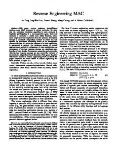
Figure 3: Input (left) and Output (right) of the First Stage
a permutation. The vertices are rearranged by the symmetry. The second stage of the algorithm determines the set of permutations induced by approximate symmetries of the collection of points. In the example given there are 48 approximate symmetries. The first eight permutations are listed in Figure 4 as sets of ordered pairs. For example (0, 4) means that the point labelled 0 is moved to the location of the point labelled 4. These permutations not only map vertices to vertices, but also implicitly (by mapping end points) edges to edges. The length of an edge is adjusted to the average length of the edges that it can be mapped to. Then the entire cube can be reconstructed using triangulation to determine the location of each vertex. The resulting structure has the geometric symmetry determined by the group of permutations.
3 ALGORITHM OUTLINE Before we give a detailed explanation of the algorithm, we outline the principles using a simple example. In the following example, ten points are roughly at the corners of a cube, but one corner has three points near it (see Figures 1 and 3). The first part of the algorithm replaces certain groups of points by their centroid. The second part finds the approximate symmetries of the collection of points remaining after this grouping. If the positions in the example are considered exactly then the points are not in symmetrically related locations. However, the three points labelled 0 are much closer to each other than to the other seven points. If these are grouped as a single point then the set of points are approximately located at the eight corners of a cube (see Figures 2 and 3). The first stage of the algorithm looks for tolerance levels for which the grouping of points is consistent. The exact value of this tolerance is not important. It is only required that there exists some level of tolerance that produces the grouping. In this example the first stage determines that the three points labelled 0 could be treated as one, thus making a total of 8 rather than 10 points. The overall algorithm determines a small number of such groupings dependent on the structure of the object. Each grouping of points is examined for approximate symmetry. In this example three groupings were returned: (1) the approximate cube, (2) a grouping in which each point was on its own, and (3) the grouping into a single group containing all the points. If the approximate cube is rotated so that it comes into correspondence with itself, then each corner will be moved near to the old location of some (other, or possibly the same) corner. This induces
4 THE ALGORITHM We now describe the algorithm in detail. Pseudo code for the first and the second stage of the algorithm is presented as Algorithms 1 and 2 respectively. We assume that various abstract data types such as points, graphs, sets, partitions and priority queues are available [15]. In the pseudo-code the priority queue automatically sorts the pairs of points placed on it, so that the pair with the least distance of separation is placed at the head of the queue and will come off first. The input to the first stage of the algorithm is a list of points, and the output is also a list points, the centroids of the classes of some partition of the input list (Algorithm 1, line 19). The major task of the first stage is to compute the partition. During this process a dis-
3
00: 01: 02: 03: 04: 05: 06: 07: 08: 09: 10: 11: 12: 13: 14: 15: 16: 17: 18: 19:
First_Stage of (Points : set of point) :Q : priority_queue based on distance() = empty_queue G : graph of points = empty_graph P : grouping of points = {{X} for X in Points} for each X in Points for each Y in Points push (X,Y) onto Q while(Q is not empty_queue) pop Q into Pair add Pair to G merge group containing left of Pair with group containing right of Pair in P if distance(top of Q) > distance(Pair) and each of components of G is complete graph then Second_Stage of {centroid of S for S in P} Algorithm 1: First Stage Pseudo Code for Generating Lists of Points
1: 2: 3: 4: 5: 6: 7: 8:
(0,4)(1,0)(2,5)(3,1)(4,6)(5,2)(6,7)(7,3) (0,2)(1,0)(2,3)(3,1)(4,6)(5,4)(6,7)(7,5) (0,1)(1,0)(2,5)(3,4)(4,3)(5,2)(6,7)(7,6) (0,2)(1,0)(2,6)(3,4)(4,3)(5,1)(6,7)(7,5) (0,4)(1,0)(2,6)(3,2)(4,5)(5,1)(6,7)(7,3) (0,1)(1,0)(2,3)(3,2)(4,5)(5,4)(6,7)(7,6) (0,3)(1,7)(2,1)(3,5)(4,2)(5,6)(6,0)(7,4) (0,6)(1,7)(2,4)(3,5)(4,2)(5,3)(6,0)(7,1)
varied from just above one distance on the list to just below the next, no change in the grouping of points will occur. But as the tolerance passes each distance on the list, it is possible that the grouping will change. Thus only tolerances corresponding to these distances need to be considered explicitly.
4.1 The First Stage – Generation Of Lists Of Points
Figure 4: Output of the First Eight Approximate Symmetries
Given an input list of points, the first stage generates the list of unordered pairs of these points (Algorithm 1, line 06), and sorts that list in order of increasing distance apart. A partition of the points is initialized (Algorithm 1, line 04) so that it classes each point as distinct. A graph is also initialized to the empty graph. The connected components of the graph are the classes of the partition. The number of nodes and edges in each connected component is stored, as well as a global count of the number of components that are not complete subgraphs. (When each connected component is a complete subgraph the graph represents a consistent grouping). In this way the operations indicated in the pseudo code are quite efficient. The initial counts are zero edges and one node for each of the classes, with a total count of zero incomplete components. A tolerance level is implied, initially being zero, but no storage of this value is required. To increase the tolerance, the pairs are taken from the sorted list one at a time (Algorithm 1, line 12). If the current pair has both points in the same class, then both the edge and node counts for the component of the graph are incremented. A class is a complete graph if and only if the number of edges is equal to m(m − 1)/2 where m is the number of points. So, if the status of this equality changes, then the global count of incomplete subgraphs is adjusted accordingly. If the current pair has points in distinct classes, then these classes are merged, and the counts adjusted appropriately. The tolerance is nominally half way between the current distance and the next distance to be added. From the tolerance analysis we obtain a number of tolerance levels and corresponding consistent groupings of points. The collection of centroids of these groups is then subjected to symmetry analysis in stage 2. Each point in the new collection is the centroid of a cloud of points from the old collection. Each point in the cloud is no further from the corresponding centroid than the tolerance. Since the grouping is consistent, each point in a cloud is closer to
tance known as the level of tolerance is also determined implicitly as explained later (see Section 4.1). The first stage actually computes a number of output lists (Algorithm 1, line 17). For each of these it calls the second stage to determine what the symmetries are (Algorithm 1, line 19). The physical significance of the level of tolerance is clearest when motions of the collection of points are considered. A rigid motion of the collection that moves each point onto another is an exact symmetry. An approximate symmetry is a rigid motion that moves each point to within the tolerance of its nominal target. If in the original collection two points are within the tolerance of each other then no movement at all is required to bring the one approximately onto the other. In this case the two points within tolerance of each other are treated as being at the same location. But if three points are close to each other so that the first is within tolerance of the second and the second within tolerance of the third, it is possible that the first will not be within tolerance of the third. In this case it is not possible to consistently decide whether multiple points are in the same location. However, for each collection of points there are intervals of levels of tolerance such that the grouping of points is consistent, at least for all the points in that collection. It is only those levels of tolerance that are consistent that need to be considered. Multiple entries in the input list of points that are identical should be replaced by a single entry. When a non-zero level of tolerance is used, groups of points that are within tolerance should be replaced by a single point. The first step in the algorithm is to determine those levels of tolerance for which such replacement is consistent. Given a sorted list of the distances that occur, as the tolerance is
4
00: 01: 02: 03: 04: 05: 06: 07: 08: 09: 10: 11: 12: 13: 14: 15: 16: 17: 18: 19:
Second_Stage of (M : set of point) :i : integer X[0 .. size of M] : point Y[0 .. size of M] : point X = [centroid of M | list of M] i = maximal j in [1 .. size of m] for length(X[0 .. 0],X[j]) swap X[1] with X[i] i = maximal j in [2 .. size of M] for area(X[0 .. 1],X[j]) swap X[2] with X[i] i = maximal j in [3 .. size of M] for volume(X[0 .. 2],X[j]) swap X[3] with X[i] Y[0] = X[0] for each Y[1 .. 3] in permutations size 3 of X[1 .. size of M] backtrack Y[1 .. 3] when not preserve(Y) if extend(Y,X) output(Y) Algorithm 2: Second Stage Pseudo Code for Symmetry Analysis
point occurs at most once as a first element, and at most once as a second element. Such a list is a partial injection. Partial injections form a tree. The root of this tree is the empty list and the children of any given partial injection are those obtained by appending one more pair to the list. The permutations are the leaves of the tree. A partial injection is approximately distance preserving if the absolute difference between the separation of two given points, and the separation of their images, under the partial injection, is less than the tolerance. Most of the partial injections of the points are not approximately distance preserving. A proto-symmetry is a partial injection that is approximately distance preserving. Protosymmetries form a subtree of the partial injection tree. The approximately distance preserving permutations are exactly the maximum depth leaves of this subtree, the other leaves being protosymmetries that cannot be extended. This subtree is typically much smaller than the full tree of partial injections. To scan just the tree of proto-symmetries, in order to find all the leaves of this tree, a scan of the larger partial injection tree is conducted in a depth first manner, backtracking whenever a node is found not to be a proto-symmetry. In the pseudo code, extend adds an element onto the current tree, extending its depth, and backtrack goes up a level if adding an element creates an nonproto-symmetry. Practice, and some theoretical considerations, indicate that this approach considerably decreases the number of permutations actually considered during execution of the algorithm. Section 5 gives a discussion that indicates the worst case and expected running time in Euclidean three dimensional space for this algorithm. Also discussed are a number of symmetry concepts, and some modifications to the algorithm to help ensure that the theoretical performance is achieved in practice.
the centroid of the cloud than it is to the centroid of any other cloud. So a tolerance of half the minimum distance between any two centroids will generate the same grouping as the tolerance used by the algorithm in determining the grouping. This tolerance is used in the symmetry analysis. Classing two points as the same only when the distance between them is strictly less than this tolerance means that every point in the space is close to at most one point in the collection. It is certain that there is no ambiguity in the approximate matching of points under an isometry. An example of the input, and one of the corresponding outputs has already been given in Figures 1 and 2.
4.2 The Second Stage – Symmetry Analysis The symmetry analysis stage (Algorithm 2) of the algorithm determines the set of all permutations of the points that preserve the distances between points to within the tolerance level selected by the first stage. The pseudo code shows two major sections. Firstly, a list of points consisting of the centroid of the input points, three special input points on the convex hull of the input points, which form a non-degenerate tetrahedron together with the centroid, followed by the remaining input points is constructed (Algorithm 2, lines 06– 13). The location of these three points and the centroid determines the location of all the points in the collection, so, once the mapping of these points is established, the mapping of all the other points follows directly. Secondly (Algorithm 2, line 17) a limited depth first search of a tree of permutations is performed. Once a depth of four has been obtained (i.e. the tetrahedron has been mapped) the search proceeds by an alternative extension process, which checks if all other points are consistently mapped (Algorithm 2, line 19). The motivation for the structure of this code is efficiency. The most robust algorithm is to simply try every permutation, but this is prohibitive of resources. The operation of the actual code is explained in the rest of this section, and Section 5 which derives the complexity. A permutation is a list of pairings of the points in the collection. The action of the permutation is to take the first element of each pair and move it to the corresponding second element. In a permutation each point occurs exactly once as a first element and exactly once as a second element. A list of pairs is a part of a permutation if each
5 PERFORMANCE ANALYSIS Our algorithm is presented as two routines the first of which is a loop which sometimes calls the second, which is also a loop. In order to estimate the time taken it is sufficient to know how long the outside loop takes on the assumption that the inner loop takes no time, how long the inner loop takes, and the number of times the inner loop is called. The conclusion is that the inner loop has a time complexity of O(n2.5 log4 n) where n is the number of points. The inner loop can be expected to be called at most O(n) times, and
5
Name penta cube1 cube2 cubeoct1 icosa1 cubeoct2 tcube snubcube icosido1 icosido2 icosido4 icosido3 icosido5 icosido6 prism60 prism50 rhombix
Time (sec)
Points
0.02 0.07 0.09 0.15 0.39 0.60 2.92 3.38 5.66 5.88 6.87 7.11 24.88 64.45 165.76 401.31 831.52
5 8 10 12 14 24 24 24 30 32 36 34 74 148 180 250 120
Symmetries (5:10) (4:2) (3:6) (8:48) (10:6) (8:48) (12:48) (14:1) (13:1) (12:120) (24:48) (8:48) (24:48) (16:16) (24:24) (12:48) (30:120) (18:24) (32,31:1) (30:120) (37,36,31:1) (30:120) (34,33,32,31:1) (30:120) (74,73,68,67,66,62,61:1) (60:120) (148,110,105,104,99,98,97,91:1) (90:120) (180:240) (156,132:16) (120:120) (104:8)
Table 1: Time Taken and Symmetry Found for Sample Input Shapes also O(n2 log n) since m ≤ n. This gives us the time taken for the outer loop itself, and the time taken for the inner loop each time it is called. Since the inner loop takes a greater order of time, the time for the entire algorithm is the product of the time for the inner loop and the number of times the inner loop is called. This is O(n2.5 log4 n) × O(n) = O(n3.5 log n). Each time the inner loop is called the outer loop has made the partition of points coarser. So the immediate limit to the number of calls is n, the number of points. This limit can be reached by a collection of points built up one at a time, adding each point a bit further away each time. The order of the inner loop is actually an overestimate because the figure O(n1.5 ) (for the number pairs at a given distance) is an overestimate. The actual value is between O(n) and O(n1.5 ), most likely rather closer to the lower than to the upper value. In practice, with normal engineering objects, even reaching the bound of O(n) is unlikely. For an object to have as many distinct partitions as points would require the object to have interesting features on as many scales as there are points. In practice an engineering object, even a complex one, will have only a few levels of size of feature. Thus the actual number of times that the inner loop would be called is bounded by a constant, and is O(1). These two issues taken together lower the order by n1.5 bringing the expected performance in practice on engineering objects to O(n2 log4 n).
the outer loop takes O(n2 log n). So the order of the algorithm in the worst case is O(n) × O(n2.5 log4 n) + O(n2 log n) which is O(n3.5 log4 n). However, taking into account the improbable nature of objects that would cause this worst case behaviour to occur, a more pragmatic upper bound of O(n2 log4 n) is obtained for likely engineering objects. The inner loop begins by matching four points of the collection with four other points. One of these is the centroid matched to itself, which takes constant time. The time for matching the next two points is bounded by O(n2 ) operations. A bound on the number of matches for these two points can be found from the result that the number of points a given distance apart is no more than O(n1.5 ) [4]. After three points have been matched, the next point can only match a constant number of points, but it takes O(n) time to find out which points. So the total time taken in matching is bounded by O(n2 + n2.5 ) = O(n2.5 ) time, producing O(n1.5 ) possible matchings for the four points. In order to match the rest of the list our implementation uses the direct O(n2 ) approach. However, we can treat this as a problem of finding a data point in a rectangular piece of four dimensional space (defined by the distance from each of the four points). This can be done [3] with a once off O(n log3 n) setup time, for each set of four points, and then order O(log4 n) query time for each point. This means that O(n1.5 n log3 n) = O(n2.5 log3 n) time will be taken over the whole execution, doing the setup operations, and O(n log 4 n) time per set of four will be spent doing the matching. In each case this is O(n2.5 log4 n), which is thus the order of the total time taken by the inner loop each time it is called. Other than calling the inner loop, the outer loop has O(n2 ) setup time building the list of pairs of points, and the time spent in merging the classes. The merging of classes is a fast operation because the classes are stored as balanced binary trees. This entire operation is conducted on an integer array. Each entry in the array stores the location of the node that is its parent in the binary tree storing the points in the class, except for the root of each class which stores its own location. There is a trade off here. If we store the parent, then merging takes constant time, but finding out which class a point belongs to takes O(log m) time, where m is the average size of the classes. If we store the root, then finding the class takes constant time, but merging takes longer. With the choice made here, the inclusion of a new edge takes O(log m) time. Thus, determination of the acceptable tolerance levels, and the corresponding groupings, is of complexity O(n2 log n + n2 log m). This complexity class is
6 DATA CONDITIONING If the tolerance is non-zero, then the approximate distance to each of the first four points does not always identify a point uniquely. The problem occurs when the distance between two of the four points is small compared to the distance from those points to the point being identified. For a tall triangle on a small base, a small change in the length of the sides changes the position of the vertex opposite the base by a much greater distance, possibly to the location of another point. This problem is solved by the combination of two ideas. Firstly, the first four points are selected as the centroid, and three points on the convex hull, as far from the centroid and each other as possible. In this way no point in the collection is further from the first four than they are from each other. Secondly, elongated collections of points are handled separately as discussed below.
6
time (seconds) 500
= measured data
450 400 350
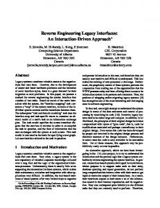
theoretical time =
(log3 n)(2+n2 ) 2000
300 250 200 150
PSfrag replacements
100 50
number of points 0 0
50
100
150
200
250
300
Figure 5: Measured and Theoretical Performance
tium III machine with 128MB of RAM, under the GNU/Linux operating system. Timings were obtained using several runs with each data set, and the results were averaged. No time variation of more than one hundredth of a second was noted for the same data set. Table 1 lists the names of the data sets, the time taken, and the number of points in the set. An indication of the symmetry determined is also given: an entry of the form (a, b, c : d) indicates that tolerances were found that created consistent groupings of a, b and c groups, and that each of these had d symmetries. An entry with one symmetry means an asymmetric object, since this one symmetry is the permutation that maps each point to itself. Sometimes many asymmetric collections were considered, but the larger part of the time was spent on the symmetric collections. In Table 1 the names of the data sets reflect the content. Penta is a pentagon, cube is a cube, cubeoct1 and cubeoct2 are variants of a cubeoctahedron, and so on. The time taken by the algorithm is considered in terms of a scatter plot of time and number of points. Since the time taken depends non-trivially on the symmetries found, the plot is not fundamentally a plot of a function. However we consider the asymptotic worst case running time in terms of the number of points. Previous analysis indicated that a function of the form (a+bnc )(logd n) would be appropriate. Informal analysis found a best fit for c ≈ 2 and d ≈ 3. The data file that does not fit this pattern is rhombix. It consists of 120 structurally equivalent points. Rhombix is unusual in that it has as many symmetries as there are points and, other than the regular prisms (which can be checked for) it has the largest number of points for which this is possible and so, as a special case it does not affect the order of the algorithm. Figure 5 shows a graph with the function (log 3 n)(2 + n2 )/2000 together with the data points listed in Table 1. Prism60 is a 60 sided prism with 180 points, prism50 is a 50 sided prism with 250 points. It is noted that these test objects
Symmetries of collections of points can be split into two categories. Firstly we have the prismatic groups comprising of some collection of rotations about a specific axis, and reflections parallel and orthogonal to this axis. Then there is a finite number of other possible collections of symmetries. A collection of points that is several times as long as it is across can only have prismatic symmetries. The result of applying the above algorithm, scanning only to a depth of four points, is that a long collection of points is seen approximately as a linear arrangement. The collection is then modified by magnifying the distance of each point radially from the central line. As this does not affect the rotational or mirror symmetries referred to that line, the radially magnified collection is then analysed for approximate symmetry in a second pass. The other collections, which have a lower aspect ratio, will be correctly analysed the first time.
7 TESTING A number of point collections derived from vertices of polyhedra were used as test cases for the algorithm. The original shapes were: pentagon, cube, cube-octahedron, icosahedron, icosidodecahedron, and rhombicosidodecahedron. The actual collections of points were obtained by combining scaled versions of the originals, and by replacing single points by one, two or three randomly translated points. Two further collections were generated as the vertices of 50- and 60-fold regular prisms, together with some extra points. Because of the relatively large number of symmetries that these objects have they are trickier to process than a typical engineering object. In practice objects which can be reverse engineered are limited in complexity, for example to no more than about 200 vertices, and so these examples cover the more difficult cases for the algorithm. The implementation of the algorithm was run on a 450Mhz Pen-
7
Development Ltd. for the model generating software. This research was funded by EPSRC grant GR/M78267.
take considerably less time in relation to the number of points than rhombix does. In particular we need to go to more than twice the number of points before we get up to the time taken by the heavily symmetric rhombix. The ability of the algorithm to find exactly the same symmetries reported by a human is very good. In all the above test cases it determined exactly those symmetries that a human found, the only issue being that some symmetries of size 1 were output, which of course is simply a case of an asymmetric object. However, as these are not impossibly numerous they can simply be eliminated from consideration afterwards, and only non-trivial symmetries can be included. Trials with many objects showed that prisms with an aspect ratio of greater than 5:1 could not typically be analysed with the algorithm as described. For example a 10:1 pencil shaped prism with 6 fold rotational symmetry was judged only to have mirror reflection about the mid point. The algorithm grouped the points at each end into a single point. The line between these two points was the symmetry axis of the collection. The case that takes the least time is that of a completely asymmetric object as there are no non-trivial matches for the registration set. Thus, after running several scans of about n steps, the algorithm will terminate upon the discovery that it can extend this to a complete match. This takes O(n log 4 n) time. The worst case for a typical engineering object is a simple prism with a large number of sides. In this case the number of registration maps is roughly equal to the number of symmetries, which is 2n. Thus the number of rotations is n/2 and the number of symmetries including reflections, is four times this. So, in this case, the total time taken is O(n2 log4 n).
REFERENCES [1] H. Alt, K. Mehlhorn, H. Wagner, E. Welzl. Congruence, Similarity, And Symmetries Of Geometric Objects. Discrete and Computational Geometry, vol. 3, pages 237–256, 1988. [2] P. Benk˝o, R. Martin, T. V´arady. Algorithms For Reverse Engineering Boundary Representation Models. To appear in Computer-Aided Design, 2001. [3] M. de Berg, M. van Kreveld, M. Overmars, O. Schwarzkopf. Computational Geometry, Algorithms And Applications, Springer, 1997. [4] J. E. Goodman, J. O’Rourke (eds.). Handbook Of Discrete And Computational Geometry, CRC Press, 1997. [5] S. Iwanowski. Testing Approximate Symmetry In The Plane Is NP-hard. Theoretical Computer Science, vol. 80, pages 227–262, 1991. [6] X. Y. Jiang, H. Bunke. A Simple And Efficient Algorithm For Determining The Symmetries Of Polyhedra. GVGIP: Graphical Models And Image Processing, 54(1):91–95, 1992. [7] F. C. Langbein, B. I. Mills, A. D. Marshall, R. R. Martin. Finding Approximate Shape Regularities In Solid Models Bounded By Simple Surfaces. These proceedings.
8 SUMMARY
[8] E. Lockwood, R. Macmillan. Geometric Symmetry, Cambridge University Press, 1978.
The concept of exact geometric symmetry is well defined, and there are a number of algorithms that will compute the symmetries of a polyhedron in time bounded by O(n log n). The exact symmetry of an object is not robust. It is typically destroyed by any errors in the data. However, in reverse engineering the notion of approximate symmetry is useful. In order to robustly compute approximate symmetry a new precise definition has been given. A given data set might not possess a unique approximate symmetry. This makes it difficult to construct an algorithm to determine it. The pragmatic problem is to determine something to compute that will suggest and validate modifications of the model so that the new model has an exact symmetry that was not previously present. The particular definition of approximate symmetry presented in this paper has been designed to be physically significant, nonarbitrary, to lead to methods for fixing the symmetry and to be fast to compute. In practice it has been shown that this algorithm runs in an acceptable time. The computation generates approximate symmetries that are not arbitrary, but rather exist or do not exist in a collection of points with good reason. Furthermore, this computation is quite robust to noise in location of the points to beyond the level at which the algorithm is required to work for the purposes envisaged in reverse engineering. Our next goal is to extend this algorithm to finding partial asymmetries, as real engineering objects typically are not completely symmetric.
[9] G. Luk´acs, R. Martin, D. Marshall. Faithful Least-Squares Fitting Of Spheres, Cylinders, Cones And Tori For Reliable Segmentation. In: H. Budkhadj, B. Neumann (eds.), Proc. 5th European Conf. Computer Vision, vol. 1, Albert-Ludwigs Universit¨at, Freiburg, Germany, pages 671–686, Springer, 1998. [10] B. I. Mills, F. C. Langbein, A. D. Marshall, R. R. Martin. Estimate Of Frequencies Of Geometric Regularities For Use In Reverse Engineering Of Simple Mechanical Components. Submitted to Computer-Aided Design, 2000. [11] K. Sugihara. An n log n Algorithm For Determining The Congruity Of Polyhedra. Journal of Computer and System Science, vol. 29, pages 36–47, 1984. [12] S. Tate. Symmetry And Shape Analysis For Assembly-Oriented CAD. PhD Thesis, Cranfield University, 2000. [13] T. V´arady, R. Martin, J. Cox. Reverse Engineering Of Geometric Models – An Introduction. Computer-Aided Design, 29(4):255–268, 1997. [14] J. Wolter, T. Woo, R. Volz. Optimal Algorithms For Symmetry Detection In Two And Three Dimensions. The Visual Computer, vol. 1, pages 37–48, 1985.
ACKNOWLEDGEMENTS
[15] D. Wood. Data Structures, Algorithms, And Performance, Addison-Wesley, 1993.
The authors wish to thank Peter Varley from Cardiff University for valuable criticism of the exposition and Tam´as V´arady from the Hungarian Academy of Sciences and CADMUS Consulting and
[16] H. Zabrodski, D. Avnir. Measuring Symmetry In Structural Chemistry. Advances in Molecular Structure Research, vol. 1, pages 1–31, 1995.
8