Jul 30, 2010 - Curry and Schoenberg [7] have introduced another basis which has a more ...... [1] D. N. Arnold, R. S. Falk, R. Winther, Finite element exterior ...
Arbitrary High-Order Spline Finite Element Solver for the Time Domain Maxwell equations Ahmed Ratnani∗
Eric Sonnendr¨ ucker†
July 30, 2010
hal-00507758, version 1 - 30 Jul 2010
Abstract In this paper, we study high order methods for solving the time domain Maxwell equations using spline finite elements on domains defined by NURBS. Convenient basis functions for the discrete exact sequence of spaces introduced by Buffa et al [4] are exhibited which provided the same discrete structure as for classical Whitney Finite Elements. An analysis of stability of the time scheme is also developed.
Keywords. Maxwell’s equations, Spline Finite Element method, Isogeometric analysis, Time domain. AMS subject classification. 65M60
1
Introduction
Since their introduction, B-splines have had a great success, thanks mainly to fast and stable algorithms developed for their use. They are used as well in industry as in academic research for interpolation, data fitting and computer aided design. Recent works by Hughes and co-authors [18, 6, 19] and the introduction of iso-geometric analysis have added yet another dimension to their use, creating an interface between simulation and numerical modeling. It seems that before the recent works of Hughes [18], the use of splines as basis functions in the finite element method was quite uncommon and essentially limited to uniform B-splines using periodic conditions, even though the web-splines developed by Hoellig and co-workers provided a strategy for dealing with boundary conditions [16, 15]. The idea of iso-geometric analysis using geometric transformations and non uniform splines or NURBS appears much simpler for most applications. Compared to traditional finite elements, the main change due to the iso-geometric analysis is undoubtedly the emergence of the k-refinement, a strategy that can increase the regularity of functions through the mesh’s interfaces, to reduce the number of degrees of freedom. Modern finite element techniques for Maxwell’s equations rely on ideas from differential geometry and more precisely on the existence of discrete spaces that provide an exact De Rham sequence. Following pioneering ideas by Bossavit [2, 3] a complete theory was successively developed [14, 1]. Buffa and co-workers [4, 5] extended iso-geometric analysis to steady-state Maxwell’s equations providing a discrete exact De Rham sequence involving discrete spaces based on B-splines. ∗
INRIA Nancy Grand Est, project-team CALVI and IRMA, UMR 7501 Universit´e de Strasbourg - CNRS IRMA, UMR 7501 Universit´e de Strasbourg - CNRS, and project-team CALVI, INRIA Nancy Grand Est, 7 rue Ren´e Descartes 67084 STRASBOURG Cedex ({ratnani, sonnen}@math.unistra.fr) †
1
hal-00507758, version 1 - 30 Jul 2010
Our aim is to use this discrete sequence for the solution of the time-dependent Maxwell equations. One important feature of geometric Finite Maxwell solvers is that one of Faraday’s or Ampere’s law hold strongly in the discrete spaces and the other one needs a Galerkin Hodge operator [3]. Hence, one of the discrete equations is completely explicit and the other one involves a mass matrix that yields a linear system to be solved at each iteration. Thanks to a property of B-spline derivatives, we were able to exhibit basis functions of the discrete spaces involved in the De Rham sequence, such that the same property holds and the discrete curl or divergence, depending on the chosen formulation, is simply an incidence matrix depending only on the connectivity of the mesh, which is thus independent of the geometric transformation. We have implemented this idea in 2D, but as it is based on a tensor product approximation, it extends straightforwardly to 3D. The outline of the paper is the following. First we recall the variational formulation of the 2D Maxwell equation, then we give the most important properties of B-splines and iso-geometric analysis. After that, we construct our exact sequence of discrete spaces as spans of well chosen basis functions on a cartesian grid and explain how to transform them on the geometric domain defined by NURBS. We can then compute the semi-discrete equations in space in a matrix formulation. We then prove a stability condition when a Leap-Frog algorithm in time is used. Finally, different test cases are performed to validate the method. High-order convergence is obtained and CFL conditions are computed for different degrees of splines.
2
Variational formulation for the 2D Maxwell equations
We consider the Maxwell equations in a subdomain Ω ⊂ R2 with a regular boundary denoted by Γ = ∂Ω. We note n, the outward unit normal vector of Ω on the�boundary Γ. We recall that ∂u � ∂y in 2D, we have two curl operators, one acting on scalars curl u = , and one acting on − ∂u ∂x � � vx ∂v x vectors v = for which curl v = ∂xy − ∂v ∂y . The divergence of a vector v is defined by vy ∂vy x div v = ∂v ∂x + ∂y . We shall also need the following function spaces � H(curl, Ω) = v ∈ (L2 (Ω))2 ; curl v ∈ L2 (Ω) and H0 (curl, Ω) = {v ∈ H(curl, Ω); v × n = 0} , � H(div, Ω) = v ∈ (L2 (Ω))2 ; div v ∈ L2 (Ω) . Notice that the space that could be called � H(curl , Ω) = u ∈ (L2 (Ω))2 ; curl u ∈ L2 (Ω) is identical to H 1 (Ω). We shall therefore stick with the more usual H 1 (Ω). Finally, we recall the Green formula we will need: Z Z Z (curl G) · F dX = G curl F dX − (G × n) · F dS , ∀ F ∈ H(curl, Ω), ∀ G ∈ H 1 (Ω), (1) Ω
Ω
Γ
and Z
Z (div F)G dX = −
Ω
Z F · (∇G) dX +
Ω
F · n G dS , ∀ F ∈ H(div, Ω), ∀ G ∈ H 1 (Ω).
(2)
Γ
In 2D domains, Maxwell’s equations can be decoupled into two systems. The first involving the (Ex , Ey , Hz ) components is called the Transverse Electric (TE) mode, and the second, involving 2
hal-00507758, version 1 - 30 Jul 2010
the (Hx , Hy , Ez ) components is called the Transverse Magnetic (TM) mode. As both mode can be discretized in the same manner, we shall only consider in the sequel the TE mode which reads ∂E − curl H = −J, (3) ∂t ∂H + curl E = 0, (4) ∂t div E = ρ, (5) � � Ex where the components are defined by E = , H = Hz . These equations need to be supEy plemented with initial and boundary conditions. We shall only consider periodic or perfectly conducting boundary conditions E × n = 0 and in a second step Silver-M¨ uller absorbing boundary conditions. In order to derive a conforming Finite Element approximation of Maxwell’s equations we first need to write an appropriate variational formulation. We would like to stay with the first order version of the system and are then naturally led to a mixed formulation involving two different functional spaces for E and H. The two options are, after multiplying both equations by a test function and integrating by parts, to use Green’s formula for either one of the two equations but not for both. The first variational formulation, in the case of perfectly conduction boundary conditions, can be derived using Green’s formula (1) in Ampere’s law (3). This yields Find (E, H) ∈ H0 (curl, Ω) × L2 (Ω) such that Z Z Z d E · ψ dX − H(curl ψ) dX = − J · ψ dX ∀ψ ∈ H0 (curl, Ω), (6) dt Ω Ω Z ZΩ d Hϕ dX + (curl E)ϕ dX = 0 ∀ϕ ∈ L2 (Ω). (7) dt Ω Ω Using the Green formula (1) in Faraday’s law (4) yields the second variational formulation Find (E, H) ∈ H(div, Ω) × H 1 (Ω) such that Z Z Z d E · ψ dX − (curl H) · ψ dX = − J · ψ dX ∀ψ ∈ H(div, Ω), (8) dt Ω Ω Ω Z Z d Hϕ dX + E · (curl ϕ) dX = 0 ∀ϕ ∈ H 1 (Ω). (9) dt Ω Ω Notice that in the first variational (6)-(7) formulation the boundary condition is taken into account in strong form by putting it into the function space where E lives. On the other hand, in the second formulation (8)-(9) the boundary condition is taken into account in a weak form.
3 3.1
Splines and B-splines functions Splines
Splines are piecewise polynomials defined on the real line. We shall require that on each compact interval, they consist of a small number of non vanishing polynomial pieces. Let T ? = {t?i , 0 6 i 6 s} be a finite strictly increasing sequence of points of R. A function S on R is a spline of order k, k > 1 with the breakpoints T ? if on each interval (t?i , t?i+1 ), it is a polynomial of degree 6 p := k − 1. On the other hand, the spline can have any regularity less than p − 1 at the breakpoints. The smoothness ri of a spline S at the breakpoint t?i is defined as follows: 3
• ri := 0 if S is discontinuous at t?i , otherwise • ri is the largest integer 0 < ri 6 k so that S has continuous derivatives of orders < ri therefore, we denote the associated spline space on an interval I = [a, b], a := t?0 , b = t?s by S?k (T ? , I) which consists of all splines S of order 6 k with breakpoints contained in T ? and of smoothness > ri at t?i . Rather than use the smoothness of the spline at breakpoints, we use the defect mi := k − ri , this is the of degrees of freedom of S at t?i . A simple computation leads to dim Sk (T ? , m, I) = Pnumber s k + i=0 mi with r := (m0 , · · · , ms ). The space Sk (T ? , m, I) is called the Schoenberg space. A simple basis of the Schoenberg space is S−j (x) =
hal-00507758, version 1 - 30 Jul 2010
Si,j (x) =
(x − a)j , j = 0, · · · , k j!
(x − t?i )j+ , j = k − mi , · · · , k − 1, i = 1, · · · , s j!
Curry and Schoenberg [7] have introduced another basis which has a more local character. Their basis are splines with the smallest possible support. They are defined by means of the divided differences and called basic splines (B-splines). For more details on this subject we refer to the books of De-Boor [8] (for computational aspect), DeVore and Lorentz [9] (for more theoretical aspects).
3.2
B-Splines
Let T = (ti )16i6N +k be a non-decreasing sequence of knots. Definition 1 (B-Spline) The i-th B-Spline of order k is defined by the recurrence relation: k−1 k Njk = wjk Njk−1 + (1 − wj+1 )Nj+1
where, wjk (x) =
x − tj tj+k−1 − tj
Nj1 (x) = χ[tj ,tj+1 [ (x)
We note some important properties of a B-splines basis: • B-splines are piecewise polynomial of degree p = k − 1 • Positivity • Compact support; the support of Njk is contained in [tj , .., tj+k ] • Partition of unity:
PN
k i=1 Ni (x)
= 1, ∀x ∈ R
• Local linear independence • If a knot t has a multiplicity m then the B-spline is C (p−m) at t For each knot vector T = (ti )16i6N +k we will associate the breakpoints sequence(t?i )16i6s . Let (Pi )16i6N ∈ Rd be a sequence of control points, forming a control polygon. 4
Definition 2 (B-Spline curve) The B-spline curve in Rd associated to T = (ti )16i6N +k and (Pi )16i6N is defined by: N X M(t) = Nik (t)Pi
hal-00507758, version 1 - 30 Jul 2010
i=1
Figure 1: (left) A B-spline curve and its control points, (right) B-splines functions used to draw the curve. N = 9, p = 2 , T = {000, 14 14 , 21 12 , 34 34 , 111}
3.3
Fundamental geometric operations
e, e After modification, we denote by N k, Te the new parameters. (Qi ) are the new control points. 3.3.1
Knot insertion
One can insert a new knot t, where tj 6 t < tj+1 . For this purpose we use the DeBoor algorithm: e =N +1 N e k=k Te = {t1 , .., tj , t, tj+1 , .., tN +k } 1 16i6j−k+1 t−ti j−k+26i6j αi = ti+k−1 −ti 0 j+16i Qi = αi Pi + (1 − αi )Pi−1 3.3.2
Order elevation
We can elevate the order of the basis, without changing the curve. Several algorithms exist for this purpose. We used the one by Huang et al. [17]. e k =k+m m e i = mi + m e = N + ms N
5
e l: Differential coefficients are defined as P i ei P l=0 l l−1 l−1 1 e e e Pi = (P i+1 − Pi ) l > 0, ti+k−1 > ti+l ti+p −ti+l 0 l > 0, ti+k−1 = ti+l Q P βi = il=1 ml , 1 6 i 6 s − 1, et αi = il=1 We present the algorithm by [17]:
k−1−l k−1+m−l , 1
6i6k−2
e j , 0 6 j 6 k − 1 et P e i ,1 6 l 6 s − 1 , k − ml 6 i 6 k − 1 1. Compute P 0 βl ej, 0 6 j 6 k − 1 e j = Qj ( k−l )P 2. Compute Q 0 0 l=1 k+m−l
hal-00507758, version 1 - 30 Jul 2010
Qj k−l ej ej 3. Compute Q βl +ml = l=1 ( k+m−l )Pβl , 1 6 l 6 s − 1 , k − ml 6 i 6 k − 1 e (k−1) e k−1 4. Compute Q βl +ml+i = Qβl +ml , 1 6 l 6 s − 1 , 1 6 i 6 m e0 5. Compute Q i Note that there exist other algorithms such those given by (see [22, 21] and others). The one given in [17] is more efficient and much more simple to implement. We can also use a more sophisticated version of this algorithm to do the insertion of new knots while elevating the degree.
3.4
Refinement strategies
Refining the grid can be done in 3 different ways. This is the most interesting aspects of B-splines basis. • using the patch parameter h, by inserting new knots. This is the h-refinement, it is the equivalent of mesh refinement of the classical finite element method. • using the degree p, by elevating the B-spline degree. This is the p-refinement, it is the equivalent of using higher finite element order in the classical FEM. • using the regularity of B-splines, by increasing / decreasing the multiplicity of inserted knots. This is the k-refinement. This new strategy does not have an equivalent in the classical FEM. J.A. Evans et al. [11] studied the k-refinement using the theory of Kolmogorov n-widths. As we will see in this article, the use of this strategy can be more efficient than the classical p-refinement, as it reduces the dimension of the basis.
3.5
Grid generation
For this purpose, we use alternatively h and p-refinement. The minimal degree of the basis functions is imposed by the domain design. When inserting knots, we can use uniformly-spaced knots or non uniformly-spaced ones.
6
hal-00507758, version 1 - 30 Jul 2010
Figure 2: First line, using h-refinement with p = 2, T = {000, 111}, T = {000, 12 , 111} and T = {000, 12 , 43 34 , 111}. Second line, using p and h-refinement with p = 3, T = {0000, 12 , 1111}, T = {0000, 12 12 , 1111} and T = {0000, 21 12 21 , 1111}
Figure 3: Grid generation. 1st line: (left) after h-refinement, N1 = 17, N2 = 5, (right) after prefinement, p1 = p2 = 3. 2nd line: (left) after h-refinement p1 = p2 = 3, (right) using unstructured mesh, p1 = p2 = 2.
7
3.6
Spline finite elements on general domains
In order to use the spline finite elements on general domains, we shall use the ideas of isogeometric analysis and consider domains defined with nurbs that can be obtained via CAD software and use these nurbs to map a rectangular domain on the physical domain. e is the parametric associated cell and such that Let Q be a cell in the physical domain. Q e Q = F (Q). let JF be the Jacobian of the transformation F , that maps any parametric domain point (ξ, η) into physical domain point (x, y). F
hal-00507758, version 1 - 30 Jul 2010
Q
K
Patch
Physical Domain
Figure 4: Mapping from the patch to the physical domain: (left) initial patch, (right) patch after h-refinement in the η direction For any function v of (x, y) we associate its representation in the parametric domain ve((ξ, η)) := v ◦ F ((ξ, η)) = v((x, y)). The basis functions Ri will not be affected by these changes, the reader can always know if the we are working in the physical or parametric domain thanks to (x, y) = F (ξ, η), x = α(ξ, η) and y = β(ξ, η). then, α1 =
∂α ∂ξ
α2 =
∂α ∂η
β1 =
∂β ∂ξ
β2 =
∂β , ∂η
we have for the determinant of the Jacobian det(JF ) = α1 β2 − α2 β1 and for JF −1 � � � � 1 α1 α2 β2 −α2 JF = JF −1 = . β1 β2 ∆ −β1 α1 Let u be a (scalar or vector) function defined on the physical domain. When we use the patch coordinates, we will write it u e, idem for the used spaces.
3.7
Boundary conditions
The boundary conditions are very easy to handle. Thanks to the mapping, the boundary of the physical domain is mapped into the boundary of the patch. therefore, it becomes to treat periodic condition, by using periodic splines with an adapted knot vector [8]. The perfect conductor and Silver-Muller conditions are also simple to implement. 8
4
Construction of the finite element spaces
An important feature of the functional spaces we chose for the variational formulation is that they form an exact sequence. Depending of the variational formulation we choose, we need to work with different exact sequences. In the case of (6)-(7), the following function spaces are involved H 1 (Ω) ∪ V
grad curl −→ H(curl, Ω) −→ ∪ −→ Wcurl −→
L2 (Ω) ∪ X
(10)
In the case of (8)-(9), the following function spaces are involved H 1 (Ω)
hal-00507758, version 1 - 30 Jul 2010
∪ V
curl div −→ H(div, Ω) −→ L2 (Ω) ∪ ∪ −→ Wdiv −→ X
(11)
In order to keep the specific features of Maxwell’s equations at the discrete level we need to construct finite dimensional subspaces endowed with the same structure. The involved discrete spaces are denoted by X ⊂ H 1 (Ω), Wcurl ⊂ H(curl , Ω), Wdiv ⊂ H(div, Ω) and V ⊂ L2 (Ω). When discretizing the first variational formulation (6)-(7), we shall look for (Eh , Hh ) ∈ Wcurl × V and when discretizing the second variational formulation (8)-(9), we shall look for (Eh , Hh ) ∈ Wdiv × X.
4.1
Spline finite elements on patch grids
We shall now start constructing the actual subspaces X ⊂ H 1 (Ω), Wcurl ⊂ H(curl, Ω), Wdiv ⊂ H(div, Ω) and V ⊂ L2 (Ω). Our discrete space will be constructed using B-splines. The key point of our method is the use of the recursion formula for the derivatives: ! p−1 Ni+1 (t) Nip−1 (t) p0 Ni (t) = p − . (12) ti+p − ti ti+p+1 − ti+1 N p−1 (t)
i It will be convenient to introduce the notation Dip = p ti+p −ti . Then the recursion formula for derivative simply becomes 0 p (t). (13) Nip (t) = Dip (t) − Di+1
Discrete vector fields on a rectangular domain. Let us first consider a rectangular domain Ω. We consider the following discrete functional spaces V = span{Nip (x)Njp (y), 1 ≤ i ≤ Nx , 1 ≤ j ≤ Ny }, �� p � � � � Ni (x)Djp (y) 0 Wdiv = span , , 1 ≤ i ≤ Nx , 1 ≤ j ≤ Ny } , Dip (x)Njp (y) 0 �� p � � � � Di (x)Njp (y) 0 Wcurl = span , , 1 ≤ i ≤ Nx , 1 ≤ j ≤ Ny } , Nip (x)Djp (y) 0 X = span{Dip (x)Djp (y), 1 ≤ i ≤ Nx , 1 ≤ j ≤ Ny }. As proved in the article by Buffa et al, [4] these spaces verify the same exact property as the spaces they approximate. 9
Vector field transformations. Let us now define coordinate changes conserving either the curl or the divergence of a vector field. Let us start from a vector field Ψ(ξ, η) = (Ψ(1) (ξ, η), Ψ(2) (ξ, η))T defined on the parametric ˜ domain Q. Using the transformation formula (18) for the vector fields of Wdiv which conserves the di1 vergence, using the diffeomorphism G = F −1 , we get Ψ(1) = ∆ (α2 Ψ(2) + α1 Ψ(1) ) and Ψ(2) = 1 (2) + β Ψ(1) ) . 1 ∆ (β2 Ψ fdiv . So let Ψ = (Ψ(1) , Ψ(2) )T be a function in Wdiv , and Ψ = (Ψ(1) , Ψ(2) )T be a function in W fdiv on the physical domain is To save the divergence property, the corresponding space of W Wdiv = {Ψ := (
1 1 (α1 Ψ(1) + α2 Ψ(2) ), (β1 Ψ(1) + β2 Ψ(2) ))T , ∆ ∆
fdiv } Ψ∈W
therefore, �
hal-00507758, version 1 - 30 Jul 2010
Wdiv = span
4.2
� � � �� 1 ep e p (η) α1 , 1 D e p (ξ)N e p (η) α2 Ni (ξ)D . j j β1 β2 ∆ ∆ i
The Discrete Equations
Let us now express the equation satisfied by the approximations Eh , Hh when using each of the variational formulations we introduced. Let’s start with (8)-(9). In this case we look for Eh ∈ Wdiv and Hh ∈ H 1 (Ω). We first notice that due to the exact sequence property we have divEh ∈ X. Let us denote by � p � � � 0 Ni (x)Djp−1 (y) 1 2 ψ i,j = , ψ i,j = Dip−1 (x)Njp (y) 0 we have � Wdiv = span ψ 1i,j , ψ 2i,j ,
1 ≤ i ≤ Nx , 1 ≤ j ≤ Ny } ,
Denoting the components of Eh by (Ehx , Ehy ), we have Ehx (t, x, y)
=
Ny Nx X X
exi,j (t)Nip (x)Djp (y),
Ehy (t, x, y)
=
Ny Nx X X
eyi,j (t)Dip (x)Njp (y),
i=1 j=1
i=1 j=1
and Hhz (t, x, y)
=
Ny Nx X X
hzi,j (t)Nip (x)Njp (y).
i=1 j=1
Using these expansions on the finite element bases, we can compute explicitly, for curl Hh =
Ny Nx X X
0
hzi,j (t)
i=1 j=1
Nip (x)Njp (y) 0 −Nip (x)Njp (y)
!
we now use the formula (12), curl Hh =
Ny Nx X X
hzi,j (t)
i=1 j=1
=
Ny Nx X X
p−1 Nip (x)(Djp−1 (y) − Dj+1 (y)) p−1 p−1 −(Di (x) − Di+1 (x))Njp (y)
!
hzi,j (t){ψ 1i,j − ψ 1i,j+1 − ψ 2i,j + ψ 2i+1,j }
i=1 j=1
10
We will use the following convention: for a knot vector T = (ti )16i6N +k generating the ”N ” B-splines of order k, {Nik , 1 6 i 6 N }, we put Njk := 0 for any j > N . By making a change of index in the sum, we get curl Hh =
Ny Nx X X
hzi,j {ψ 1i,j
−
ψ 2i,j }
−
i=1 j=1
y +1 Nx NX X
i=1 j=2
hzi,j−1 ψ 1i,j
+
Ny NX x +1 X
hzi−1,j ψ 2i,j
i=2 j=1
therefore, curl Hh =
Ny Nx X X
(hzi,j − hzi,j−1 )ψ 1i,j − (hzi,j − hzi−1,j )ψ 2i,j
i=2 j=2
+
Ny Nx X X {hz1,j − hz1,j−1 }ψ 11,j + {hzi−1,1 − hzi,1 }ψ 2i,1 + hz1,1 ψ 11,1 − hz1,1 ψ 21,1
hal-00507758, version 1 - 30 Jul 2010
j=2
i=2
in case of periodic boundary conditions, we get a strong form of the discrete Ampere’s law (8) which can be written −1 j, (14) −e˙ + Rhz = MW where hz , ex , ey the vectors of spline coefficients, MW is the mass matrix for Wdiv and R consists of two blocks of the discrete derivatives in the x and y directions of these vectors. Remark We’ve shown that we can write K T = MW R, where K is the matrix involved in the classical formulation (without courant field) : � MW e˙ = Kh MV h˙ = −K T e A discrete Faraday’s law can be obtained from the variational formulation (7) which can be written h˙ z + dx ey − dy ex = 0, (15) where dx and dy the discrete derivatives in the x and y directions. We have thus obtained matrix differential equations on the vectors of spline coefficients that can be solved by any appropriate ODE solver. For example, for a second order time discretization, a leap-frog or Verlet scheme is well adapted.
4.3
Solving strategy
The use of Isogeometric analysis for solving the Maxwell’s equations is not immediate. The problem is the De Rham diagram that requires certain regularity of the domain which is logic. Let us illustrate our purpose. (1) (2) Let Tp , Tp , 1 6 i, j 6 N + p + 1 be two open vectors knots, where we choose N1 = N2 = N and p1 = p2 = p for simplicity. To get the discrete De Rham diagram, the discrete spaces involved in our scheme must be: p,p Sα,α (P) ⊂ H 1 (Ω),
p,p−1 p−1,p Sα,α−1 × Sα−1,α (P) ⊂ H(div, Ω)
where α = {−1, m, · · · , p − m, −1} is the smoothness of the Spline space at the breakpoints, i.e each interior knot has a multiplicity m. 11
Let us assume that the domain, using appropriate control points, is generated by the knots vectors (1) (2) Tp−1 , Tp−1 . If we denote by m the multiplicity of interior knots, we see that after the elevation (1)
(2)
degree process, we will have the vectors Tp , Tp with a multiplicity m + 1 of the interiors knots. therefore, some parts ( at the interior knots ) of our domain must be of a regularity p − m. This can be done by suppressing the redundant knot. Remark, that when using NURBS this is a more difficult process. We now present the strategy for solving Maxwell’s equation using B-splines: • we model exactly our domain, using NURBS, B-splines or any other mapping, which can maps the physical domain into a rectangular domain ”patch”, • if the domain can not be exactly represented, we can interpolate, or approximate the physical domain using B-splines or NURBS, [20, 13],
hal-00507758, version 1 - 30 Jul 2010
• the discrete spaces are generated by B-splines such they can respect the exact discrete De Rham sequence.
5
Leap Frog scheme’s stability
In this section we will give a preview of the time discretization scheme we used to solve the linear system obtained and some classical results. Let us first, just recall the general formulation of the LF scheme. For the linear system � MW e˙ = Kh MV h˙ = −K T e the LF time discretization of order N is given by ( 1 n+1 n MW E ∆t−E = KN H n+ 2 3
MV
1
H n+ 2 −H n+ 2 ∆t
T E n+1 = −KN
where � KN
KN = K ,N = 2 −1 T −1 ∆t2 = K(I − 24 MW KMV K ) , N = 4 1
1
We define the global energy by E n := 12 {(E n )T MW E n + (H n− 2 )T MV H n+ 2 } We have the following lemma: Lemma 1 The global energy is stationary, i.e E n+1 = E n 1
Proof Let us put E n+ 2 =
E n+1 +E n . 2
Then we have,
1 3 1 1 1 1 E n+1 − E n = ((E n+1 )T MW E n+1 + (H n+ 2 )T MV H n+ 2 − ((E n )T MW E n − (H n− 2 )T MV H n+ 2 ) 2 2 1 1 3 1 1 n+1 T n+ 12 n T = (E ) MW E − (E ) MW E n+ 2 + (H n− 2 )T MV (H n+ 2 − H n+ 2 ) 2 1 1 3 1 1 = (E n+ 2 )T MW (E n+1 − E n ) + (H n− 2 )T MV (H n+ 2 − H n+ 2 ) 2
using the time discretization scheme, we have: 1
1
1
1
E n+1 − E n = ∆t(E n+ 2 )T KN H n+ 2 − ∆t(H n+ 2 )T KN E n+ 2 12
Therefore, we have E n+1 − E n = 0 The stability of the scheme depends on the global energy, it must be a positive quadratic form Lemma 2 E n is a positive quadratic form if ∆t 6
2 dN ,
−1
−1
T M 2k where dN = kMV 2 KN W
hal-00507758, version 1 - 30 Jul 2010
Proof 1 1 1 1 1 1 1 ∆t n− 1 T E n = (E n )T MW E n + (H n− 2 )T MV H n+ 2 = (E n )T MW E n + (H n− 2 )T MV H n− 2 − (H 2 ) MV E n 2 2 2 2 1 1 1 1 1 1 1 ∆ −1 −1 2 2 > kMW k2 + kMV2 k2 − |(H n− 2 )T MV2 MV 2 T KN MW 2 MW En| 2 2 2 1 1 1 1 1 1 1 ∆dN 2 2 {kMV2 H n− 2 k2 + kMW > kMW k2 + kMV2 k2 − E n k2 } 2 2 2 1 1 1 1 1 1 ∆dN 1 2 2 k2 + kMV2 k2 − Enk > kMW kMV2 H n− 2 kkMW 2 2 4 1 1 1 ∆tdN 2 > (1 − k2 + kMV2 k2 } ){kMW 2 2 N The last quantity is positive if 1 > ∆td 2 . 2 th th Finally, we can take CF LN = hdN . As proved in [12], we have CF Lth 4 ' 2.85CF L2 .
6
Numerical results
The theoretical convergence rate is ”p + 1” for the magnetic field H z and ”p” for the electrical field E, where p = min(p1 , p2 ).
6.1
Test case 1: square
The analytical solution in this case is: H z = cos(k1 x + φ1 ) cos(k2 y + φ2 ) cos(ωt) k2 E x = − cos(k1 x + φ1 ) sin(k2 y + φ2 ) sin(ωt) ω k2 y E = sin(k1 x + φ1 ) cos(k2 y + φ2 ) sin(ωt) ω For our test we took a computational domain of size [0, 2π] × [0, 2π] and k1 = k2 = 1,
φ1 = φ2 = 0,
ω=π
This test enables to check the L2 norm of the error (in log scale) between the numerical and e analytical solution, with respect to the parameter h = max{diam(Q)}, for different orders of the basis functions (from order 3 to order 6). This is shown in figure 5. We verify that the slopes of the different curves correspond to the order of the basis functions. In particular, for high orders, the machine precision is achieved. For validation, we solved the Maxwell’s equation for 1 1 1 1 N = 16, 32, 64, 128, with dt = 100 , 200 , 400 , 800 . The L2 error is then computed after respectively 5, 10, 20, 40 iterations so as to keep the same final time. Thanks to the regularity of the basis functions, we see that we can achieve a good precision with a lower number of meshes. In other words, the k-refinement strategy helped as to reduce 13
hal-00507758, version 1 - 30 Jul 2010
Figure 5: Square test: the L2 norm error for (left) the magnetic field , (right) the electric field
Figure 6: Square test: (left) the dimension of the discrete spaces Wh and Vh , (right) the L2 norm error for the electric field, where the vector knots are multiplicity m = 1, 2 for quadratic B-splines
the number of degrees of freedom as we can see it in the figure 6, where the number of degrees of freedom was reduced by a factor of 6. The price to pay, is that we increased the support of the basis functions compared to the classical finite element method. But as we said before, this is the best we can do using splines functions, the B-splines have the minimal support that we can get if we try to increase the regularity of our basis. Tables (1,2) show the CFL numbers for different B-splines degree p = 2, · · · , 5. We see that the CFL decreases with the B-splines degree and the knots multiplicity.
6.2
Test case 2: circular wave guide
The analytical solution, in the polar coordinates, in this case is:
14
p p p p
= = = =
2 3 4 5
LF 2T h 0.3044 0.2058 0.1496 0.1151
LF 2num 0.3056 0.1840 0.1520 0.1168
LF 4T h 0.8676 0.5866 0.4265 0.3281
LF 4num 0.8720 0.5872 0.4272 0.3280
Table 1: Test case 1: CFL numbers (theoretic and numerical values), for splines of degree p = 2, · · · , 5
hal-00507758, version 1 - 30 Jul 2010
p p p p
= = = =
2 3 4 5
m=1 0.8720 0.5872 0.4272 0.3280
m=2 0.5200 0.4224 0.3056 0.2304
Table 2: Test case 1: CFL, using LF4, for splines of degee p = 2, · · · , 5 for singular knots (m = 1), and doubled knots (m = 2)
H z (r, θ) = − cos(ωt + θ){J1 (ωr) + aY1 (ωr)} E θ (r, θ) =
1 sin(ωt + θ){J0 (ωr) − J2 (ωr) + a(Y0 (ωr) − Y2 (ωr))} 2 1 E r (r, θ) = − cos(ωt + θ){J1 (ωr) + aY1 (ωr)} ωr
where Jn , Yn are the first and the second Bessel functions of order n. For our test we took rmin = 0.65138750344695903414,
rmax = 0.99000418530735846839,
a = 1.0,
ω = 3π
We used uniform periodic B-splines in the theta direction and uniform B-splines with open knots in the radial direction. The use of uniform B-splines allows as to reduce the number of degrees of freedom. therefore, we can achieve an error of 10−11 , using quintic B-splines, with only 64 × 64 meshes, and dim Wh = 8640, dim Vh = 4352. A precision of 10−7 is achieved, using quintic B-splines, with only 16 × 16 meshes.
6.3
Test case 3: Silver-Muller condition
In the case of the Silver-Muller condition the discrete Faraday’s equation of (9) is written ∂t MV hz + Ke + Γhz = 0 where R Γ is the mass matrix of the discrete Vh on the boundary that checks Silver-Muller condition i.e ∂ΩSM Ni,j Ni0 ,j 0 In this test we see the evolution of an electromagnetic wave (figure 6.3 ), under Silver-Muller condition on both the internal and external boundary. At t = 0 we took Ex = u(x)u(y)0 and 2 EY = u(x)0 u(y), with u(x) = exp(− (x−m) ). 2σ 2 15
hal-00507758, version 1 - 30 Jul 2010
Figure 7: Circular wave guide test: (left) at t = 0, (right) after 20 iterations, for N = 64, p = 3
7
Conclusions and perspectives
We presented a new scheme for Maxwell’s equation using B-splines functions, which enables as to reduce the number of degrees of freedom thanks to the k-refinement. Our method can be easy used with an integrated CAD system. However, the use of the Isogeometric idea requires to verify the De Rham diagram, so, we can not always use an exact modeling. therefore, we will need to approximate or interpolate domains using either splines or NURBS functions. Another idea, which can be a great help is the use of GB-Splines. GB-Splines are a general basic splines, and verify a closed relation to (12): G0i,k (t) = with
Gi,k−1 (t) Gi+1,k−1 (t) − , ci,k−1 ci+1,k−1
(n−2) ψi,n (t), (n−2) Gi,2 (t) = φ (t), i+1,n 0,
k>3
t?i 6 t 6 t?i+1 t?i+1 6 t 6 t?i+2 t∈ / (t?i , t?i+2 )
R t? (n−2) (n−2) and ci,k−1 = t?i+k−1 Gi,k−1 (t)dt, ψi,n , φi,n are assumed to be strictly monotone on (t?i , t?i+1 ) i and (t?i+1 , t?i+2 ) respectively. We can get the classical polynomial spline of order n by taking φi,n (t) = −
(t − t?i )n−1 , (n − 1)!hi
ψi,n (t) =
16
(t − t?i )n−1 , (n − 1)!hi
hi = t?i+1 − t?i
hal-00507758, version 1 - 30 Jul 2010
Figure 8: Circular wave guide test: the L2 norm error for, first line E x (left) and E y (right) components of the electric field, second line the magnetic field
17
hal-00507758, version 1 - 30 Jul 2010
Figure 9: Evolution of an electromagnetic wave in circular domain under Silver-Muller boundary condition
18
A
Transformation compatible with grad, div and curl operators
hal-00507758, version 1 - 30 Jul 2010
In order to define our basis functions on the parametric domain, which is a rectangular domain of R2 with cartesian coordinates and then to map them onto a patch of the physical domain, we need to define a transformation of scalar and vector fields which is compatible with our differential operators (grad, div and curl). This is provided to us by the pullback operator for differential forms which is designed to commute with the exterior derivative. Hence compatible transformations will be provided to us by associating our scalar or vector fields to a well chosen differential form and using the pullback. In our case, we have differential forms defined on Q and need to construct the associated differential forms on K. For this we need a C 1 diffeomorphism G : K → Q. Let us recall the pullback formula for 0, 1 and 2-forms. A 0-form on Q is a function (or a scalar field) ϕ(ξ, η). The pullback of ϕ on K is in this case simply ϕ = ϕ ◦ G. A 1-form on the parametric space can be written ω = ω 1 (ξ, η)dξ + ω 2 (ξ, η)dη. Denoting by G1 and G2 the components of the diffeomorphism G, the pullback of ω on K is then defined by ω = G∗ ω = ω 1 ◦ G dG1 + ω 2 ◦ G dG2 � � � � ∂G2 ∂G1 ∂G2 ∂G1 + ω2 dx + ω1 + ω2 dy, = ω1 ∂x ∂x ∂y ∂y
(16)
where we denote by ω1 (x, y) = ω 1 ◦ G(x, y) and ω2 (x, y) = ω 2 ◦ G(x, y). A 2-form on the parametric space can be written σ(ξ, η) dξ ∧ dη and its pullback on K by the diffeomorphism G is defined by σ(x, y) dx ∧ dy = G∗ (σ dξ ∧ dη) = σ ◦ G dG1 ∧ dG2 � � ∂G1 ∂G2 ∂G2 ∂G1 − dx ∧ dy, = σ(x, y) ∂x ∂y ∂x ∂y
(17)
where we denote by σ(x, y) = σ ◦ G(x, y). Now a vector field in a 2D space is associated to a differential 1-form. This 1-form depends on the sequence of spaces we are working on and is chosen such that its exterior derivative corresponds either to the curl or the divergence of the vector field. Note that in both cases a function ϕ (or scalar field) can be associated to either a 0-form which is the function itself or the two form ϕ dξ ∧ dη. Let us start with the case of (10). In this case the exterior derivative of a 0-form should be associated to the grad operator and the exterior derivative of a 1-form should be associated to the curl operator. This is the case if we associate a generic vector field Ψ(ξ, η) = (Ψ(1) (ξ, η), Ψ(2) (ξ, η))T to the differential form ω c = Ψ(1) (ξ, η) dξ + Ψ(2) (ξ, η) dη. Indeed, take a function (or 0-form) ϕ. Then, on the one hand gradϕ = (∂ξ ϕ, ∂η ϕ)T which is associated to the one form ∂ξ ϕ dξ + ∂η ϕ dη = dϕ, an on the other hand curl Ψ(ξ, η) dξ ∧ dη = (∂ξ Ψ(2) − ∂η Ψ(1) ) dξ ∧ dη = dω c . 19
Let us now consider the case of (11). Then the exterior derivative of a 0-form should be associated to the curl operator and the exterior derivative of a 1-form should be associated to the div operator. This is the case if we associate a generic vector field Ψ(ξ, η) = (Ψ(1) (ξ, η), Ψ(2) (ξ, η))T to the differential form ω d = Ψ(1) (ξ, η) dη − Ψ(2) (ξ, η) dξ. Indeed, take a function (or 0-form) ϕ. Then, on the one hand curl ϕ = (∂η ϕ, −∂ξ ϕ)T which is associated to the one form ∂η ϕ dη − (−∂ξ ϕ dξ) = dϕ, an on the other hand
hal-00507758, version 1 - 30 Jul 2010
div Ψ(ξ, η) dξ ∧ dη = (∂ξ Ψ(1) + ∂η Ψ(2) ) dξ ∧ dη = dω d . Having now associated our functions and vector fields to differential forms, we can use the expression of the pullbacks to define the adequate scalar and vector field transformations. In particular, when using the spaces associated to (11). We need to transform the basis functions associated to V , this is straightforward as they are functions associated to 0-forms, and to Wdiv . To defined the transformation of a vector field Ψ(ξ, η) = (Ψ(1) (ξ, η), Ψ(2) (ξ, η))T ∈ Wdiv we use the pullback formula (16) for the1-form ω d = Ψ(1) (ξ, η) dη − Ψ(2) (ξ, η) dξ. This yields � � � � ∂G1 ∂G2 ∂G1 ∂G2 (2) (1) (2) (1) +Ψ ◦G dx + −Ψ ◦ G +Ψ ◦G dy, ωd = −Ψ ◦ G ∂x ∂x ∂y ∂y which is associated to the vector field � � ∂G1 ∂G2 ∂G1 ∂G2 T (2) (1) (2) (1) Ψ = (−Ψ ◦ G +Ψ ◦G ), (Ψ ◦ G −Ψ ◦G ) . ∂y ∂y ∂x ∂x
(18)
References [1] D. N. Arnold, R. S. Falk, R. Winther, Finite element exterior calculus, homological techniques, and applications. Acta Numer. 15 (2006), pp 1–155. [2] A. Bossavit, Mixed finite elements and the complex of Whitney forms, The Mathematics of Finite Elements and Applications VI, J. Whiteman (ed.), 137–144, Academic Press, London, 1988. [3] A. Bossavit, Computational electromagnetism and geometry. (5): The ’Galerkin hodge’ , J. Japan Soc. Appl. Electromagn. & Mech., 8, 2 (2000), pp. 203–209. [4] A. Buffa, G. Sangalli, R. Vazquez, Isogeometric analysis in electromagnetics: B-splines approximation, Comput. Methods Appl. Mech. Engrg. 199, pp. 1143–1152, (2009). ´ zquez, Isogeometric Analysis in Electromagnetics: theory and testing. [5] A. Buffa, J. Rivas, G. Sangalli, R. Va Preprint. [6] J.A Cottrell, T. Hughes, Y. Bazilevs, Isogeometric Analysis, toward Integration of CAD and FEA, first ed., John Wiley & Sons, Ltd, (2009). [7] H.B. Curry, I.J. Schoenberg On Polya frequency functions IV: The fundamental spline functions and their limits, J. d’Analyse Math. 17, 71-107; Ch. 5:137, 141 (1966).
20
[8] C. De Boor, A practical guide to splines, Springer-Verlag, Berlin, Heidelberg, vol 27 (2001). [9] R.A. DeVore, G.G. Lorentz, Constructive Approximation, Springer-Verlag, Berlin, Heidelberg, (1993). ¨ rfel, B. Ju ¨ ttler, B. Simeon, Adaptive isogeometric analysis by local h-refinement with T-splines, [10] M.R. Do Comput. Methods Appl. Mech. Engrg. 199, pp. 264–275, (2010). [11] J.A. Evans, Y. Bazilevs, I. Babuska, T. Hughes, n-Widths, supinfs, and optimality ratios for the k-version of the isogeometric finite element method, Comput. Methods Appl. Mech. Engrg. 198, pp. 1726–1741, (2009). [12] H. Fahs, S. Lanteri, A high-order non-conforming discontinuous Galerkin method for time-domain electromagnetics, J. Comput. Appl. Math., Vol. 234, pp. 1088-1096 (2010). [13] W. Heidrich, R. Bartels, G. Labahn, Fitting Uncertain Data with NURBS, in Proc. 3rd Int. Conf. on Curves and Surfaces in Geometric Design, Vanderbilt University Press, (1996). [14] R. Hiptmair, Finite elements in computational electromagnetism, Acta Numerica 11, pp. 237–339, (2002).
hal-00507758, version 1 - 30 Jul 2010
¨ llig, Finite Element Methods with B-Splines. Frontiers in Applied Mathematics 26, SIAM, 2003. [15] K. Ho ¨ llig, U.Reif, J.Wipper, WeightedextendedB-splineapproximationofDirichlet problems. SIAM J. Numer. [16] K.Ho Anal. 39-2, pp. 442–462 (2001). [17] Q.X. Huang, S.M. Hua, R.R. Martin, Fast degree elevation and knot insertion for B-spline curves, Comput. Aided Geom. Design 22, pp. 183–197, (2005). [18] T. Hughes, J. A. Cottrell, Y. Bazilevs, Analysis: CAD, finite elements, NURBS, exact geometry and mesh refinement, Comput. Methods Appl. Mech. Engrg. 194, pp. 4135-4195, (2005). [19] T. Hughes, A. Reali, G. Sangalli, Efficient quadrature for NURBS-based isogeometric analysis, Comput. Methods Appl. Mech. Engrg. 199, pp. 301–313, (2010). [20] W. Ma, J.P. Kruth, NURBS Curve and Surface Fitting for Reverse Engineering, Int. J. Adv. Manuf. Technol. 14, pp. 918–927, (1998). [21] L. Piegl, W. Tiller, The NURBS Book, second ed., Springer-Verlag, Berlin, Heidelberg, (1995). [22] H. Prautzsch, B. Piper, A fast algorithm to raise the degree of B-spline curves, Computer Aided Geometric Design 4, pp. 253–266, (1991). [23] T.W. Sederberg, D.L. Cardon, J. Zheng, T. Lyche, T-spline Simplification and Local Refinement, ACM Trans, Graphics 23 (3) pp. 276–283, (2004).
21