netic interactions in unbounded domains. ... tions of frequency-domain finite methods beyond the ... complexity and available computer resources dictate. The.
Frequency-Domain Finite Element Methods for Electromagnetic Field Simulation: Fundamentals, State of the Art, and Applications to EMI/EMC Analysis Andreas C. Cangellaris Center for Electronic PackagingResearch,ECE Department University of Arizona, Tucson, AZ 85721,U.S.A. ature has been generated on the application of the finite scattering and radiation problems. The book by J.M. Jin [l] serves both as a tutorial on the procedures for the application of the finite element method to the approximation and solution of electromagnetic boundary value problems, and as a rather thorough survey of the classesof problems that have been tackled. Considering the power of the aforementioned attributes, one would have expected that the method of finite elements would have gained in popularity among EMC/EMI engineers and would have established itself as the method of choice in the analysis and predicplex geometries are examined. Such domain decom- tion of EM1 and the design of electromagnetically compatposition techniques are expected to play an important ible systems. Nevertheless, a literature review indicates role in the continuing effort to extend the applicathat this is not the case. As an example we mention that tions of frequency-domain finite methods beyond the in a special issue of the IEEE Transactions on Electromagsubcomponent-level to component and system modelnetic Compatibility, dedicated to computational methods ing for electromagnetic interference and electromagfor EMI/EMC analysis, very few papers on finite elements netic compatibility analysis and design. appeared, and the applications presented where limited to rather simple problems of low complexity [2]-[3]. Before one attempts to search for drawbacks in the I. INTRODUCTION method of finite elements that have prevented its proliferThere are two attributes of the method of finite ele- ation as an EMI/EMC prediction tool, one has to keep in ments that have prompted the rapid growth of its appli- mind that application of electromagnetic CAD for compocation to the modeling of electromagnetic interactions in nent and system EMI/EMC is actually still at its infancy. electronic systems. One of them is its superior modeling The reason for this is that the complexity of an integrated versatility where structures of arbitrary shape and compo- electronic component, subsystem or system is such that sition can be modelled as precisely as the desirable model accurate modeling of source, coupling mechanism, and recomplexity and available computer resources dictate. The ceiver of electroma.gneticnoise is almost prohibitive using second, is common to all differential equation-based nu- a single numerical method for solving Maxwell’s equamerical methods, and has to do with the fact that the tions, irrespective of the type of the method used. More matrix resulting from the discretization of the governing specifically, considering the tremendous variation in feaequations is very sparse, which implies savings in com- ture size from chip, to package, to board, to cables, to puter memory for its storage as well as in CPU time for shields, it becomes clear that the number of elements reits inversion. Clearly, these two attributes come at the quired for the discretization of such a system for finite expense of an increase in the degrees of freedom used in element analysis of electromagnetic interactions is out of the numerical approximation of the problem since now, the reach of today’s most powerful supercomputers. contrary to integral equation methods, the entire space In view of the above and recognizing that an elecsurrounding all sources of electromagnetic fields needs be tromagnetic analysis tool will be useful as a CAD tool incorporated in the numerical model. Nevertheless, be- only if simulation times are in the order of minutes or cause of the sparsity of the resulting matrix and the sim- at most a few hours, this paper examines the latest adplicity with which complex geometries can be modeled, vances in the method of finite elements that are expected this increase in the degreesof freedom of the approxima- to help the method establish itself as a reliable candidate tion is an acceptable penalty. for EMI/EMC problem solving either at the component level or in conjunction with reduced-order electromagnetic Over the past ten years, a significant volume of liter107 O-7803-3207-5/96/$5,00 0 1996lEEE
Abstract-This paper provides a critical review of frequecy-domain finite element methods and their applications to the modeling of electromagnetic interactions in complex electronic components and systems. Emphasis is placed on latest advances in finite element grid generation practices, element interpolation function selection, and robust, highly absorbing numerical grid truncation techniques for modeling electromagnetic interactions in unbounded domains. These advances have helped enhance the robustness and accuracy of the method. Finally, the advantages of domain decomposition techniques for the modeling of com-
element method to a variety of electromagnetic
models of subsystems. As a matter of fact, it is this area where the method of finite elements can have an important impact. Indeed, current practices of EMI/EMC analysis concentrate on rather simplistic, individual source-tovictim models, which often suffer from their inability to capture the impact of surrounding conducting, dielectric, and magnetic material topology on the electromagnetic interaction. The finite element method allows for the development of a more precise model that will lead to higher accuracy in noise prediction and thus facilitate the design of electromagnetically compatible electronic modules. Finally, the potential of domain decomposition methods for reducing the complexity of the original problem will be examined. The basic idea behind such methods is the partitioning of the domain of interest into smaller ones and the development of the solution in a piecewise manner, one subdomain at a time, using different types of both numerical and analytic techniques. The inherent parallelism of such approaches combined with the smaller size of the subdomains makes them extremely well-suited for massively-parallel computation. II. MATHEMATICAL FRAMEWORK FOR FINITE ELEMENT ANALYSIS The focus of this paper is on the numerical approximations of Maxwell’s equations with time-harmonic field variation. Therefore, the following discussion pertains to linear sources and materials. However, time-domain finite methods that can handle transient electromagnetic interactions in the presence of nonlinear sources and nonlinear media are possible and are currently the topic of vigorous research within the computational electromagnetics community. As a matter of fact, the finite-element formulation in [2] is such that both transient and time-harmonic electromagnetic simulations can be effected within a single mathematical framework. In order to review the basic steps involved in the finite element approximation of electromagnetic boundaryvalue problems, let us consider the double-curl equation for the electric field, E, which, in a source-free, isotropic and linear medium with position-dependent magnetic and electric properties has the form Vx
(&VxE)+jwiE=O,
The time dependence exp(jwt) is assumed (j = G), and the complex permittivity, E = c - ja/w, is used to account for any conduction and/or dielectric losses in the medium. For the purposes of finite element solutions, a weak form of (1) is required. For node baaed finite element expansions the unknown vector field is approximated in terms
of scalar basis functions, &,
E=CEidi,
(2)
where Ei denotes the unknown vector field value at node i. The relevant weak form, in the spirit of Galerkin’s approximation, is
((
&V
X E) x V&) -
1 -ii f jwp
+ (j&E&)
=
x (V x E)gS&
(3)
where ( ) and $ indicate integration over the domain of interest and its boundary, respectively, while ii is the outward unit normal on the boundary. For edge element expansions, vector basis functions, Ni, are used for the expansion of the field, E = C EiNiy where Ei are the unknown coefficients in the expansion. The relevant weak form is
((
LO X E) * (V X Ni)) 3WP 1 -G -f jwp
+ (j&E
* Ni)
=
X (V X E) . Nids
(5)
For two-dimensional problems, a scalar version of (3) is readily obtained. More specifically, for a transverse magnetic to z (TM,) polarization, the fields, E = bE, H = kH, + 9Hy, are independent of z and (3) reduces to
(C
&Vx,,>
. Vxyh)
+ (jwtEq$)
=
(6. VE)(bjdZ (6) f ‘jwp
where VW = S/&Z + ?a/ay. For transverse electric to z (TE,) polarization of the two-dimensional fields, where H = i?H, E = S?, + QE,, the weak form is easily found from (6) by duality. For static problems (w = 0), a scalar potential, @, is often introduced, and the electric or magnetic fields are obtained in terms of the gradient of the potential. For such cases, it is a weak statement of Laplace’s equation for the scalar potential that is being derived. The most well-known attribute of Galerkin’s method, where the solution is sought in a finite-dimensional subspace of the class of admissible functions for the problem of interest using the same set of functions as trial and test functions, is the symmetry of the resulting stiffness matrix given a symmetric weak formulation. However, another important merit of Galerkin’s method is that, if a symmetric weak formulation is used, Galerkin’s approximate 108
solution exactly conserves energy in the electromagnetic field despite the fact that it satisfies the vector Helmholtz equation only approximately over the domain of interest. This is easily shown starting from (5) and using the complex conjugate of the field, E*, as the test function and Faraday’s law to introduce the magnetic field in the boundary integral
((
$V
x E) . (V x E’)) + (jw?E . E*) = f
(fi x H) . E”ds
(7)
The complex conjugation of (7), use of Faraday’s law to simplify the integrand in the first term on the left, and use of the constitutive relations B = pH, D = 1E, result in the following equation (-jwB
. H’) + (jwD* . E) =
f
(E x H*) . iids
(8)
Clearly, the resulting expression is Poynting’s theorem for time-harmonic fields. Thus energy conservation in the electromagnetic field is satisfied exactly by the approximate solution. The importance of the aforementioned result is rather significant. Considering the various potential sources of error in the development of a numerical solution to a boundary value problem, it is definitely advantageous to be able to work with a weak statement that is consistent with the correct physics of the field we are attempting to calculate. For the electromagnetic field problems of interest, the calculated field quantities will be acceptable only if they satisfy both energy conservation and electric charge conservation. As a matter of fact, the latter has been found to be extremely important in the finite element solution of three-dimensional vector electromagnetic problems. In later sections, it is pointed out that modifications to the weak statement in (3) and careful selection of the vector basis functions in (5) are needed to prevent the contamination of the numerical solution from spurious fields caused by the lack of enforcement of charge conservation in the original weak statement. In order to illustrate the development of the numerical approximation of the electromagnetic boundary value problem, let us consider the weak statement in (5). Substitution of (4) into (5) and testing with each and every one of the vector basis functions N.J results in a linear system of simultaneous equations
while the elements of the forcing vector are &G
.fj=-f
X (V X E) * Njds
01)
M is the number of degrees of freedom in the approximation. One of the important attributes of the method of finite elements is that that the basis functions used have local support, i.e. they are non-zero only over a set of adjacent elements. This is what leads to the sparsity of the resulting system since most of the elements Aij are zero. The forcing vector is formed by contributions of the surface integrals over the domain boundaries. From the uniqueness theorem, the tangential component of the magnetic field, -(l/jwp)G x (V x E), on the domain boundaries is all that is needed for a unique solution of Maxwell’s equations inside the domain. This tangential magnetic field on the domain boundary is used to account for all sources exterior to the domain of interest. The surface term in (5) is used also for enforcing tangential magnetic field continuity conditions at material interfaces. As far as tangential electric field boundary conditions are concerned, they are taken into account in the construction of the basis functions. This is discussed in more detail in Section 4. III.
GRID GENERATION
Numerical grid generation is probably the most critical step in a finite element analysis of electromagnetic wave interactions. During the early stages of the application of the finite element method to modeling of electromagnetic interactions, the emphasis was on mathematical model and weak statement formulations and their subsequent use in the analysis of propagation, radiation and scattering problems in conjunction with rather simple geometries. Consequently, the important issue of automatic generation of finite element grids appropriate for electromagnetic propagation and scattering problems received rather limited attention. Apparently, the assumption was that grid generation practices used in low-frequency electromagnetic field modeling and/or other areas of engineeering in which the method of finite elements was already being used, could be adopted without significant alteratioEs. This turned out to be a rather false assumption, simply because the specific physics of the phenomenon that is being analyzed needs be taken into account before a discrete model is built for its quantification. The famous sampling iheorem of modern communication theM ory for the sampling of a band-limited signal serves as a AijEi=fj, j=l,Z&...,M c simple, yet powerful example. id Extensive research over the past few years has led to where the elements, Aij, of the so-called stiffness matrix the understanding and quantification of the impact of the are given by discrete approximations of wave equations on the accuracy and quality of the simulated wave solutions [5]-[8]. -VxNi).(VxNj))+(jv’Ni.Nj)(lO) The findings from such analysis are now being used as 109 I
guidelines and/or constraints in the development of procedures for automatic grid generation. The following is a list of undebatable results that are used to guide the construction of a finite element grid for the modeling of electromagnetic wave propagation, radiation and scattering problems.
new solution is then attempted with the refined grid, and the process is repeated until the desirable solution accuracy has been achieved. While the manipulation of hexahedral meshes, i.e., meshes that use the so-called brick elements, is much simpler than that of a tetrahedral mesh, tetrahedral meshes First and foremost, the grid must provide for adequate are the ones that have been adopted for automatic grid wavelength resolution in order to minimize numerical dis- generation. (In two dimensions, brick elements reduce to persion (i.e., artificial, discretization induced dependence quadrilaterals while tetrahedra reduce to triangles.) The of phase velocity on electrical grid size) and thus con- reason for this is that triangles and tetrahedra are simtrol phase error. The number of degrees of freedom per plices in two and three dimensions, respectively. Comwavelength, required to achieve a fixed accuracy, is de- plete polynomial expansion functions are defined easily on simplex elements. Furthermore, an arbitrary domain, pendent on the degree of the interpolating polynomials used in the, constyruction of the basis functions, the elec- no matter how complicated it might be, can always be discretized automatically into a set of simplex elements using trical size of the domain (i.e., the size of the domain in Delaunay tesselation [9]. As a matter of fact, grid generwavelengths), and the boundary conditions used for grid ation software baaed on the Delaunay algorithm and its truncation. Furthermore, problem geometry and matevariants is now commercially available and is being used rial properties impact the way the finite element grid is for finite element grid generation with fairly satisfactory constructed. Electromagnetic fields exhibit singular beresults. Consequently, most of the recent advances on auhavior at material wedges and corners (especially metaltomatic mesh generation and mesh refinement are based lic), which cannot be resolved properly by the polynomial on Delaunay triangulation. interpolating functions used for the finite element approximation. Thus, grid refinement or use of special elements With regards to automatic mesh generation, new proare required in the vicinity of such geometric features to cedures have been developed for preventing the occurence improve solution accuracy. In addition, abrupt changes of degenerate (sliver) elements, for the redistribution of in the electric permittivity and the magnetic permeabilexisting nodes and/or the efficient incorporation of new ity of materials need be accompanied by appropriate grid nodes for improving the quality of the tetrahedra (i.e. size changes in order to both prevent the occurrence of making them as equilateral as possible), and for preserv(nonphysical) numerical reflections and maintain the con- ing prescribed material boundaries during the process of ditioning of the finite element matrix. Finally, the grid initial mesh generation as well as during subsequent mesh generation process should be such that element degen- refinement [lO],[ll]. eracy (i.e. triangles degenerating toward line segments, As far as mesh refinement is concerned, a variety of quadrilaterals approaching triangles, or tetrahedrons de- procedures are currently available. At this point, it is imgenerating to quadrilaterals) never occurs. Such elements portant to point out that in addition to the so-called h lead to ill-conditioning and may eventually render the firefinement, where new nodes are introduced in the grid nite element solution useless. while the order of the polynomial approximation remains While it is often tempting to adopt the philosophy that the same, solution accuracy can be improved by increasing the finer the grid the better the quality of the solution, the order of the polynomial interpolation while keeping one needs to remember that an excessively fine mesh (un- the number of nodes the same. This so called p refinement less needed) wastes computational resources and thus it tends to be less popular than h refinement, mainly due to should be avoided. Consequently, it is important that the the desire of maintaining low interpolation function comgrid generation process is such that adaptive mesh refine- plexity within regions of high material complexity. Howment is possible. In other words, for the purposes of com- ever, one should keep in mind that h refinement cannot be putation efficiency, the analysis begins with the construcpushed to arbitrarily small element sizes. The reason for tion of an initial mesh the density of which has been de- this is that as the mesh is progressively refined the eigencided on the basis a specific set of constraints perinent to value spectrum of the stiffness matrix widens; hence the the material properties, the characteristics of the sources system becomes progressively more ill-conditioned [12]. and anticipated spatial variation of the electromagnetic This progressive ill-conditioning of the stiffness matrix as the mesh is refined results in an increase in the roundfields. A simulation is attempted using this mesh. Next, an error estimator is used to examine the quality of the off error which counteracts the decrease in approximation solution over the entire grid and thus identify areas where error. At some point, approximation error and round-off mesh refinement is needed to improve solution accuracy. error become equal, and any further mesh refinement will result, in deterioration in the accuracy of the solution. As Such mesh refinement is then effected using appropriate pointed out in [12], the round-off error does not depend mesh refinement schemes that maintain element quality and preserve mesh conformity to material boundaries. A strongly on the degree of the interpolating polynomials. 110
It depends mainly on element size, h, and, for the secondorder problems of interest in electromagnetic modeling, the dependence is of the form O(he2). Consequently, the way to maintain accuracy and postpone the deleterious effect of round-off is to increase the order of the interpolating polynomials (p refinement). The numerical experiments in [13] support this conjecture in a very illustrative manner. We conclude this section by pointing out that before adaptive mesh refinement can be effected, a reliable a posterioti error estimate to be used as a refinement criterion is required. A variety of error estimators have been proposed over the past few years [14]-[171. As expected, they depend on the physical attributes of the fields as well as the choice of functions and interpolating elements used in the finite element approximation. IV. THE CHOICE OF ELEMENTS Most of the original applications of the finite element method to vectorial electromagnetic field modeling in three dimensions were based on the so-called nodal elements, using field representations of the form shown in (2) and weak statements such as the one in (3). In other words, the degrees of freedom were defined to be the three components of the unknown fiield quantity at the element nodes. It was soon found that such approximations were plagued by the occurrence of non-physical, spurious modes [18]. These spurious solutions manifested themselves as modes with nonzero divergence, and were caused by the inability of the aforementioned choice of interpolation and weak statement to enforce Gauss’ law for divergence-free solutions. Consequently, a variety of approaches were proposed for eliminating these spurious modes within the context of nodal elements [19]-[21]. A different approach to eliminating spurious modes that has gained popularity over the past few years is the use of the so-called edge elements [22]. Edge elements use vector basis functions of the form shown in (4). They have the unique property that the degrees of freedom associated with these elements are the circulations of the vector field along the edges of the mesh. The important implication of this fact is that edge elements impose the continuity of only the tangential components of the unknown electric (or magnetic) field across element boundaries, which is obviously consistent with the physical constraints for electromagnetic field solution uniqueness inside a domain. Additional advantages of edge elements are: a) Boundary conditions at material interfaces are automatically enforced through the natural boundary condition in the weak statement (see the surface integral term in (5)). b) Dirichlet boundary conditions are easily imposed along element edges. This second property becomes extremely useful when dealing with conducting boundaries, especially those that exhibit wedges and cor-
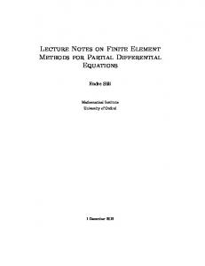
k Fig. 1. Whitney l-form edge element.
ners. The most popular version of these edge elements is the so-called Whitney l-form. It was long before the method of finite elements was becoming a popular tool in boundary value problem solving that Whitney described a family of polynomial forms on a simplicial mesh with special properties that made them attractive for electromagnetic field representations [23]. These polynomials are of, at most, degree one on tetrahedra. Any two p-forms are said to conform on a surface if they take the same values at any given set of p vectors tangent to the surface. Finally, p-forms are uniquely determined by integrals on p-simplices. Let us consider, for example, the popular Whitney l-forms (Fig. 1). They are associated with mesh edges. Each edge in the tetrahedral mesh contributes an independent basis function. In other words, the degrees of freedom of the approximation are associated with the element edges; this is the reason they are called “edge elements.” For an edge e = {i, j} connecting vertices i and j the basis function is given by Ne = We =