Figure 1(b) illustrates some derivatives estimated using the .... Arnoldi's method is found in Krylov subspace methods for spectral analysis and ... where p is a trial step, g = âf is the gradient of the objective, and W = â2f is the Hessian, or an .... The reduced gradient, VT g, is the directional derivative of the objective in the ...
AIAA 2015-2943 AIAA Aviation 22-26 June 2015, Dallas, TX 16th AIAA/ISSMO Multidisciplinary Analysis and Optimization Conference
Arnoldi-based Sampling for High-dimensional Optimization using Imperfect Data Jason E. Hicken∗ and Anthony Ashley†
Downloaded by Jason Hicken on July 27, 2015 | http://arc.aiaa.org | DOI: 10.2514/6.2015-2943
Rensselaer Polytechnic Institute, Troy, New York, 12180
We present a sampling strategy suitable for optimization problems characterized by high-dimensional design spaces and noisy outputs. Such outputs can arise, for example, in time-averaged objectives that depend on chaotic states. The proposed sampling method is based on a generalization of Arnoldi’s method used in Krylov iterative methods. We show that Arnoldi-based sampling can effectively estimate the dominant eigenvalues of the underlying Hessian, even in the presence of inaccurate gradients. This spectral information can be used to build a low-rank approximation of the Hessian in a quadratic model of the objective. We also investigate two variants of the linear term in the quadratic model: one based on step averaging and one based on directional derivatives. The resulting quadratic models are used in a trust-region optimization framework called the Stochastic Arnoldi’s Method (SAM). Numerical experiments highlight the potential of SAM relative to conventional derivative-based and derivative-free methods when the design space is high-dimensional and noisy.
I.
Introduction
Large-scale numerical simulations play a central role in contemporary aircraft design, and, increasingly, this role goes beyond the use of simulations as proxies for experiments. This trend is exemplified by differential-equation-constrained optimization (DECO), which couples simulations with numerical optimization. DECO has been used to optimize highly-refined aircraft where small improvements translate into significant economic and environmental benefitsa . Moreover, DECO has the potential to enable the design of unprecedented aircraft configurations where empirical data is sparse and intuition is lacking. Clearly, DECO has enormous value and potential for aerospace engineers; however, while DECO algorithms for steady and periodic deterministic systems are maturing, there remains a broad class of problems that cannot be optimized with conventional algorithms. These problems exhibit 1. a high-dimensional design space, 2. complex physics that must be modeled using large-scale simulations, and 3. simulation outputs, e.g. lift force or total energy, that are “imperfect”. In this context, imperfect outputs are quantities of interest whose numerical errors cannot be eliminated, at least in practice; consequently, such outputs fail to meet the underlying assumptions of conventional gradient-based optimization algorithms. The word imperfect is intentionally chosen to distinguish these errors from more traditional numerical errors that can, usually, be estimated and effectively reduced. In the following sections, we briefly elaborate on two such sources of imperfect data. ∗ Assistant
Professor, Department of Mechanical, Aerospace, and Nuclear Engineering, Member AIAA Student, Department of Mechanical, Aerospace, and Nuclear Engineering, Student Member AIAA a For example, a 1% reduction in the fuel consumed by the worldwide fleet would result in 7 million fewer tonnes of C02 emitted per year [1]. † Graduate
1 of 15 American Institute of Aeronautics and Astronautics Copyright © 2015 by Jason E. Hicken and Anthony Ashley. Published by the American Institute of Aeronautics and Astronautics, Inc., with permission.
90 final states
85
50
objective function approx. derivative
80
40
75 30 20
z
JT
10
two initial conditions 20
10
x
0
−10
−20 20
10
0
−10
70 65 60 55
0 −20
50
y
45 30
32
34
(a)
36
ρ
38
40
42
44
(b)
Downloaded by Jason Hicken on July 27, 2015 | http://arc.aiaa.org | DOI: 10.2514/6.2015-2943
Figure 1. Example trajectories of the Lorenz DE (left) illustrating sensitive dependence on initial conditions. A time-averaged objective (right) exhibits high-frequency fluctuations; moreover, only approximate derivatives can by computed, in this case using an ensemble adjoint.
A.
Time-averaged Outputs from Chaotic Systems
The outputs of interest in many engineering systems are time-averages of chaotic solutions. Relevant examples include the lift and drag on aerodynamic bodies [2], the energy produced by a fusion reactor [3], and the (phase-averaged) pressure in an internal-combustion engine [4]. Chaotic systems are characterized by a sensitive dependence on initial conditions; the distance between two states that are “close” initially will exponentially increase with time. This is illustrated in Figure 1(a) using the Lorenz DE [5] and two initial conditions that satisfy k∆x0 k ≤ 10−10 . In addition to the initial conditions, chaotic systems are sensitive to other parameters. This has significant implications for time-averaged outputs, which we illustrate using the Lorenz system and the objective function Z T 1 2 (z(t, ρ) − ztarg ) dt, JT (ρ) = 2T 0 where z(t, ρ) is one of the Lorenz state variables, ztarg = 35, and T > 0 is the period of integration. The design variable here is ρ, a parameter in the Lorenz DE. Figure 1(b) plots the Lorenz objective JT versus the parameter ρ for an averaging period of T = 400. High-frequency oscillations can be observed in the objective function JT . In theory, we could eliminate these fluctuations by integrating over an infinite time horizon, but, in practice, we must truncate the simulation at a finite T . The oscillations in JT reflect the sensitivity of the Lorenz DE to changes in ρ, and they hint at the difficulties of using gradient-based optimization. Indeed, as T → ∞ the gradient of JT diverges [6] despite the fact that the objective itself converges. Researchers have proposed methods to compute derivatives of objectives that depend on chaotic systems, such as the ensemble adjoint [6–8] and least-squares adjoint [9]. These methods share one shortcoming: they produce estimates of the derivatives only. Figure 1(b) illustrates some derivatives estimated using the ensemble adjoint. Although the derivatives capture the general slope of the objective, errors are clearly visible. Such errors are incompatible with conventional gradient-based optimization. B.
Uncertainty Propagation in High-dimensional Input Spaces
Numerical simulations contain many sources of uncertainty. For example, turbulence and combustion models introduce errors with respect to the true physics, the operating conditions of a system are not deterministic (e.g. the Reynolds number is not known precisely), and perturbations to the intended design are introduced by the manufacturing process. The field of optimization under uncertainty (OUU), a branch of uncertainty quantification (UQ), seeks to account for such uncertainties during the optimization process. OUU can help ensure good performance over a range of parameters, and it can help reduce the probability of failure. Typically, at each iteration of an OUU, uncertainties in the input parameters must be propagated through the numerical simulation to deduce uncertainties in the outputs, e.g. the standard deviation in a force or 2 of 15 American Institute of Aeronautics and Astronautics
1.5 1.0
100
dominate 1D subspace based on eigenvalues of ∇2 f at (−0.5, 0)
0.5
y¯
80
E[f ]
0.0
−0.5
correctly accounting for subspace changes
90
PDFs of the random variables
−1.0 −2.0 −1.5 −1.0 −0.5
0.0
0.5
1.0
70 60
1.5
x¯
50 −0.10
(a)
assuming subspace is fixed: 12% error in derivative −0.05
0.00
0.05
distance along slice in Fig. a
0.10
(b)
Downloaded by Jason Hicken on July 27, 2015 | http://arc.aiaa.org | DOI: 10.2514/6.2015-2943
Figure 2. Uncertainty propagation can be made tractable for large numbers of (aleatory) inputs by identifying dominant subspaces using, e.g., the Hessian (left). However, accurately differentiating such dimensionreduction strategies is usually not practical, and errors are inevitable (right).
energy. Uncertainty propagation is especially challenging when there are a large (> 100) number of uncertain input parameters. These situations require approximations to cope with the “curse of dimensionality”. Several parameter-selection and model-reduction strategies have been proposed for the propagation of stochastic, or aleatory, uncertainties in high-dimensional input spaces [10–12]. Methods of propagating epistemic uncertainties, i.e. model errors, in high-dimensional spaces have also been investigated [13, 14]. If these methods are to be used for high-dimensional OUU problems, derivative information will be needed; however, differentiating these propagation methods accurately is not practical. Therefore, an optimization algorithm must account for the discrepancy between the outputs and their derivatives. To illustrate why dimension-reduction strategies are difficult to differentiate, consider computing the expected value, E[f (x)], of the Rosenbrock function � �2 2 f (x + ξ) = [1 − (x + ξ)] + 100 (y − η) − (x + ξ)2 , where x = (x, y)T ∈ R2 are the design variables and ξ, η ∈ N (0, 0.52 ) are Gaussian random variables. In this example, we use the dominant eigenvalue of the Hessian to define a subspace for dimension reduction. Figure 2(a) shows one such subspace defined at x = (−0.5, 0)T . Figure 2(b) plots the expected value obtained by (correctly) accounting for changes in the subspace. The figure also plots the expected value obtained by fixing the subspace, which reflects how derivatives would be computed for most dimension-reduction strategies. Fixing the subspace results in a 12% error in the derivative. Note that, to correctly compute the derivative in the present example, we would need to differentiate eigenvectors of the Hessian, which would be impractical for high-dimensional outputs based on simulations. C.
Other Sources of “Imperfect” Outputs
Time-averaging in chaotic systems and uncertainty propagation in high-dimensional spaces are two important examples that produce imperfect data and motivate the current work. However, inconsistencies between the outputs and their derivatives can also arise in other applications of DECO. 1. Cut-cell [15–17] and immersed-boundary methods [18–20] are popular and effective methods for numerically solving DEs on complex, moving geometries. In geometry optimization, these methods produce discontinuities in the design space as the mesh-topology and/or stencil is updated. A similar problem exists when unstructured grids are regenerated during shape optimization. 2. The differentiate-then-discretize [21], or “continuous” [22], adjoint yields derivatives that are inconsistent with the discretized output. See, for example, [23, 24]. 3. Incomplete sensitivities have been proposed [25, 26] to reduce the computational cost of computing the gradient. The terms that are dropped or estimated in these approaches necessarily result in approximate derivatives. 3 of 15 American Institute of Aeronautics and Astronautics
4. A multi-fidelity approach may be used in which a higher fidelity tool produces the output but a lower fidelity method is used to estimate gradients [27]. The inaccuracies 1 and 2 described above are discretization errors that can be reduced through mesh refinement. However, the mesh refinement needed to sufficiently reduce these errors may not be possible in practice, and in these cases the algorithms proposed below could be helpful.
Downloaded by Jason Hicken on July 27, 2015 | http://arc.aiaa.org | DOI: 10.2514/6.2015-2943
D.
Imperfect Data and the State-of-the-art
The examples above highlight important emerging applications — high-dimensional uncertainty propagation and simulation of chaotic systems — in which outputs of interest and their derivatives exhibit some form of inaccuracy. If we want to optimize these outputs, can we rely on state-of-the-art optimization methods? For low-dimensional design spaces, derivative-free optimization methods could be effective for the applications described above. These methods include deterministic interpolation/regression-based surrogate models [28–30], the Nelder-Mead simplex method [31], and genetic algorithms [32,33]. However, “it is usually not reasonable to try and optimize problems with more than a few tens of variables...” with derivative-free methods [30]. Derivative-based algorithms are highly scalable, making them ideally suited for optimization of smooth functions in large design spaces. Although the challenge of differentiating the simulation software is a potential drawback, algorithmic-differentiation [34] has made this task easier. Unfortunately, derivativebased algorithms are also not suitable for the target applications, because they require sufficient accuracy in the data and consistency between the outputs and their derivatives. Stochastic approximation (SA) algorithms [35–38] can be used to optimize functions whose evaluation contains noise. Some forms of SA also permit the use of noisy gradients [35, 39]. There are both theoretical and practical issues with applying SA to the applications described earlier. Theoretically, the “noise” must be unbiased and independent of the design space [38], and these assumptions are not met by the target applications. From a practical perspective, SA algorithms tend to use many “low quality” iterations to ensure (probabilistic) convergence, so function and gradient evaluations must be inexpensive. This requirement is also not fulfilled by the DE-constrained optimization problems under consideration. Reduced-order models (ROM) offer a distinct approach from derivative-free and derivative-based optimization. Rather than tackling the DE-based optimization directly, ROM methods first seek a simplified, and presumably less expensive, model for the DE simulation. Subsequently, the optimization is performed using the ROM as a surrogate for the full DE model. Methods in this class include projection-based approaches like proper-orthogonal decomposition [40–44]. These approaches typically fix the design parameters while constructing the ROM, although a method that accounts for parameter dependence was recently proposed by Lieberman et al. [45] in the case of steady, linear DEs. However, building parametric ROMs for nonlinear and/or unsteady DEs remains an active and challenging area of research.
II.
Arnoldi Sampling
The primary contribution of this work is a sampling procedure that is suitable for high-dimensional input spaces when the gradient is available, but potentially inaccurate. The sampling procedure is based on Arnoldi’s method, which we briefly review below. A.
Arnoldi’s Method
Arnoldi’s method is found in Krylov subspace methods for spectral analysis and solving linear systems; see, for example, [47] and [48] and the references therein. In those applications, Arnoldi’s method is used to construct an orthogonal basis for the Krylov subspace Km (A, z) ≡ span{z, Az, A2 z, · · · , Am−1 z}, where A is a square matrix and z is a vector. A version of Arnoldi’s method based on modified Gram-Schmidt is provided in Algorithm 1 for reference. An important feature of Arnoldi’s method is that A is not required explicitly: only matrix-vector products of the form Azj are needed. We exploit this aspect of the algorithm in the proposed sampling procedure. To understand the origins of the proposed sampling procedure, it is helpful to review how Arnoldi’s method is traditionally used in the context of optimization. Efficient optimization algorithms for C 2 objectives apply Newton’s method, or a quasi-Newton method, to the first-order optimality conditions. For
4 of 15 American Institute of Aeronautics and Astronautics
Algorithm 1: Arnoldi’s method. Data: z1 ∈ Rn such that kz1 k = 1 Result: Z = [z1 , z2 , . . . , zm+1 ], an orthonormal basis for Km+1 (A, z1 ) 1 2 3 4 5 6 7 8 9 10
for j = 1, 2, . . . , m do zj+1 = Azj for i = 1, . . . , j do (Modified Gram-Schmidt) T hi,j = zj+1 zj zj+1 ← zj+1 − hi,j zj end compute hj+1,j = kzj+1 k if khj+1,j k = 0 then return (check for breakdown) zj+1 ← zj+1 /hj+1,j end
Downloaded by Jason Hicken on July 27, 2015 | http://arc.aiaa.org | DOI: 10.2514/6.2015-2943
unconstrained convex problems, Newton’s method produces systems of the form Wp = −g, where p is a trial step, g = ∇f is the gradient of the objective, and W = ∇2 f is the Hessian, or an approximation to it. When Algorithm 1 is used in this setting, A becomes W and Arnoldi’s method reduces to the symmetric Lanczos algorithm that appears in the conjugate gradient method. Thus, when applied to optimization problems, Arnoldi’s method requires Hessian-vector products. These products can be computed in several ways, including algorithmic differentiation [34] and, when PDEs are involved, second-order adjoints [49–51]. The products can also be computed using a finite-difference approximation applied to the gradient, since � B.
� g(x + �zj ) − g(x) ∇2 f zj = lim . �→0 �
Arnoldi Sampling
Arnoldi’s method can be transformed into a sampling procedure by recognizing that the Hessian-vector products selected by the algorithm represent infinitesimal samples. If these infinitesimal perturbations are made finite, they can be used as a sampling procedure. In other words, the sample locations are defined by xj = x0 + αzj , where α > 0 is the sample radius, and the zj are defined by Arnoldi’s method with Azj replaced with [g(x0 + αzj ) − g(x0 )] /α. This Arnoldi sampling procedure is listed in Algorithm 2. In addition to providing the sample locations and sampled data, Algorithm 2 also produces approximations to the eigenvalues and eigenvectors of the Hessian; see lines 16 and 17. This approximation is based on iterative eigenvalue methods [47, 52]. The eigen-decomposition in Arnoldi sampling uses the symmetric part of Hm , the m×m upper Hessenberg matrix composed of the hi,j . In contrast, the conventional Arnoldi’s method for spectral analysis uses the matrix Hm itself. We use the symmetric part, because Hm reduces to a symmetric matrix when the gradients are accurate and α → 0. This also avoids the generation of a complex spectrum, which would not be appropriate in the context of a Hessian. When the gradients are accurate and α is chosen suitably, Arnoldi sampling reduces to a Arnoldi’s method with finite-difference approximations for the Hessian-vector products. Like finite-difference approximations, α must be chosen carefully to achieve optimal performance. Unlike finite-difference approximations, our proposed method benefits from a relatively large sampling radius, one that would normally cause undesirable truncation errors in a finite-difference approximation. C.
Eigenvalue Accuracy Study
We use the dominant eigenvalues produced by the Arnoldi sampling procedure to build a quadratic model for optimization; therefore, it is important to verify and quantify the accuracy of the approximate eigenvalues. 5 of 15 American Institute of Aeronautics and Astronautics
Algorithm 2: Arnoldi sampling. Data: m > 0, α > 0, x0 , f0 = f (x0 ) and g0 = g(x0 ) Result: sampled locations Xm+1 = [x0 , x1 , x2 , . . . , xm ] sampled function values Fm+1 = [f0 , f1 , . . . , fm ] sampled gradient values Gm+1 = [g0 , g1 , . . . , gm ] approximate eigenvalues, Λm = [λ1 , λ2 , . . . , λm ], and approximate eigenvectors of the Hessian Vm = [v1 , v2 , . . . , vm ] 1 2 3 4 5 6 7 8
Downloaded by Jason Hicken on July 27, 2015 | http://arc.aiaa.org | DOI: 10.2514/6.2015-2943
9 10 11 12 13 14 15 16 17
set z1 = −g0 /kg0 k for j = 1, 2, . . . , m do set xj = x0 + αzj sample fj = f (xj ) and gj = g(xj ) compute zj+1 = (gj − g0 )/α for i = 1, . . . , j do (Modified Gram-Schmidt) T hi,j = zj+1 zj zj+1 ← zj+1 − hi,j zj end compute hj+1,j = kzj+1 k if khj+1,j k = 0 then (check for breakdown) set m = j and break end zj+1 ← zj+1 /hj+1,j end � 1� ˜m = V ˜ m Λm . compute eigen-decomposition of the symmetric part of Hm , i.e. Hm + HTm V 2 ˜m compute the approximate eigenvectors Vm = Zm V
To this end, we apply Algorithm 2 to a set of quadratic objectives with different eigenvalue distributions. In particular, the objective is defined by F (x) = xT EΣET x, (1) where E denotes the 2p ×2p orthonormalized Hadamard matrix, whose columns are the synthetic eigenvectors. p p The diagonal matrix Σ ∈ R2 ×2 holds the synthetic eigenvalues, given by Σi,i =
1 , iq
where q = 21 , 1, or 2. For this investigation, we consider n = 256 variables. We run Arnoldi sampling with m = 16 iterations and a sample radius of α = 1. The initial point about which samples are taken is (x0 )i = sin(i), i = 1, 2, . . . , 256. Noise with a Gaussian distribution is added to each component of the gradient. The noise has mean zero and its standard deviation is either 0.5%, 2.5% or 5%, relative to the norm of the initial gradient at x0 . Figure 3 shows the relative error in the first 8 estimated inverse eigenvalues: ˜ −1 ˜ −1 −1 errori = λ − λ /λ = / λ − 1 λ , i i i i i ˜ i is the ith estimated eigenvalue and λi is the exact eigenvalue. Recall that the eigenvalue distributions where λ √ 256 2 256 are given by {1/ i}256 i=1 , {1/i}i=1 , and {1/i }i=1 ; the results for the three distributions are plotted left to right in the figure. The blue dot in the figures denotes the median value of the error over 100 runs, and the lower and upper bars represent the 0.025 and 0.975 probability quantiles, respectively. The magnitude of the noise increases from 0.5% in the top set of figures to 5% in the bottom set of figures. For reference, the red squares denote the error in the estimated eigenvalues when no noise is present. Overall, the plots suggest that the dominant eigenvalues estimated by Arnoldi sampling are resilient over a range of noise magnitudes. In addition, the results indicate that spectra whose energy decays quickly are less affected by noise; nevertheless, it is important to point out that relative errors in eigenvalues with small magnitude can have a pronounced impact on the optimization steps. 6 of 15 American Institute of Aeronautics and Astronautics
Downloaded by Jason Hicken on July 27, 2015 | http://arc.aiaa.org | DOI: 10.2514/6.2015-2943
(a) 0.5% noise
(b) 2.5% noise
(c) 5% noise
Figure 3. Relative accuracy in the inverse of the eigenvalues approximated using Arnoldi sampling with varying noise magnitude.
7 of 15 American Institute of Aeronautics and Astronautics
(a) accurate gradient
(b) inaccurate gradient
Downloaded by Jason Hicken on July 27, 2015 | http://arc.aiaa.org | DOI: 10.2514/6.2015-2943
Figure 4. Even when the Hessian is exact, a small error in the gradient can significantly impact the quality of the step.
The results in Figure 3 also suggest that Arnoldi sampling should not be used with relative noise above 5%; however, this conclusion pertains to the chosen radius of α = 1 only, since an increase in α tends to reduce the impact of noise. On the other hand, an increase in α risks an increase in truncation error for strongly nonlinear functions.
III.
Stochastic Arnoldi’s Method
In this section, we describe how Arnoldi sampling can be used in an optimization framework. The key idea is to form a quadratic model based on the estimated eigenvalues and eigenvectors, and seek a candidate step p in the span of the eigenvectors: 1 q(p) ≡ f¯ + g¯T p + pT VΛVT p, 2 p∈span(V) min
subject to
kpk ≤ ∆,
(2)
where the diagonal matrix Λ ∈ Rr×r holds the r < m largest (in magnitude) eigenvalue estimates from Arnoldi sampling, and V ∈ Rn×r are the corresponding eigenvector estimates. Note that (2) includes a trust-radius constraint, with radius ∆ > 0, to handle the possibility of nonconvex models. We have not yet specified how f¯ and g¯ are estimated in the trust-region subproblem (2). While the function value has no influence on the solution of p, it does play a role in the step-acceptance procedure described later. The linear term g¯, on the other hand, does impact p. A na¨ıve choice would be to set g¯ = ∇f (x0 ), i.e. the gradient evaluated at the initial pointb . Although this is a natural choice for accurate data, it can lead to inaccurate steps in the presence of errors, even if the Hessian model is exact; this is illustrated in Figure 4. In the following subsections, we propose two possible choices for g¯ that attempt to ameliorate errors in the gradient. A.
Variant 1: Step Average
We can view each of the points xj , j = 0, 1, . . . , m, produced by Arnoldi sampling as a potential location at which to center the quadratic model. For each of these locations, we can adopt the corresponding gradient, gj , in the model q(p) and find a step. Let pj = Vyj denote this step. Substituting this step into (2), and ignoring the trust-radius constraint for the moment, the solution is pj = −VΛ−1 VT gj . The trial solution for point j is xj + pj . Averaging over all potential trial solutions, we obtain m
xnew =
1 X (xj + pj ) = x ¯ − VΛ−1 VT g¯, m + 1 j=0
P P where x ¯ = ( j xj )/(m + 1) and g¯ = ( j gj )/(m + 1). In the sequel, we will refer to this as the step-average approach. Note that, if the trust-radius constraint is present, we solve (2) with g¯ defined as the average gradient. b The
initial point for Arnoldi sampling is the current iterate of the outer optimization loop.
8 of 15 American Institute of Aeronautics and Astronautics
B.
Variant 2: Directional Derivatives
Downloaded by Jason Hicken on July 27, 2015 | http://arc.aiaa.org | DOI: 10.2514/6.2015-2943
Our numerical experiments suggest that step averaging is effective when the error has mean zero; however, it does not address bias in the error. This is not surprising, because g¯ is a simple average, so the bias will persist. As an aside, we remark that constant bias in the set {gj }m j=0 does not impact the eigenvalue and eigenvector approximation in Arnoldi sampling, because these approximations are based on differences in the gradient. To address bias in the construction of g¯, we examine the form of the (unconstrained) solution when the step is in the subspace V and g¯ is the exact gradient: � p = Vy, where y = Λ−1 −VT g . We see that the reduced-space solution, y, is the inverse of Λ acting on the reduced-space negative gradient. This is an important observation, because it means we can focus on approximating VT g rather than g. The reduced gradient, VT g, is the directional derivative of the objective in the estimated eigenvector directions, V. These directional derivatives can be approximating using the sampled function values: f1 − f0 f2 − f0 1 ˜T T ˜T V VT g = V Z g ≈ g ≡ red . 1:m,1:r m , α 1:m,1:r .. fr − f0 where gred denotes the approximate reduced gradient. By using the function values to approximate the directional derivatives, we eliminate bias in the gradient error. When the trust-region constraint is present, the reduced-space solution is found by solving the trustregion problem (2) with g¯ = Vgred , and adding the step, p = Vy, to the point x0 as defined in Arnoldi sampling. We will refer to this as the directional-derivative variant. C.
Comparison of the Two Variants
We use the synthetic quadratic objective, defined earlier by (1), to study and compare the two proposed variants for g¯. As before, we use n = 256 variables and set α = 1. The initial point provided to the Arnoldi sampling algorithm is (x0 )i = sin(i), i = 1, . . . , 256. The Hessian model is constructed using the r = 4 largest estimated eigenvalues and eigenvectors from Arnoldi sampling, which is run with m = 16 iterations. We consider two models for error. The first model adds Gaussian noise with mean zero to the function, F , and its gradient, ∇F . The noise has a standard deviation equal to 2.5% of F (x0 ) and k∇F (x0 )k for the function and gradient components, respectively. The second model for the error is also Gaussian and has the same standard deviation, but each component of the gradient error has a mean of 0.1k∇F (x0 )k, i.e. the gradient has a biased error. The two √ variants of g¯ were used to solve the subproblem (2), based on F (x), for the three eigenvalue 256 2 256 spectra, {1/ i}256 i=1 , {1/i}i=1 , and {1/i }i=1 . For each spectra, the methods were applied 1000 times, and statistics for the relative change in the objective, F (x0 + p)/F (x0 ), were gathered. Figure 5(a) shows the median (square symbol) for the relative change in the objective when the error has no bias. The bars show the 0.025 and 0.975 quantiles of probability. Figure 5(b) plots the same results when bias is present. When the error has no bias, it is clear that the step-average approach outperforms the directionalderivative approach for this set of quadratics. Indeed, for spectra with rapid decay, the objective increases on average using the directional-derivative approach. It must be emphasized, again, that these results are sensitive to the choice of α; the directional-derivative variant relies on a finite-difference step-size that is accurate for both the Hessian-vector product and gradient approximations. When the objective function varies rapidly in some directions, as it does for λi = 1/i2 , a good step size for both the Hessian-vector products and gradient is difficult to find and, in fact, may not exist. As expected, the results change when the gradient error has bias. In particular, we see that the directionalderivative approach is relatively insensitive to the addition of bias, i.e. for a given spectra, the results are similar. In contrast, the step-average approach performs more poorly when the spectrum decays slowly; however, the step-average approach continues to outperform the directional-derivative variant when the spectrum decays rapidly.
9 of 15 American Institute of Aeronautics and Astronautics
Downloaded by Jason Hicken on July 27, 2015 | http://arc.aiaa.org | DOI: 10.2514/6.2015-2943
(a) results when gradient error has no bias
(b) results when gradient error has bias
Figure 5. Comparison of the two methods of computing g¯ — the step-average and directional-derivative approaches — without bias in the gradient error (figure a) and with bias in the gradient error (figure b).
D.
Optimization Framework
When the objective function is nonlinear, the optimization algorithm must use some form of globalization. To this end, we have adopted a trust-region framework [53] for this work. We will refer to the overall optimization algorithm, listed in Algorithm 3, as the Stochastic Arnoldi’s Method, or SAM for short. Note that there are two variants of SAM; one based on the step-average and one based on the directional-derivative method to compute g¯. Each iteration of SAM begins by assessing convergence using the quadratic model’s gradient norm, k¯ g k. In the case of the step-average variant, the criterion is based on the average gradient norm. The directionalderivative variant uses the gradient norm of gred . If the convergence criterion is not met, SAM solves the (small) trust-region subproblem (2) using the Mor´e and Sorensen algorithm [54]. In Algorithm 3, this subproblem is written in terms of the reducedspace y; note that the step length satisfies kpk = kVyk = kyk, because the approximate eigenvectors are orthonormal. Subsequently, the step is used to obtain the trial solution xnew . The trial-solution formula depends on whether the step-average or directional-derivative variant is adopted. Once the trial solution has been computed, SAM follows a fairly standard trust-radius update based on the ratio, ρ, of the actual objective reduction to the model’s prediction of the reduction. One departure from conventional trust-region methods arises if the step is rejected: in this case the proposed method re-evaluates the objective and gradient at the current solution estimate. While trust-region algorithms are well studied for accurate and even inexactc function evaluations, their use with imperfect data is less developed. We plan a careful study of the theoretical properties of Algorithm 3 in future work, but make no guarantees regarding its convergence at present. c Inexact
refers to errors that can be controlled, e.g. errors due to incomplete convergence of a solver.
10 of 15 American Institute of Aeronautics and Astronautics
Algorithm 3: Stochastic Arnoldi’s Method. Data: x0 , r (approximate-Hessian rank), m (Arnoldi iterations), α (sample radius), ∆ (initial trust radius), and τ (convergence tolerance) Result: approximate minimum, x Downloaded by Jason Hicken on July 27, 2015 | http://arc.aiaa.org | DOI: 10.2514/6.2015-2943
1 2 3 4 5 6 7
set x ← x0 , and compute F1,1 = f (x) and G:,1 = g(x) use Arnoldi sampling (Algorithm 2) to obtain X, F, G, V, and Λ for k = 1, 2, . . . do if k¯ g k ≤ τ then (check convergence) return end Solve trust-region optimization problem in the reduced space: 1 min q(y) = f¯ + g¯T Vy + y T Λy, y 2
8 9 10 11 12 13 14 15 16 17 18 19 20 21 22 23 24
subject to kyk ≤ ∆.
compute xnew ← x ¯ + Vy (step-average) or xnew ← x + Vy (directional-derivative) compute fk = f (xnew ) and gk = g(xnew ) compute ρ = ared/pred = −(fk−1 − fk )/q(y) if ρ < 0.1 then ∆ ← ∆/4 else if ρ > 3/4 and kpk < ∆ then ∆ ← min(2∆, ∆max ) end end if ρ > 10−4 then set x ← xnew , and update F:,1 = fk and G:,1 = gk else keep x and resample F:,1 = f (x) and G:,1 = g(x) end use Arnoldi sampling (Algorithm 2) to update X:,2:(m+1) , F1,2:(m+1) , G:,2:(m+1) , and V:,1:r end
11 of 15 American Institute of Aeronautics and Astronautics
Figure 6. Comparison of the SAM variants with BFGS and Nelder-Mead on the multi-dimensional Rosenbrock function with Gaussian noise added.
Downloaded by Jason Hicken on July 27, 2015 | http://arc.aiaa.org | DOI: 10.2514/6.2015-2943
IV.
Results
We conclude by benchmarking SAM against two established optimization algorithms: the (derivativebased) BFGS [55] quasi-Newton method and the (derivative-free) Nelder-Mead algorithm [31]. For this study, we optimize a modified multi-dimensional Rosenbrock function: F (x) =
n/2 X � 1� 100(x2i − x22i−1 )2 + (1 − x2i−1 )2 , i i=1
where n = 256. This definition differs from the standard multi-dimensional Rosenbrock function [56] with the introduction of the scaling factor 1/i. This factor ensures the Hessian has a decaying spectrum, which is an underlying assumption in Arnoldi sampling and, consequently, SAM. As before, we consider both unbiased and biased Gaussian noise with standard deviations of 2.5% of F (x0 ) and k∇F (x0 )k for the function and gradient components, respectively. For the biased-noise case, each entry in the gradient has a mean error of 0.1k∇F (x0 )k. R We benchmark the two variants of SAM against the BFGS and Nelder-Mead implementations in Matlab . The initial iterate for SAM and BFGS is given by −1, if i is odd, (x0 )i = 0, if i is even. For Nelder-Mead, x0 forms one of the vertices of the initial simplex. The parameters used for SAM are as follows: r = 4, m = 16, α = 0.5, ∆ = 10kx0 k, and τ = 0.1. In addition, SAM is limited to a maximum of 10 iterations. Figure 6 compares the median objective reduction achieved by the two SAM variants, BFGS, and NelderMead. The lower and upper bars denote the 0.025 and 0.975 probability quantiles, respectively. The stepaverage variant of SAM reduces the objective by approximately two orders of magnitude for both the unbiased and biased errors. Somewhat surprisingly, the step-average method performs better than the directionalderivative method in the biased-error case; this may be due to the choice of model radius α. Both variants of SAM perform significantly better than the BFGS and Nelder-Mead simplex methods. Figure 7 compares the convergence histories of SAM with those of BFGS and Nelder-Mead. Only the step-average variant of SAM is shown. The BFGS convergence stalls in both cases, because the errors cause the line search to fail. These histories, which are typical, demonstrate that the performance of SAM comes at the cost of additional functional evaluations.
V.
Summary and Conclusions
Numerical optimization has helped engineers in numerous fields; however, there remain important applications that cannot use conventional optimization algorithms. In this work, we have targeted applications 12 of 15 American Institute of Aeronautics and Astronautics
Downloaded by Jason Hicken on July 27, 2015 | http://arc.aiaa.org | DOI: 10.2514/6.2015-2943
(a) Unbiased noise
(b) Biased noise
Figure 7. Sample convergence histories for the SAM (step-average variant), BFGS, and Nelder-Mead algorithms.
that have large-dimensional design spaces and whose outputs are imperfect, i.e. their outputs and derivatives contain irreducible errors that are incompatible with most gradient-based algorithms. To enable optimization for these applications, we have developed a high-dimensional sampling method based on Arnoldi’s method. Arnoldi sampling adaptively selects new sample points and tends to capture the dominant eigenmodes of the (spatially averaged) Hessian. The sampling strategy could be used in conjunction with a nonparametric regression, e.g. Gaussian-process regression, to build surrogate models for optimization when errors are present in the objective and its derivatives; however, in the present work, we have focused on conventional quadratic models. We investigated two methods of constructing the linear term that appears in the quadratic model. The first approach involved averaging over all possible sample points and gradients. The second approach used directional derivatives of the objective function to estimate the gradient in the reduced space. The directionalderivative variant was found to be effective when biased errors were present and the Hessian’s spectrum was slowly decaying; however, in general, the step-average approach was more effective. A trust-region algorithm called the Stochastic Arnoldi’s Method (SAM) was proposed and used to minimize the multi-dimensional Rosenbrock function. Synthetic errors were introduced in the evaluation of the objective and its gradient. The performance of SAM on this problem was promising relative to derivativebased (BFGS) and derivative-free (Nelder-Mead) algorithms. In particular, whereas BFGS had inconsistent convergence and Nelder-Mead failed to converge, the Arnoldi-based algorithm consistently reduced the objective by two orders of magnitude.
References 1 “Air Transport Action Group: Facts & Figures,” http://www.atag.org/facts-and-figures.html, 2014, accessed: 07/14/2014. 2 Spalart, P. R., “Detached-eddy simulation,” Annual Review of Fluid Mechanics, Vol. 41, 2009, pp. 181–202. 3 De Baar, M. R., Thyagaraja, A., Hogeweij, G. M. D., Knight, P. J., and Min, E., “Global plasma turbulence simulations of q=3 sawtoothlike events in the RTP tokamak,” Physical review letters, Vol. 94, No. 3, 2005, pp. 035002+. 4 Enotiadis, A. C., Vafidis, C., and Whitelaw, J. H., “Interpretation of cyclic flow variations in motored internal combustion engines,” Experiments in fluids, Vol. 10, No. 2-3, 1990, pp. 77–86. 5 Lorenz, E. N., “Deterministic nonperiodic flow,” Journal of the Atmospheric Sciences, Vol. 20, No. 2, 1963, pp. 130–141. 6 Lea, D. J., Allen, M. R., and Haine, T. W. N., “Sensitivity analysis of the climate of a chaotic system,” Tellus A, Vol. 52, No. 5, Oct. 2000, pp. 523–532. 7 Eyink, G. L., Haine, T. W. N., and Lea, D. J., “Ruelle’s linear response formula, ensemble adjoint schemes and L´ evy flights,” Nonlinearity, Vol. 17, No. 5, Sept. 2004, pp. 1867+. 8 Ashley, A. and Hicken, J. E., “Optimization Algorithm for Systems Governed by Chaotic Dynamics,” 2014 AIAA Aviation Conference, June 2014, AIAA 2014-2434.
13 of 15 American Institute of Aeronautics and Astronautics
Downloaded by Jason Hicken on July 27, 2015 | http://arc.aiaa.org | DOI: 10.2514/6.2015-2943
9 Wang, Q., Hu, R., and Blonigan, P., “Sensitivity computation of periodic and chaotic limit cycle oscillations,” Aug. 2013, arXiv:1204.0159v4. 10 Veroy, K. and Patera, A. T., “Certified real-time solution of the parametrized steady incompressible NavierStokes equations: rigorous reduced-basis a posteriori error bounds,” Int. J. Numer. Meth. Fluids, Vol. 47, No. 8-9, March 2005, pp. 773–788. 11 Bui-Thanh, T., Willcox, K., and Ghattas, O., “Model Reduction for Large-Scale Systems with High-Dimensional Parametric Input Space,” SIAM Journal on Scientific Computing, Vol. 30, No. 6, Jan. 2008, pp. 3270–3288. 12 Bashir, O., Willcox, K., Ghattas, O., van Bloemen Waanders, B., and Hill, J., “Hessian-based model reduction for large-scale systems with initial-condition inputs,” Int. J. Numer. Meth. Engng., Vol. 73, No. 6, Feb. 2008, pp. 844–868. 13 Lockwood, B., Anitescu, M., and Mavriplis, D. J., “Mixed aleatory/epistemic uncertainty quantification for hypersonic flows via gradient-based optimization and surrogate models,” 50th AIAA Aerospace Sciences Meeting, Nashville, Tennessee, 2012, pp. 9–12. 14 Boopathy, K. and Rumpfkeil, M. P., “Robust Optimizations of Structural and Aerodynamic Designs,” 2014 AIAA Aviation Conference, June 2014. 15 Aftosmis, M. J., “Lecture notes for the 28th computational fluid dynamics lecture series: solution adaptive Cartesian grid methods for aerodynamic flows with complex geometries,” Tech. rep., von K´ arm´ an Institute for Fluid Dynamics, RhodeSaint-Gen` ese, Belgium, March 1997. 16 Aftosmis, M. J., Berger, M. J., and Melton, J. E., “Robust and efficient Cartesian mesh generation for component-based geometry,” AIAA journal, Vol. 36, No. 6, 1998, pp. 952–960. 17 Fidkowski, K. J. and Darmofal, D. L., “A triangular cut-cell adaptive method for high-order discretizations of the compressible Navier-Stokes equations,” Journal of Computational Physics, Vol. 225, Aug. 2007, pp. 1653–1672. 18 Peskin, C. S., “Flow Patterns Around Heart Values: A Numerical Method,” Journal of Computational Physics, Vol. 10, No. 2, 1972, pp. 252–271. 19 Mittal, R. and Iaccarino, G., “Immersed boundary methods,” Annual Review of Fluid Mechanics, Vol. 37, 2005, pp. 239– 261. 20 Griffith, B. E. and Peskin, C. S., “On the order of accuracy of the immersed boundary method: higher order convergence rates for sufficiently smooth problems,” Journal of Computational Physics, Vol. 208, No. 1, 2005, pp. 75–105. 21 Gunzburger, M. D., Perspectives in flow control and optimization, Society for Industrial and Applied Mathematics, 2003. 22 Giles, M. B. and Pierce, N. A., “An introduction to the adjoint approach to design,” Flow, Turbulence and Combustion, Vol. 65, No. 3, 2000, pp. 393–415. 23 Collis, S. S. and Heinkenschloss, M., “Analysis of the streamline upwind/Petrov Galerkin method applied to the solution of optimal control problems,” Tech. Rep. TR02-01, Houston, Texas, 2002. 24 Hicken, J. E. and Zingg, D. W., “Dual consistency and functional accuracy: a finite-difference perspective,” Journal of Computational Physics, Vol. 256, Jan. 2014, pp. 161–182. 25 Mohammadi, B. and Pironneau, O., “Shape Optimization in Fluid Mechanics,” Annual Review of Fluid Mechanics, Vol. 36, No. 1, 2004, pp. 255–279. 26 Derakhshan, S., Mohammadi, B., and Nourbakhsh, A., “Incomplete sensitivities for 3D radial turbomachinery blade optimization,” Computers & Fluids, Vol. 37, No. 10, 2008, pp. 1354–1363. 27 Balabanov, V. and Venter, G., “Multi-fidelity optimization with high-fidelity analysis and low-fidelity gradients,” 10th AIAA/ISSMO Multidisciplinary Analysis and Optimization Conference, Albany, New York, 2004. 28 Conn, A. R., Scheinberg, K., and Toint, P. L., “A derivative free optimization algorithm in practice,” 7th AIAA/USAF/NASA/ISSMO Symposium on Multidisciplinary Analysis and Optimization, St. Louis, Missouri, 1998. 29 Powell, M. J. D., “UOBYQA: unconstrained optimization by quadratic approximation,” Mathematical Programming, Vol. 92, No. 3, 2002, pp. 555–582. 30 Conn, A. R., Scheinberg, K., and Vicente, L. N., Introduction to Derivative-Free Optimization, Society for Industrial and Applied Mathematics, Jan. 2009. 31 Nelder, J. A. and Mead, R., “A simplex method for function minimization,” The Computer Journal, Vol. 7, No. 4, Jan. 1965, pp. 308–313. 32 Holland, J. H., Adaptation in Natural and Artificial Systems, The University of Michigan Press, Ann Arbor, Michigan, 1975. 33 Hajela, P., “Genetic search — an approach to the nonconvex optimization problem,” AIAA Journal, Vol. 28, No. 7, July 1990, pp. 1205–1210. 34 Griewank, A. and Walther, A., Evaluating derivatives: principles and techniques of algorithmic differentiation, Society for Industrial and Applied Mathematics, 2008. 35 Robbins, H. and Monro, S., “A stochastic approximation method,” The Annals of Mathematical Statistics, 1951, pp. 400– 407. 36 Kiefer, J. and Wolfowitz, J., “Stochastic estimation of the maximum of a regression function,” The Annals of Mathematical Statistics, Vol. 23, No. 3, 1952, pp. 462–466. 37 Spall, J. C., “Multivariate stochastic approximation using a simultaneous perturbation gradient approximation,” IEEE Transactions on Automatic Control, Vol. 37, No. 3, 1992, pp. 332–341. 38 Spall, J. C., Introduction to stochastic search and optimization: estimation, simulation, and control, John Wiley & Sons, Hoboken, New Jersey, 2003. 39 Spall, J. C., “Feedback and weighting mechanisms for improving Jacobian estimates in the adaptive simultaneous perturbation algorithm,” IEEE Transactions on Automatic Control, Vol. 54, No. 6, 2009, pp. 1216–1229. 40 Pearson, K., “On lines and planes of closest fit to systems of points in space,” The London, Edinburgh, and Dublin Philosophical Magazine and Journal of Science, Vol. 2, No. 11, 1901, pp. 559–572.
14 of 15 American Institute of Aeronautics and Astronautics
Downloaded by Jason Hicken on July 27, 2015 | http://arc.aiaa.org | DOI: 10.2514/6.2015-2943
41 Willcox, K. and Peraire, J., “Balanced model reduction via the proper orthogonal decomposition,” AIAA journal, Vol. 40, No. 11, 2002, pp. 2323–2330. 42 Rowley, C. W., Colonius, T., and Murray, R. M., “Model reduction for compressible flows using POD and Galerkin projection,” Physica D: Nonlinear Phenomena, Vol. 189, No. 1, 2004, pp. 115–129. 43 Volkwein, S., “Model reduction using proper orthogonal decomposition,” Lecture Notes, Institute of Mathematics and Scientific Computing, University of Graz, 2011, http://www.math.uni-konstanz.de/numerik/personen/volkwein/teaching/PODVorlesung.pdf. 44 Amsallem, D. and Farhat, C., “Stabilization of projection-based reduced-order models,” International Journal for Numerical Methods in Engineering, Vol. 91, No. 4, 2012, pp. 358–377. 45 Lieberman, C., Willcox, K., and Ghattas, O., “Parameter and state model reduction for large-scale statistical inverse problems,” SIAM Journal on Scientific Computing, Vol. 32, No. 5, 2010, pp. 2523–2542. 46 McKay, M. D., Beckman, R. J., and Conover, W. J., “Comparison of three methods for selecting values of input variables in the analysis of output from a computer code,” Technometrics, Vol. 21, No. 2, 1979, pp. 239–245. 47 Saad, Y., “A flexible inner-outer preconditioned GMRES algorithm,” SIAM Journal on Scientific and Statistical Computing, Vol. 14, No. 2, 1993, pp. 461–469. 48 Saad, Y., Iterative Methods for Sparse Linear Systems, SIAM, Philadelphia, PA, 2nd ed., 2003. 49 Wang, Z., Navon, I. M., Dimet, F. X., and Zou, X., “The second order adjoint analysis: Theory and applications,” Meteorology and Atmospheric Physics, Vol. 50, 1992, pp. 3–20. 50 Borz` ı, A. and Schulz, V., Computational Optimization of Systems Governed by Partial Differential Equations, Society for Industrial and Applied Mathematics, Jan. 2011. 51 Hicken, J. E., “Inexact Hessian-vector products in reduced-space differential-equation constrained optimization,” Optimization and Engineering, Vol. 15, No. 3, Sept. 2014, pp. 575–608. 52 Arnoldi, W. E., “The principle of minimized iterations in the solution of the matrix eigenvalue problem,” Quarterly of Applied Mathematics, Vol. 9, No. 1, 1951, pp. 17–29. 53 Conn, A. R., Gould, N. I. M., and Toint, P. L., Trust Region Methods, Society for Industrial and Applied Mathematics, Jan. 2000. 54 Mor´ e, J. J. and Sorensen, D. C., “Computing a Trust Region Step,” SIAM Journal on Scientific and Statistical Computing, Vol. 4, No. 3, Sept. 1983, pp. 553–572. 55 Nocedal, J. and Wright, S. J., Numerical Optimization, Springer–Verlag, Berlin, Germany, 2nd ed., 2006. 56 Dixon, L. C. W. and Mills, D. J., “Effect of rounding errors on the variable metric method,” Journal of Optimization Theory and Applications, Vol. 80, No. 1, 1994, pp. 175–179.
15 of 15 American Institute of Aeronautics and Astronautics