These include: small-write update-complexity, full-disk update-complexity, .... is possible by adding restrictions on the relative locations of the erased columns. ... Let CP be an array-code with n columns, out of which k = n â 1 are information columns. .... Lemma 1: For any prime p, all elements of the forms αi and αi + 1 are ...
1
Array Codes for Random and Clustered Disk Failures
1
Yuval Cassuto and Jehoshua Bruck
California Institute of Technology Electrical Engineering Department MC 136-93 Pasadena, CA 91125, U.S.A. E-mail: {ycassuto,bruck}@paradise.caltech.edu
Abstract RC (Random/Clustered) code is a new efficient array-code family for recovering from 4 disk failures. Most such failures can be corrected and, in particular, all 4 failures that fall into at most two clusters. These include a single cluster of 4 failures, two clusters of 2 failures each and two clusters, one with 3 failures and the other with 1. In addition, all but a vanishing number of failures that fall into three clusters are corrected. Motivations to address clustered failure correction are provided. Our new RC codes are significantly more efficient in all practical implementation factors than the best known 4 erasure correcting MDS code. These include: small-write update-complexity, full-disk update-complexity, decoding time and number of supported disks in the array. I. I NTRODUCTION Protecting disk-arrays and other dynamic storage systems against device failures has long become an essential part of their design. Implemented solutions to data survivability in the presence of failed hardware have progressed considerably in the last twenty years. In the dawn of failure protected storage systems, relatively simple schemes were implemented. In RAID [1] arrays, a redundant disk is used to store parity bits of the information disks which helps recovering from any single disk failure. Simple data replication and data striping are also commonly used to avoid data loss. Meanwhile, storage requirements are growing rapidly and at the same time, device reliability was reduced to control the implementation cost. Consequently, recovering from only a single failure has become inadequate while data replication is turning infeasible. Schemes that are based on the Reed-Solomon codes [2], can recover from more failures, and with a good resiliency-redundancy trade-off, but they require complex decoding algorithms (in either space or time) and also many parity writes are needed for small data updates. These shortcomings left such schemes out of reach of many storage applications. The class of codes called array codes [3], addresses both issues of simple decoding and efficient updates, while maintaining good storage efficiency. In the literature of array codes a column serves as an abstraction to a disk or other physical storage unit. A distinctive example in the class of array codes is the EVENODD code [4] and its relatives (e.g [5]), that can recover from any two failures with optimal redundancy (MDS), simple decoding, and fairly low update-complexity. EVENODD codes for more than two failures exist [6], but their decoding becomes more complex for growing numbers of failures, and their update complexity grows as fast as 2r − 1, for r correctable failures. A high update complexity limits the system performance as it imposes excess disk I/O operations, even if no failures occur. High update complexity also implies high wear of parity disks whose direct consequence is the shortening of disk lifetimes. The primary incentive to move to higher order failure resilience in disk arrays is to combat “catastrophic” events, in which multiple disks fail simultaneously. For such events, the assumption that device failures occur independently of each other is no longer true, and many failure mechanisms cause multiple disk failures that are highly correlated. Since adjacent disks in the array share cabling, cooling, power and mechanical stress, failure combinations that are clustered are more likely than completely isolated multiple failures. Consequently, array codes that have excellent clustered-failure correctability, good random-failure correctability, and low update complexity are desirable for high order failure protection of disk arrays. 1
This work was supported in part by the Caltech Lee Center for Advanced Networking and by NSF grant ANI-0322475
2
This paper pursues the first attempt to improve the performance of array-codes by prioritizing the correctable failures based on their relative locations in the array. A related work in [7], suggests a trade-off between storage space and access efficiency. The main contribution of this paper is the construction of an array-code family, called RC codes (for Random/Clustered), that corrects essentially all clustered failures and 7 out of 8 non-clustered failure combinations. The RC codes are better than EVENODD in all implementation complexity parameters. They improve the encoding and decoding complexities by 25% and the small-write update complexity by 28.57%. They also support twice as many disks compared to EVENODD codes. II. D EFINITIONS
AND
N OTATIONS
A. Array-codes Throughout the paper we use common coding theory terminology that provides a good abstraction for failureresilient disk arrays. A length n array code consists of n columns. A column is a model for, depending on the exact application, either a whole disk or a different physical data unit (such as a sector) in the disk array. In the codes discussed here, there are k columns that store uncoded information bits and r columns that store redundant parity bits (thus n = k + r). This array structure has the advantage that information can be read off a disk directly without decoding, unless it suffered a failure, in which case a decoding process is invoked. An array-code that admits this structure is called strongly systematic. A column erasure occurs when, for some physical reason, the contents of a particular column cannot be used by the decoder. An erasure is a model for a device failure whereby all the data on a disk (or other physical unit) is known to have become unusable. We say that an array with given column erasures is correctable by the array code if there exists a decoding algorithm that, independent on the specific array contents, can reconstruct the original array from unerased columns only. An array-code is called MDS (Maximum Distance Separable) if it has r redundant columns and it can correct all possible combinations of r column erasures. MDS codes obviously have the strongest conceivable erasure correction capability for a given redundancy, since the k information columns can be recovered from any k columns. Beyond space efficiency of the code, one should also consider its I/O efficiency. I/O efficiency of a disk array is determined by the small-write and full-column update complexities of the array code used. The small-write update complexity is defined as the number of parity-bit updates required for a single information bit update, averaged over all information bits. The full-column update complexity is the number of parity columns that have to be modified per a single full-column update. Another crucial performance marker of an array code is its erasure-decoding complexity, defined as the number of bit operations (additions, shifts) required to recover the erased columns from the surviving ones. Unless noted otherwise, p will refer to a general prime number p. B. Random/Clustered erasure correction To describe column erasure combinations whose only restriction is the number of erased columns, it is customary to use the somewhat misleading term random erasures. An array is said to recover from ρ random erasures if it can correct all combinations of ρ erased columns. The random erasure model is most natural when storage nodes are known to, or more commonly, assumed to behave uniformly and independent of each other. Indeed, almost all arraycode constructions discussed in the literature aim at correcting random erasures. Refinement of the erasure model is possible by adding restrictions on the relative locations of the erased columns. This paper considers clustered erasures, where the ρ erasures fall into a limited (< ρ) number of clusters. We now turn to some definitions related to the clustered erasure model. In words, a cluster is a contiguous block of columns. In an array-code with columns numbered {0, 1, 2, . . . , n − 1}, a cluster is formally defined as a set of σ columns such that the difference between the highest numbered column and the lowest numbered one is exactly σ − 1. For example, {2, 3, 4, 5} is a cluster with σ = 4. Random erasures are a special case of clustered erasures where the ρ erasures fall (trivially) into at most ρ clusters. The other extreme is the column burst model where all erased columns need to fall into a single cluster. These two well-studied extreme cases open our presentation and later the RC codes are shown to be very effective for all intermediate cases of clustered erasures. An illustration of the column-clustering definitions is given in Figure 1. III. P RELIMINARIES AND RELEVANT KNOWN RESULTS The purpose of this section is to discuss relevant known results in sufficient detail to prepare for the presentation of the new RC codes in the next section. Some algebraic tools used later for RC codes have been used before for other codes, so this section also serves to elucidate those tools prior to their use by the actual code construction.
3
Fig. 1. Four columns (marked with X) that fall into (a) one cluster (b) two clusters (c) three clusters (d) four clusters
A. Codes for erasures in a single cluster Assume that our design goal is a disk array that will sustain any erasure of ρ columns in a single cluster, without requiring any random erasure correction capability. One option is to take a code that corrects any ρ random column erasures that, in particular, corrects any clustered ρ erasures. However, as can be expected, this may not be the best approach since correcting all random erasures is a far stronger requirement that excludes much simpler and more efficient constructs. As this section shows, a simple and well known technique called interleaving can achieve that task optimally both with respect to the required redundancy and in terms of the code update complexity. Let CP be an array-code with n0 columns, out of which k 0 = n0 − 1 are information columns. The remaining column holds the bit-wise parity of the k 0 information columns. Define the code CP ρ as the length n = ρn0 code that is obtained by the interleaving of ρ codewords of CP. In other words, if C (1) , C(2) , . . . , C(ρ) are ρ codewords of CP, then the corresponding code word of CP ρ will be (1)
C1
(2)
C1
···
(ρ)
C1
(1)
C2
(2)
C2
···
(ρ)
C2
(1)
C3
···
Proposition 1: The code CP ρ corrects any ρ erasures in a single cluster. Proof: Any erasure that is confined to at most ρ consecutive columns erases at most one column of each constituent CP code. These single erasures are correctable by the individual CP codes. 2 It is clear that the code CP ρ has optimal redundancy since it satisfies ρ = r and ρ is a well known and obvious lower bound on the redundancy r. For any ρ, the code CP ρ has update complexity (both small-write and full-column) of 1, which is optimal since a lower update complexity would imply at least one code bit that is independent of all other bits, and erasure of that bit would not be correctable. B. Codes for random erasures As mentioned in sub-section III-A, array-codes that correct any ρ random erasures also correct any ρ clustered erasures. In this section we seek to survey a family of random erasure correcting codes: the EVENODD [4],[8] codes. These codes enjoy several properties that make them most appealing for implementation in disk arrays. The purpose of
4
presenting the codes here is twofold. First, in the absence of prior codes that combine clustered and random correction capabilities, EVENODD will be used as the current state-of-the-art for comparison with our construction. Second, the analysis of the new RC codes herein is made simpler by building on properties previously shown for EVENODD. 1) EVENODD for correcting 2 Random disk erasures: An EVENODD code [4] takes p data columns, each of size p − 1 and adds to them 2 parity columns of the same size. The encoded array is therefore of size (p − 1) × (p + 2). EVENODD can correct any 2 column erasures so it is clearly optimal in terms of added redundancy (MDS). Other properties of EVENODD are that it is strongly systematic, it has low small-write update-complexity that is approximately one above optimal, and optimal full-column update complexity. In addition, it can be encoded and decoded using simple XOR and shift operations. The simplest way to define the EVENODD code is through its encoding rules. Given a (p − 1) × p information bit array, parity column P and parity column Q are filled using the rules shown in Figure 2, for the case p = 5. An imaginary row, shown unshaded, is added to the array for the sake of presenting the structure of the encoding function. Parity column P is simply the bit-wise even parity of the information columns (4 parity groups are marked using the 4 different icons in Figure 2a). Parity column Q is the slope-1 diagonal parities of the information bits (whose groups are marked by icons in Figure 2b). Whether the parity of these diagonal groups is set to be even or odd is decided by the parity of the information bits that lie on the diagonal that was left blank in Figure 2b.
Fig. 2. Encoding of EVENODD code (a) horizontal parity P (b) diagonal parity Q
2) Algebraic description of EVENODD: In the previous subsection, EVENODD codes were defined using their simple encoding functions. We now include the algebraic description of EVENODD codes from [4] that will be most useful for later proofs in this paper. Columns of the (p − 1) × (p + 2) array are viewed as polynomials of degree ≤ p − 2 over F2 modulo the polynomial Mp (x), where Mp (x) = (xp + 1)/(x + 1) = xp−1 + xp−2 + · · · + x + 1 (recall that in F2 summation and subtraction are the same and both done using the boolean XOR function). According to that view, the polynomial for a column vector c = [c 0 , . . . , cp−2 ]T is denoted c(α) = cp−2 αp−2 + · · · + c1 α + c0 . Bit-wise addition modulo 2 of two columns is equivalent to summing the corresponding polynomials in the ring of polynomials modulo Mp (x), denoted Rp . Multiplying c(α) by α results in a downward shift of c if c p−2 is zero. In the case cp−2 = 1, reduction modulo Mp (x) is needed and αc(α) is obtained by first downward shifting [c 0 , . . . , cp−3 , 0]T and then inverting all the bits of the shifted vector. Then, it is not hard to see that the encoding rules depicted in Figure 2 induce the following parity check matrix over R p . � � 1 0 1 1 ··· 1 H= 1 α · · · αp−1 0 1 The top row of H represents the horizontal parity constraints of P , where all columns have the same alignment. The bottom row represents the diagonal parity constraints of Q, where a column is shifted one location upwards relative to its left neighbor. The structure of the ring R p provides for the even/odd adjustment of the Q parities, as a function of the parity of the bits in the blank cells. The importance of this algebraic definition of the code is due to the fact that proving correctability of an erasure combination reduces to showing that the determinant of a sub-matrix of H has an inverse in the ring Rp . Subsequent sections will discuss that in more detail. 3) EVENODD for correcting 3 and more Random disk erasures: In [8], EVENODD was generalized to codes that correct r > 2 random erasures. The main idea in the generalization is to add more parity columns that constrain the
5
code bits across diagonals with different slopes (recall that EVENODD uses slopes 0 and 1). Discussing EVENODD generalization in depth is beyond the scope of this paper. We only mention the following facts that are relevant to our presentation. • The asymptotic small-write update-complexity of the general EVENODD code family is 2r − 1 − o(1). o(1) refers to terms that tend to zero as the code length goes to infinity. Their full-column update-complexity is r. • For r > 3, generalized r random erasure correcting EVENODD codes are only guaranteed to exist for p that belong to a subset of the primes: those that satisfy that 2 is a primitive element in the Galois field GF (p). • The best known way to decode general EVENODD codes is using the algorithm of [9] over R p , for which the decoding complexity is dominated by the term rkp. C. The Ring Rp Properties of the ring Rp are used in subsequent sections to prove the correctability of erasure patterns by RC codes. This same ring was studied for code analysis in [9] and later in [8]. Accordingly, the purpose of this section is to summarize useful properties of Rp , following the necessary mathematical definitions. Recall that the elements of the ring Rp are polynomials with binary coefficients and degree ≤ p − 2. Addition is defined as the usual polynomial Pp−1 i addition over F2 and multiplication is taken modulo M p (x) = i=0 x . Element f (α) is invertible in the ring if and only if gcd(f (x), Mp (x)) = 1, where gcd(·, ·) stands for the polynomial greatest common divisor. If f (α) is non-invertible (gcd(f (x), Mp (x)) 6= 1), then there exists an element g(α) ∈ R p such that f (α)g(α) = 0. In that case P i p−1 . Note we say that f (α), g(α) are both divisors of 0. For convenience of notation the element p−2 i=0 α is denoted α also that αp = 1. The following is a useful lemma from [9]. Lemma 1: For any prime p, all elements of the forms α i and αi + 1 are invertible, for any 1 ≤ i < p. Next a fundamental closure property of rings is worth mentioning. Lemma 2: A product of invertible elements is invertible. Lemmas 1 and 2 together provide a family of ring elements that are invertible for any prime p, namely products of monomials and binomials. When the prime p has the property that 2 is a primitive element in GF (p), then M p (x) is irreducible, Rp becomes a field and consequently all non-zero elements of R p are invertible. (See [10] for more details on finite fields). Hence, for such primes, the following Lemma (Lemma 2.7 of [8]) provides additional invertible elements. Lemma 3: If a polynomial g(x) has an odd number t of terms and t < p, then g(α) is invertible in R p , provided Mp (x) is irreducible. IV. D EFINITION
OF THE
RC C ODE
A. Geometric Description The RC code has 2p information columns of p − 1 bits each and 4 parity columns with the same number of bits. The information columns are numbered in ascending order from left to right using the integers {0, 1, 2, . . . , 2p − 1}. Parity columns are not numbered and we use letter labels for them. The code is defined using its encoding rules shown in Figure 3, for the case p = 5. As before, an imaginary row is added to the array to show the structure of the encoding function. Each icon represents, similarly to the definition of EVENODD in III-B.1, a group of bits that are constrained by the code to have even/odd parities. Parity column P , located in the left most column of the left parity section, is simply the bit-wise even parity of the 2p information columns. Parity column R 10 , located second from left, is the slope −1 diagonal parity of the odd numbered information columns {1, 3, . . . , 2p − 1}. The bit groups of R 10 are set to have even parity if the bits marked EO have even parity, and odd parity otherwise. Parity column R 0 , located in the left most column of the right parity section, is the slope 2 diagonal parity of the even numbered information columns {0, 2, . . . , 2p − 2}. Parity column Q, located in the right most column of the right parity section, is the XOR of the slope 1 diagonal parities of both the even numbered columns and the odd numbered columns. The parity groups of Q and R0 , similarly to those of R10 , are set to be even/odd, based on the parity of the corresponding EO groups. Note that parity columns P and Q can be decomposed into P = P 0 ⊕ P 1 and Q = Q0 ⊕ Q1, where P 0, Q0 depend only on even information columns and P 1, Q1 solely on odd ones.
6
For a formal definition of the code we write the encoding functions explicitly. Denote by c i,j the bit in location i in information column j. For an integer l, define hli to be l (mod p). Now we write the explicit expression of the parity bits. 2p−1 M ci,j Pi = j=0
R10 i
= S1 ⊕
p−1 M
chi+ji,2j+1 ,
j=0
where
S1 =
p−1 M
chp−1+ji,2j+1
j=0
R 0i = S 0 ⊕
p−1 M
chi−2ji,2j ,
j=0
where
S0 =
p−1 M
chp−1−2ji,2j
j=0
Qi = S Q ⊕ (
p−1 M
chi−ji,2j ) ⊕ (
j=0
where
SQ = (
p−1 M
p−1 M
chi−ji,2j+1 ) ,
j=0
chp−1−ji,2j ) ⊕ (
j=0
p−1 M
chp−1−ji,2j+1 )
j=0
B. Algebraic Description Using the ring Rp , the parity check matrix H of the RC code for p = 5 is given by
1 0 0 0
0 1 0 0
1 0 1 1
1 1 1 1 1 1 1 1 1 1 0 α 4 0 α3 0 α2 0 α 0 α 2 0 α4 0 α 0 α 3 0 1 α α α 2 α2 α3 α3 α4 α4
0 0 1 0
0 0 0 1
The correspondence between the encoding function in Figure 3 and the parity check matrix above is straight forward. The columns of the parity check matrix correspond to columns of the code array. The two left most columns are for parity columns P and R10 and the two right most columns are for R 0 and Q. Columns in between correspond to information columns in the array. In the parity check matrix, row 1 represents the constraints enforced by parity column P , rows 2, 3, 4 similarly represent the parity constraints of R 10 , R0 , Q, respectively. In any row j, the difference of exponents of α in two different columns is exactly the relative vertical shift of the two columns in the icon layout of the appropriate parity in Figure 3. For example, in the top row, all information columns have the same element, 1(= α0 ), to account for the identical vertical alignment of the icons in the encoding rule of parity P . For general p the parity check matrix H has the following form. 1 0 1 1 ··· 1 1 1 1 ··· 1 0 0 0 1 0 1 · · · 0 α−i 0 α−(i+1) · · · α 0 0 (1) 2i 2(i+1) 0 0 1 0 ··· α 0 α 0 ··· 0 1 0 0 0 1 1 · · · α i αi
αi+1
αi+1
· · · αp−1 0 1
After presenting the RC code family, we proceed in the next section to prove its random and clustered erasure correction capabilities.
7
Fig. 3. Encoding of RC code
V. E RASURE
CORRECTABILITY OF
RC C ODES
A. Random erasure correctability In this section we examine the effectiveness of using the RC codes for Random column erasures. RC codes are next shown to correct a 7/8 portion of all combinations of 4 erasures. This result is established in Theorem 1 below that follows a series of lemmas. The 2p + 4 columns of the RC codes are labeled {P, R 10 , 0, 1, . . . , 2p − 2, 2p − 1, R0 , Q}. Lemma 4: For any prime p, for a combination of 4 erasures, if 3 columns are either even numbered information columns or parity columns in {R0 , P, Q}, and 1 column is an odd numbered information column or the parity column R10 , then it is a correctable 4-erasure. The complement case, 3 odd (or R 10 or P or Q) and 1 even (or R0 ), is correctable as well. (in particular, any 3-erasure is correctable). Proof: The RC code can correct the erasure patterns under consideration using a two-step procedure. The first step is to recover the erased odd information column. Since only one odd column is erased, parity column R 10 can be used to easily recover all of its bits. Then, when all odd columns are available, P 1 and Q1 are computed, and used to find P 0 and Q0 from P and Q (if not erased) by P0 = P1 ⊕ P
,
Q0 = Q1 ⊕ Q
After that step, between even information columns, R 0 , P 0 and Q0, only 3 columns are missing. Since even columns, R0 , P 0 and Q0 constitute an EVENODD code with r = 3, the 3 missing columns can be recovered. The complement case of 3 odd and 1 even column erasures is settled by observing that odd columns, R 10 , P 1 and Q1 constitute an r = 3 MDS code [11].
8
The next Lemma presents the key property that gives RC codes their favorable random and clustered erasure correctability. Lemma 5: For any prime p such that p > 5 and 2 is primitive in GF (p), for a combination of 4 erasures, if 2 columns are even numbered information columns and 2 columns are odd numbered information columns, then it is a correctable 4-erasure. Proof: For the case of 2 even and 2 odd information column erasures we consider two erasure patterns. All possible erasure combinations of that kind are either covered by these patterns directly or are equivalent to them in a way discussed below. The discussion of each erasure pattern will commence with its representing diagram. In these diagrams, a column marked 0 represents an even column and a column marked 1 represents an odd column. Between each pair of columns, an expression for the number of columns that separate them is given . a) Erasures of the form
0 ← 2j → 1 ← 2(k − 1) → 0 ← 2l → 1
The variables j, k, l satisfy the following conditions: 1 ≤ k , 1 ≤ j + k + l ≤ p − 1. The location of the first even erased column, together with j, k, l determine the locations of the 4 erasures. Any even cyclic shift of the diagram above does not change the correctability of the erasure pattern since this shift gives the same sub-matrix of the parity-check matrix, up to a non-zero multiplicative constant. Hence, we can assume, without loss of generality, that the first even erased column is located in the leftmost information column. To prove the correctability of this erasure pattern we examine the determinant (over R p ) of the square sub-matrix of H, that corresponds to the erased columns. This determinant is itself an element of R p and if it is provably invertible in R p , for every p that satisfies the conditions of the lemma, then the erasure combination is correctable by the RC code. The sub-matrix that corresponds to the erasure pattern above is 1 1 1 1 0 α−j 0 α−j−k−l . M(j,k,l) = a 2(j+k) 1 0 α 0 j j+k j+k+l 1 α α α Evaluating the determinant of this matrix gives (j,k,l) = α2j+3k+l + α2j+k−l + αj+2k + αj+k−l + Ma +αk+l + αk + α−l + α−k−l
= α−l (αj+k + 1)(αk+l + 1) · ·(αj+k+l + αj + αl + 1 + α−k ) The first three factors in the product are invertible for any legal j, k, l and any prime p by Lemma 1. The last factor is invertible for all j, k, l and any p > 5 such that 2 is primitive in GF (p), by Lemma 3. Furthermore, for p = 5, checking all possible assignments of j, k, l and verifying that the last factor does not equal M 5 (x), we conclude that this pattern is correctable for p = 5 as well. b) Erasures of the form
0 ← 2j − 1 → 0 ← 2k → 1 ← 2l − 1 → 1
The variables j, k, l satisfy the following conditions: 1 ≤ j , 1 ≤ l , 1 ≤ j + k + l ≤ p − 1. Here, like in the previous pattern, we assume, without loss of generality, that the first even erased column is located in the leftmost information column.
9
The sub-matrix that corresponds to the erasure pattern above is 1 1 1 1 −j−k −j−k−l 0 0 α α (j,k,l) Mb = 1 α2j 0 0 j j+k j+k+l 1 α α α
.
Evaluating the determinant of this matrix gives (j,k,l) Mb = α2j+l + α2j−l + αj−k + αj−k−l + +αl + α−l + α−k + α−k−l
= (αj + 1)(αl + 1)(αj + αj−l + 1 + α−l + α−k−l ) The first two factors in the product are invertible for any legal j, k, l and any prime p by Lemma 1. The last factor is invertible for all j, k, l and any p > 5 such that 2 is primitive in GF (p), by Lemma 3. The next Lemma treats additional erasure combinations that include parity columns and that are not covered by Lemma 4. Lemma 6: For any prime p such that p > 3 and 2 is primitive in GF (p), the following 4-erasure combinations are correctable: 1) R10 , 1 odd information column and 2 even information columns 2) R0 , 1 even information column and 2 odd information columns 3) R0 ,R10 , 1 even information column and 1 odd information column, except pairs of information columns numbered 2i, 2i + 1, respectively, for 1 ≤ i ≤ p. Proof: The sub-matrix that corresponds to case 1 is, up to a multiplicative non-zero constant, 1 1 1 0 0 α−j 0 1 (j,k) M1 = 1 0 α2(j+k) 0 . 1 αj αj+k 0 The variables j, k satisfy the following conditions: 1 ≤ k , 1 ≤ j + k ≤ p − 1. Evaluating the determinant of this matrix gives (j,k) M1 = αj (αj+k + 1)(αj+k + αk + 1), an invertible element if p > 3. The sub-matrix that corresponds to case 2 is, up to a multiplicative non-zero constant, 1 1 1 0 0 α−j α−j−k 0 (j,k) . M2 = 1 0 0 1 1 αj αj+k 0
The variables j, k satisfy the following conditions: 1 ≤ k , 1 ≤ j + k ≤ p − 1. The determinant now equals (j,k) M2 = α−j−k (αk + 1)(αj+k + αj + 1), an invertible element if p > 3. The sub-matrix that corresponds to case 3 is, up to a multiplicative non-zero constant, 1 1 0 0 0 α−j 1 0 (j) M3 = 1 0 0 1 , 1 αj 0 0
10
whose determinant equals (j) M3 = αj + 1,
an invertible element if p > 3 and if j > 0. The latter condition is equivalent to requiring that the even and the odd information columns are not numbered 2i, 2i + 1, respectively, for 1 ≤ i ≤ p. Finally, we are ready to prove the main result of this subsection. Theorem 1: For any prime p such that p > 5 and 2 is primitive in GF (p), the ratio between the number of RCcorrectable 4-erasures and the total number of 4-erasures is greater than 0.865. As p goes to infinity, this ratio tends to 7/8 = 0.875. Proof: Building on Lemmas 4, 5 and 6, the number of correctable 4-erasures equals (2)
(1)
z�
2
�
}|
{
p+3 (p + 1) − (p + 1)2 3
z �� }| �{ � p p + 2 2 � � p + 2p + p(p − 1) 2 | {z } | {z } (3)
(4)
(1), obtained by Lemma 4, is the number of ways to select 3 even information columns (or R 0 or P or Q) and 1 odd information column (or R10 ), multiplied by 2 to include the complement case, and subtracting the doubly counted combinations with both P and Q. (2), obtained by Lemma 5, is the number of ways to select 2 even and 2 odd information columns. (3), obtained by 1) and 2) of Lemma 6, is the number of ways to select 2 even information columns and 1 odd information column, multiplied by 2 to include the complement case. (4), obtained by 3) of Lemma 6, is the number of ways to select an even information column 2i and an odd information column which is not 2i + 1. The total number of 4-erasure combinations is � � 2p + 4 4 Taking the ratio of the two we obtain
7p4 + 34p3 + 59p2 + 32p + 12 8p4 + 40p3 + 70p2 + 50p + 12
For p = 11, the ratio attains its minimal value of 0.865. Moreover, it is readily seen that this ratio equals 7/8 − o(1), while o(1) are terms that tend to zero as p goes to infinity. B. Clustered erasure correctability After showing that a significant portion of 4-erasure combinations are correctable by RC codes, we turn to show that for clustered erasures, RC codes offer essentially the same correction capabilities as MDS codes. RC codes are next shown to correct all 4-erasures in up to two clusters, and almost all 4-erasures in three clusters. Given the Lemmas of the previous section, establishing these results is rather straightforward. Theorem 2: For any prime p such that p > 3 and 2 is primitive in GF (p), RC codes correct all 4-erasures that fall into at most two clusters. Proof: If a 4-erasure falls into two or less clusters, then it either has 2 even and 2 odd columns or 3 even and 1 odd columns (or the complement). If P or Q is erased, then the remaining 3 columns cannot be all odd or all even. Lemmas 4, 5 and 6 address all such combinations, except the two special cases {R 10 , 2, 3, R0 } and {R10 , 2p, 2p+1, R0 }. These combinations can be addressed by internal reordering of even information columns in a way that does not affect any of the other proved properties of the code. Also note that here we only required p > 3, compared to p > 5 in Lemma 5, since the only 4-erasure that gives a non-invertible determinant of M b for p = 5 falls into three clusters (see the proof of Lemma 5).
11
Theorem 3: For any prime p such that p > 5 and 2 is primitive in GF (p), the ratio between the number of RCcorrectable 4-erasures that fall into three clusters and the total number of 4-erasures with three clusters is greater than 0.9696. As p goes to infinity, this ratio tends to 1. Proof: A 4-erasure with three clusters has two clusters of size 1 and one cluster of size 2. If a 4-erasure falls into three clusters, then it either has 2 even and 2 odd columns or 3 even and 1 odd columns (or the complement). Lemmas 4, 5 and 6 address all such combinations, except the following special cases. {R 10 , 2i, 2i + 1, R0 } cannot be corrected as it is not covered by case 3) of Lemma 6. Also, {P, R 10 , 2i + 1, 2j + 1} and {2i, 2j, R0 , Q} cannot be corrected as they are excluded from Lemma 4. Hence the number of non-correctable 4-erasures with three clusters is � � p p+2 2 The total number of 4-erasures with three clusters is �
2p − 1 3 3
�
� (in general this equals 3 n−3 for length n arrays since by taking any choice of 3 points on a length n − 3 line, we can 3 uniquely obtain an erasure combination with three clusters, following the procedure below. We first choose 3 points from the n − 3 line to be the cluster locations. Then the point that represents the cluster with size 2 is selected from these 3 points (for that we have the factor 3). Given these choices, the 3 clusters are obtained by augmenting the size 2 cluster with an additional point to its right and in addition augmenting each of the two left points with a point to its right as a cluster spacer.) Thus the ratio between the number of correctable such 4-erasures and the total number of such 4-erasures equals � � p − p − 2 3 2p−1 p2 2 3 � = 1 − 4p3 − 12p2 + 11p − 3 3 2p−1 3 1 1 9 − + . = 1− 8p − 12 8p − 4 p − 1 For p = 11, the ratio attains its minimal value of 0.9696. Moreover, it is readily seen that this ratio equals 1 − o(1), while o(1) are terms that tend to zero as p goes to infinity. VI. E FFICIENT D ECODING
OF
E RASURES
In the previous two sections, the decodability of random and clustered erasures was proved by algebraic reasoning. In this section we take a more constructive path and study simple and efficient ways to decode random and clustered erasures. The purpose of this analysis is to prove that decoding the RC code can be done using 3kp + o(p 2 ) bit operations, while the best known algorithm for a 4-erasure correcting MDS code is 4kp + o(p 2 ) [9]. Since k is taken to be in the order of p, saving about kp bit operations gives a quadratic (in p) savings in computations that is very significant in practice for large p. For the sake of the analysis, we only consider erasure of 4 information columns since these are the most common and most challenging cases. We moreover only consider erasures of two even columns and two odd columns, since for RC codes, the three even and one odd case (or three odd and one even), reduces to a correction of three even (or odd) erasures, preceded by a simple parity completion for the single odd (or even) column erasure. A very simple and efficient decoder for three odd-column erasures can be obtained by using the decoder of the STAR code, given in [11], and a same-complexity modification of that decoder can be used for the case of three even-column erasures. Throughout the section we will assume that one of the erased column is the leftmost even information column, as all other cases are cyclically equivalent. A. Description of 4-erasure decoding algorithm A general 4-erasure can be decoded using a straightforward procedure over R p . Ways to perform the steps of that procedure in an efficient way are the topic of the next sub-section. The erased symbols, which represent the content
12
of the erased array columns, are denoted by {e 1 , o1 , e2 , o2 }. e1 , e2 have even locations and o1 , o2 have odd locations. First the syndrome vector s of the array is calculated by taking the product s = Hr where r is the length 2p + 4 column vector over R p that represents the array contents, with erased columns set to the zero element. Then the erased columns can be directly recovered by e1 o1 −1 (2) e2 = E s o2 where E denotes the 4 × 4 sub-matrix of H that corresponds to the 4 erased columns’ locations: 1 1 1 1 0 α−1 0 α−1 1 3 . E= 1 0 0 α22 1 α 1 α2 α3 Recall from (1) that each αi is an element in Rp of the form αli , for some 0 < li < p. Therefore, E can be written as
1 1 1 1 0 α−u 0 α−w . E= 1 0 α2v 0 1 α u αv αw The inverse of E, which is used in (2) to decode erasures, is now given in a closed form
E −1
−1 1 + αv 0 0 0 �−1 0 αu + αw 0 0 · = αu + αv + αw + αu+v + αv+w · v 0 0 1+α 0 u w 0 0 0 α +α 2v u w u+2v+w u v w α (α + α ) α α +α +α α2v αu+v αu+w (αv + αw + αv+w ) αu αu (1 + αv ) · u w u+w u w α +α α 1+α +α 1 v+w u+w u v u+v w w v α α (α + α + α ) α α (1 + α )
From (2) and the closed-form expression above, the erased symbol e 1 can be recovered by the following product � �−1 · αu + αv + αw + αu+v + αv+w · (1 + αv ) � 2v u � w u+2v+w u v w 2v · α (α + α ), α , α +α +α , α ·s e0 =
�
Once e1 is known, e2 can be recovered using a simple parity completion with the aid of parity column R 0 . The bits of the odd columns are then recovered by a chain of XOR operations with the aid of parity columns P, Q, that can now be adjusted to P 1, Q1 when all even columns are known. Calculating e1 then reduces to the following chain of calculations 1) Finding the inverse of (αu + αv + αw + αu+v + αv+w ) (1 + αv ) over Rp . 2) Multiplication of sparse Rp elements by dense Rp elements. The sparse elements are the four elements from the E matrix (that have a small (≤ 3) constant number of non-zero monomials, for any p) and the dense elements are the four syndrome elements. 3) Multiplication of two dense Rp elements resulting from the previous steps.
13
B. Analysis of 4-erasure decoding algorithm We now analyze the number of bit operations required for each decoding task. 1) Finding inverses of Rp elements: The inverse of an element f (α) ∈ Rp is the element f˜(α) that satisfies f˜(x)f (x) + a(x)Mp (x) = 1, for ˜ some polynomial a(x). When f (α) is invertible, the polynomial f(x) can be found by the Extended Euclid Algorithm for finding the greatest common divisor of the polynomials f (x) and M p (x). An efficient algorithm for polynomial greatest common divisors is given in [12, Ch.8] that requires O(p log 3 p) bit operations (O(log p) polynomial multiplications, each taking O(p log 2 p) bit operations, as shown in 3. below). 2) Multiplication of a sparse Rp element by a dense Rp element requires O(p) bit operations. Since the number of non-zero monomials in the sparse polynomial is constant in p, the trivial polynomial multiplication algorithm requires O(p) shifts and additions modulo 2. 3) Multiplication of two dense Rp elements can be done in O(p log 3 p) bit operations using Fourier domain polynomial multiplication. We describe this procedure for the special case of polynomial coefficients over GF (2). Let N ≥ 2p − 2 be the smallest such integer of the form N = 2 ` − 1. Let ω be a principal N th root of unity in the finite field GF (2` ). Then ω defines a Discrete Fourier Transform on length N vectors over GF (2 ` ). The product of two polynomials of degree p − 2 or less can be obtained by element-wise multiplication of their individual Discrete Fourier Transforms, and then applying the Inverse Discrete Fourier Transform to the resulting length N vector. Using the FFT algorithm, each transformation requires O(N log N ) operations over GF (2 ` ), or O(N log 3 N ) bit operations. The element-wise multiplication requires N multiplications over GF (2 ` ), or O(N log 2 N ) bit operations. Since N < 4p, the total number of bit operations needed for multiplying two dense Rp elements is O(p log 3 p). VII. R ELIABILITY
ANALYSIS OF
RC- CODE
PROTECTED DISK ARRAYS
The main motivation for the construction of array codes in general, and RC codes in particular, is to provide efficient protection for disk arrays against device failures. The benefit of deploying an array code in a practical storage system obviously lies in the trade-off it achieves between erasure correction capability and implementation complexity. To this end, the correction capability characterization of RC codes, and their benefits in implementation complexity were derived in concrete terms that can be clearly specified to the storage-system operator. However, to achieve an effective data protection using those codes, one needs to instill these specifications into a statistical framework for analyzing the reliability of the stored data. For a time instance t, the reliability of a disk array is defined as the probability that no data has been lost at time t [13]. Finding the full reliability distribution for all times t is hard except for very simple protection structures. Therefore, the expected time before data loss, denoted M T T DL (Mean Time To Data Loss), is used in practice as a quantitative indicator for the system reliability. Ultimately, this section will detail a procedure to find the M T T DL of RC-code protected disk arrays in the presence of Random and Clustered device failures. This will be done after first presenting the general method of M T T DL calculation as applied in the literature to MDS codes under Random failures. A. M T T DL calculation for MDS codes under Random failures Using the method presented in [13, Ch.5] for single-erasure-correcting arrays under Random failures (termed Independent disk lifetimes therein), we calculate the M T T DL of all-4-erasure-correcting arrays as an example that will be later used for comparison with RC codes. The direct calculation of the M T T DL becomes a simpler task if disk failures and repairs follow a Markov process and can thus be described by Markov state diagram. To allow that, the following assumptions are made. • Disk lifetimes follow an exponential distribution with equal mean 1 M T T Fdisk = 1/λ. • Repair times are also exponential with mean M T T R disk = 1/µ. • The number of disks is large compared to the number of tolerable failures so the transition probabilities between states do not depend on the instantaneous number of failed disks. When those assumptions are met, the reliability of a disk array can be described by the state diagram shown in Figure 4. The label of each state represents the number of failed disks. State F (Fail) represents permanent data loss resulting 1
MTTF stands for Mean Time To Failure while MTTR stands for Mean Time To Repair
PSfrag replacements
14
nλ
nλ
nλ
nλ
nλ 1
0
4
F
µ
µ
µ
µ
3
2
Fig. 4. State diagram description of all-4-erasure-correcting arrays under Random failures
from a failure count that is above the array tolerance. The exponential distributions allow specifying the transitions between states in terms of rates. The transition rate from lower to higher states is the inverse M T T F disk of individual disks, times the number of disks in the array. The reverse transitions that represent repairs have rates that are the inverse M T T Rdisk assumed in the system. Using the state diagram, the M T T DL is the expected time beginning in state 0 and ending on the transition into state F . M T T DL , E[0 → F ] The Markov property of the process permits the decomposition E[0 → F ] = E[time stays in 0] + E[1 → F ] =
1 + E[1 → F ] nλ
Linear relationships between E[i → F ] and E[j → F ] are induced whenever state i and state j are connected. The M T T DL is then obtained as the solution (for E[0 → F ]) of the following linear system. 1 1 −1 0 0 0 E[0 → F ] nλ nλ − µ 1 1 − 0 0 E[1 → F ] µ+nλ µ+nλ µ+nλ 1 µ nλ 1 − µ+nλ 0 0 − µ+nλ = E[2 → F ] µ+nλ µ 1 nλ 0 0 − µ+nλ E[3 → F ] µ+nλ 1 − µ+nλ µ 1 E[4 → F ] 1 0 0 0 − µ+nλ µ+nλ that is found to be M T T DLMDS4 =
1 (5Λ4 + 4µΛ3 + 3µ2 Λ2 + 2µ3 Λ + µ4 ) Λ5
where Λ , nλ was used for notational convenience. B. M T T DL calculation for RC codes under Random and Clustered failures For the model of Random failures, the M T T DL of RC codes can be calculated by a straightforward application PSfrag replacements of the method in the previous subsection - executed on the transition diagram of Figure 5. The corresponding linear Λ/8 Λ
Λ
Λ
7Λ/8 Λ
2
1
0 µ
µ
4
3
µ
Fig. 5. State diagram description of RC-coded arrays under Random failures
µ
F
15
system of equations on the 5 active states 0, 1, 2, 3, 4 is 1 −1 0 0 0 Λ − µ 1 − 0 0 µ+Λ µ+Λ µ Λ 1 − µ+Λ 0 0 − µ+Λ µ 7 Λ 1 − 8 · µ+Λ 0 0 − µ+Λ µ 0 0 0 − µ+Λ 1
E[0 → F ] E[1 → F ] E[2 → F ] E[3 → F ] E[4 → F ]
=
1 Λ 1 µ+Λ 1 µ+Λ 1 µ+Λ 1 µ+Λ
The solution of that system gives M T T DLRC,random =
39Λ4 + 35µΛ3 + 26µ2 Λ2 + 17µ3 Λ + 8µ4 8Λ5 + µΛ4
The exact M T T DL calculations are now used to compare the reliability of RC codes to the reliabilities of 4-Random and 3-Random failure-correcting codes. For the comparison, Λ is fixed to be 100/8760[1/hr], which applies e.g to an array with 100 disks and M T T Fdisk = 1[Year]. The M T T DL in hours ([hr]) is then calculated for repair rates µ between 0.01[1/hr] and 10[1/hr]. The graph shows that RC codes outperform 3-Random failure codes by an order of M T T DL [hr]
PSfrag replacements
1014
4-Rand
1012
RC 3-Rand
1010
108
106
2
4
6
8
µ [1/hr]
Fig. 6. Comparison of M T T DL curves for 3-Random, 4-Random and RC codes
magnitude, despite having the same encoding complexity, the same update complexity and asymptotically the same decoding complexity. However, when Random failures only is assumed, RC codes are still two orders of magnitude below 4-Random failure-correcting codes. To compare RC codes and 4-Random failure codes in the presence of both Random and Clustered codes, the state diagram of RC codes in Figure 5 needs to be modified to comprise additional states that represent Clustered errors. The state diagram of 4-Random failure codes in Figure 4 remains the same since this code is oblivious to the distinction between Random and Clustered failures. To take Clustered failures into account in the Markov failure model, we add the following assumptions to those of the previous sub-section. • Times to Clustered failures (failures that are adjacent to an unrepaired previous failure) are exponentially distributed with mean 1/χ. • The exponentially distributed repair process eliminates isolated failures before clustered ones. With these assumptions, the state diagram of RC-code-protected arrays with Random and Clustered failures is given in Figure 7. States 20 ,30 and 40 in the upper branch represent 2, 3 and 4 Clustered (not all-isolated) failures, respectively.
16
PSfrag replacements
Λ+χ
Λ+χ
30
20
40 µ
µ µ χ Λ+χ
χ
Λ
Λ+χ
χ
Λ
Λ/8
7Λ/8 Λ+χ
1
0
3
2
F
µ
µ
µ
µ
4
Fig. 7. State diagram description of RC-coded arrays under Random and Clustered failures
The transitions marked with χ represent moving from all-isolated failures to a Clustered failure combination. At the upper branch, both Random and additional Clustered failures result in a Clustered failure combinations - and that accounts for the transitions marked Λ + χ. From state 0 a Clustered failure is not well defined, but the rate χ is added to the transition to maintain consistency with respect to the total failure rate (Λ + χ) outgoing from all other states. Solving the 8 × 8 linear system for the diagram in Figure 7, the M T T DL can be calculated for all combinations of χ, Λ, µ. This ability to have a closed form expression for the M T T DL of RC codes, under both Random and Clustered failures, is crucial for a system operator to predict the reliability of the storage array under more realistic failure assumptions. The resulting M T T DL curves for RC codes under three different χ values are plotted in Figure 8, and compared to the M T T DL of a 4-Random failure code under the same conditions (4-Random codes give the same M T T DL independent of the ratio between χ and Λ, as long as their sum is fixed). M T T DL [hr] 1014
4-Rand
PSfrag replacements
χ = 2Λ
106
χ=Λ
108 1012
χ=0
1010
2
4
6
8
Fig. 8. Comparison of M T T DL curves for 4-Random and RC codes, for three values of χ
µ [1/hr]
17
VIII. C ODE E VALUATION AND C OMPARISON WITH E XISTING S CHEMES We compare RC codes to EVENODD (r = 4) codes using various performance criteria. The failure-correction properties in Table I apply for any prime p such that 2 is primitive in GF (p). Code Length (up to) Redundancy Encoding Complexity Decoding Complexity Update Complexity Clustered Failures Random Failures
RC Codes 2p 4 3kp 3kp 5 ˜ All 7/8
4-EVENODD p 4 4kp 4kp 7 All All
TABLE I C OMPARISON OF RC C ODES AND EVENODD C ODES
The redundancy r is 4 for both codes. RC codes can support up to 2p information columns while EVENODD can only have up to p. Since parity columns R 0 and R10 each depends on half of the information columns, the encoding complexity of RC codes is 3kp, compared to 4kp in EVENODD. In both cases, when k is of the same order of p, the decoding complexity is dominated by syndrome calculations (for RC codes this has been shown in Section VI). Therefore, similarly to the encoding case, RC codes need about 3kp bit operations to decode, compared to 4kp for EVENODD. As for the update-complexity, RC codes are significantly more efficient. Their small-write update complexity is 5. Each of the 2p(p − 1) updated information bits needs 3 parity update, P, Q, R 0 for bits in even columns and P, Q, R10 for bits in odd columns. The 4(p − 1) bits that belong to EO diagonals (2(p − 1) in Q and p − 1 in each of R0 , R10 ) require additional p − 1 parity bit updates each for adjusting even/odd parities. The small-write update-complexity of RC is then obtained by averaging 6p(p − 1) + 4(p − 1)2 = 5 − o(1) 2p(p − 1) Recall that EVENODD has small-write update-complexity of 2r − 1 − o(1) = 7 − o(1). The full-column updatecomplexity of RC is 3 while EVENODD’s is 4. Thus RC offers a 28.57% improvement in the average number of smallwrites and 25% improvement in the number of full-column updates. The fraction of Clustered erasures correctable by RC codes is 1 − o(1), essentially the same as EVENODD’s 1 fraction. Only in Random erasure-correction capability are RC codes slightly inferior to EVENODD codes, the fraction of correctable Random erasures is 7/8−o(1) compared to 1 for EVENODD R EFERENCES [1] D. A. Patterson, G. A. Gibson, and R. Katz. A case for redundant arrays of inexpensive disks. In Proc. SIGMOD Int. Conf. Data Management, pages 109–116, 1988. [2] F.J MacWilliams and N.J.A Sloane. The Theory of Error-Correcting Codes. North Holland, Amsterdam, The Netherlands, 1977. [3] M. Blaum, P. Farell, and H. van Tilborg. Array codes. Handbook of Coding Theory, V.S. Pless and W.C. Huffman, pages 1855–1909, 1998. [4] M. Blaum, J. Brady, J. Bruck, and J. Menon. EVENODD: an efficient scheme for tolerating double disk failures in RAID architectures. IEEE Transactions on Computers, 44(2):192–202, 1995. [5] P. Corbett, B. English, A. Goel, T. Grcanac, S. Kleiman, J. Leong, and S. Sankar. Row-diagonal parity for double disk failure correction. In In Proceedings of the 3rd USENIX Conference on File and Storage Technologies, San-Francisco CA, 2004. [6] M. Blaum, J. Bruck, and A. Vardy. MDS array codes with independent parity symbols. IEEE-Trans-IT, 42(2):529–542, 1996. [7] C. Huang, M. Chen, and J. Li. Pyramid codes: flexible schemes to trade space for access efficiency in reliable data storage systems. In In Proceedings of the Sixth IEEE International Symposium on Network Computing and Applications, Cambridge, MA USA, 2007. [8] M. Blaum, J. Bruck, and A. Vardy. MDS array codes with independent parity symbols. IEEE-Trans-IT, 42(2):529–542, 1996. [9] M. Blaum and R.M Roth. New array codes for multiple phased burst correction. IEEE-Trans-IT, 39(1):66–77, 1993. [10] R. Lidl and H. Niederreiter. Introduction to finite fields and their applications. Cambridge University Press, Cambridge UK, 1986. [11] C. Huang and L. Xu. Star: An efficient coding scheme for correcting triple storage node failures. In In Proceedings of the 4th USENIX Conference on File and Storage Technologies, San-Francisco CA, 2005. [12] A. Aho, J. Hopcroft, and J. Ullman. The design and analysis of computer algorithms. Addison-Wesley, Reading, MA USA, 1974. [13] G. Gibson. Redundant Disk Arrays. MIT Press, Cambridge MA, USA, 1992.