Artificial Neural Networks In Estimation Of Hydrocyclone ... - IEEE Xplore

908

IEEE TRANSACTIONS ON INSTRUMENTATION AND MEASUREMENT, VOL. 46, NO. 4, AUGUST 1997

Artificial Neural Networks in Estimation of Hydrocyclone Parameter 50 with Unusual Input Variables Halit Eren, Member, IEEE, Chun Che Fung, Member, IEEE, Kok Wai Wong, Member, IEEE, and Ashok Gupta, Member, IEEE

Abstract— The accuracy in the estimation of hydrocyclone parameter, d50c , can substantially be improved by application of artificial neural networks (ANN). With ANN, many nonconventional operational variables such as water and solid split ratios, overflow and underflow densities, apex and spigot flowrates can easily be incorporated as the input parameters in the prediction of d50c . The ANN yields high correlation of data, hence it can be used in automatic control and multiphase operations of hydrocyclones.

I. INTRODUCTION

H

YDROCYCLONES are used in industry for classification and separations of solids suspended in fluids. The separation efficiency of hydrocyclones are determined by the parameter 50 which represents the partitioning of a particular size particles reporting 50% to the underflow and 50% to the overflow. The 50 depends on the dimensions of the Hydrocyclone and the operational parameters such as flowrates and densities of slurries. In order to determine 50, tromp curves are used to provide the relationship between the weight fraction of each particle size in the overflow and underflow streams. In practical applications, the 50 curve is corrected by assuming that a fraction of the heavier particles are entrained in the overflow system which is equivalent with the fraction of water in the underflow. This correction of 50 is designated as 50 . The correct estimation of 50 is important since it is directly related to the efficiency of operations. It also leads to computer control of hydrocyclones as illustrated by Gupta and Eren [1]. The computer control of hydrocyclones can be achieved by manipulation of operational parameters such as diameters of the spigot opening, the vortex finder height, the inlet flowrate, the density and the temperature of slurries for a set value of 50 . Mathematically, the 50 can be estimated from empirical models derived from experimental data by using analytical and statistical techniques. Some of the typical of conventional formulae can be found in literature [1]–[4]. Nevertheless, these models are hard to derive since the effect of each variable must separately be identified and incorporated in the formula. Manuscript received June 3, 1996. The authors are with the Curtin University of Technology, Perth, W.A. 6102 Australia (e-mail: [email protected]). Publisher Item Identifier S 0018-9456(97)06499-1.

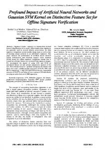
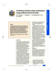
Fig. 1. Relation between inlet flowrate and d50c .

Most of the models have been derived by using multivariate analysis on the data which basically is generated by varying one variable and keeping other variables constant. This is exemplified in Fig. 1, which shows the relationship between the flowrates and the 50 . The data tested in this paper has been obtained from a closed circuit slurry test-rig. The slurry, mixed in a 500 L reservoir, made from 212 mesh ground silica particles, is circulated through the cyclone. Representative overflow and underflow samples of the slurry are taken simultaneously. The samples are then dried and analyzed by conventional methods using sieves. Over 200 data points has been obtained describing 50 and 50 values. Variables affecting 50 have been manipulated in a controlled and sequential manner.

0018–9456/97$10.00  1997 IEEE

EREN et al.: ESTIMATION OF HYDROCYCLONE PARAMETER

Because of the difficulties, all the conventional models are restricted to few estimation variables, such as the flowrates and densities of slurries, the height of vortex finder, the fixed dimensions, e.g., spigot opening, the pressure differences etc. Also, the empirical models may not be applicable universally since experimental conditions can change from one operation to another, this may explain the existence of many different formulae obtained under experimental similar conditions. Even using the same test rig it is difficult to keep consistent operations over a period of time, variables such as the solid contents and the particle size distribution within the slurry tend to fluctuate from time to time. In order to give a wider applicability to the conventional models incorporation of additional estimation parameters, such as water and solid split ratios, densities etc., is necessary but difficult to do so and also time consuming. In a recently published paper, Eren et al. [5] showed that an artificial neural network (ANN) can also be applied to estimate the 50 . In their paper, Eren et al. predicted 50 , obtained from the test rig described above, by using the same conventional parameters as appeared in literature. The predicted data by ANN correlated with the experimental results well, by giving a correlation coefficient of 0.986 and an r-squared value of 97.17%. These can be compared with conventional models, such as Eren’s model [1] which gives a correlation coefficient of 0.963 with an r-squared value of 96.66%. When Plitt’s model [2] is applied to the same data, somewhat poorer results are obtained, a correlation coefficient of 0.895 and an r-squared value of 80.14%. Nevertheless, it is worth highlighting that Plitt’s model might have given better results if the data obtained on their test rig was used. Among many other reasons, one of the important reason for obtaining poor correlation of data by conventional models is that these models fail to take into account the other essential variables which are likely to affect the 50 . In this paper, it will be shown that in addition to conventional variables, e.g., inlet flowrates, inlet density, spigot opening, vortex height, and temperature of slurry, other unconventional variables can also be included in the prediction of 50 . It will also be shown that by the application of ANN the correlation of the data can be improved substantially. The results obtained by ANN do not only yield to better correlations but also are much quicker and flexible to apply compared to empirical models. The ANN used in this study is the back propagated neural network (BPNN) [6]–[8]. The BPNN is widely used as supervised ANN. Supervised learning requires a set of training data which consists of a number of desired outputs and corresponding input data. The BPNN has a number of layers; one input layer; one output layer; and a few hidden layers. The objective of training BPNN is to adjust the weights between the layers such that application of a set of inputs produce the desired set of outputs. Calculations are done to obtain the output sets by processing through the input layers to the output layer, and then propagated back through the network. Although, BPNN is known to have some limitations it has been demonstrated to work successfully in many applications.

909

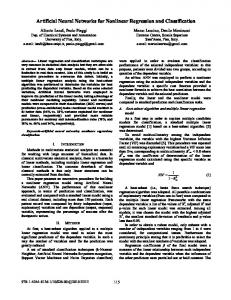
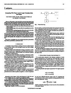
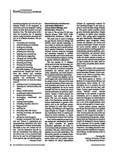
One advantage of BPNN is that it does not require much knowledge of the system before it can generate the desired output. BPNN can learn from the training examples such that the learning can be applied to new input data generated under similar operating conditions. Although, the training of BPNN is slow, once it has learned the outputs can be generate in a very short time. However, the selection of parameters for BPNN, such as the number of hidden neuron in the hidden layer, may require many tests to determine the best configuration. II. ADDITIONAL ESTIMATION PARAMETERS AND RESULTS When ANN is used, many other Hydrocyclone parameters effecting the 50 may be included as input variables. Fig. 2 illustrates the addition of three further parameters as the input variables. These parameters are the underflow and overflow flowrates and the ratios of the two flowrates. Further analysis indicated that the correlation coefficient of the trained results has increased to 0.995 giving an r-squared value of 98.9%. The 50 effectively represents the split of particles to underflow and overflow streams, therefore it is natural to expect that the ratio of the split of the liquid should play an important role in the efficiency. With the additional parameters, the ANN resulted in better correlation of the data, only in the expense of slight increase in the training time. However, the incorporation of the liquid split ratios to the conventional methods would have not been impossible but very difficult and costly. The prediction of the 50 can be enhanced by inclusion further relevant parameters. Fig. 3 depicts the trained ANN results with 14 input variables. In addition to the parameters used Fig. 2, others such as solid split ratios, the overflow and underflow densities and the pressure difference between the inlet and the overflow streams are included in obtaining Fig. 3. In this case, the correlation coefficient has further improved to 0.995 with an r-squared value of 98.97%. To fully utilize ANN once the network is trained the learning of the network is assumed to be holding for any future data generated under the same operational conditions. In order to verify this the network has been trained with some arbitrarily selected 50% of the data and the other 50% has been used for testing for the same input variables are as in those in Fig. 2. Typical results are illustrated in Fig. 4. In this example, the correlation coefficient is found to be somewhat reduced to 0.97 with an r-squared value of 96.67%. However, these results are still better compared to those predicted by classical formulae. In this figure it can be seen that there is a wide discrepancy in some of the results, which can be observed in run number 94 and 175, indicating that oscillations might have been taking place in the training. In obtaining this figure the following BPNN parameters were selected: hidden layer , hidden neurons , initial upper layer border , initial lower layer border , tolerance error 0.01, and maximum number of iterations . The training parameters were slightly modified to obtain the results in Fig. 5. The hidden neurons were increased to six, initial borders were reduced to 0.5 and the tolerance error was reduced to 0.0001. As it can be seen, the results

910


Fig. 2. The data and predicted results with eight parameters.

Fig. 3. The data and predicted results with 14 parameters.

improved considerably for a maximum iteration of 50 000. This indicates that the prediction accuracy of the BPNN is directly affected by the selection of parameters such as number of hidden neurons, the threshold training errors and the number of iterations as well as selection of appropriate input variables directly related to 50 .

In this application only one hidden layer has been selected in obtaining all the results presented above. As an outcome of this study, it is found that the training time increases as the number of input variables increase. In Fig. 2, training time was around 14 min with a mean square error per unit of 0.000 707. As expected, the time taken for Fig. 3 was the

EREN et al.: ESTIMATION OF HYDROCYCLONE PARAMETER

911

Fig. 4. The results with large prediction error.

Fig. 5. The results with improved training parameters.

longest at 20 min. However the mean square error per unit was 0.000 249. III. CONCLUSIONS In the prediction of Hydrocyclone parameter, 50 , the results of two best known conventional models have been

compared with those results obtained by application of ANN. It is shown that ANN yields to superior results which fits better with the original data. Unlike conventional models, ANN can easily incorporate additional operational variables of hydrocyclones to improve the fit. Performance of ANN can further be enhanced by careful selection of training parameters.

912


It is indicated that the use of ANN can lead to more effective and efficient automatic control of hydrocyclones. REFERENCES [1] A. Gupta and H. Eren, “Mathematical modeling and on-line control of hydrocyclones,” in Proc. Australia IMM, 1990, vol. 295, no. 2, pp. 31–41. [2] L. R. Plitt, “A mathematical model for hydrocyclone classifier,” CIM Bull., vol. 69, no. 776, pp. 114–122, 1976. [3] A. J. Lynch and T. C. Rao, “Modeling and scaling up of hydrocyclone classifiers,” in Proc. 11th Int. Mineral Processing Congr., Cagliari, Italy, 1975, pp. 245–270. [4] J. Mizrahi and E. Cohen, “Studies of some factors influencing the action of hydrocyclone,” Inst. Min. Met., pp. C318–330, 1966. [5] H. Eren, C. C. Fung, and A. Gupta, “Application of artificial neural network in estimation of hydrocyclone parameters,” in Proc. Australian IMM Annu. Conf., Perth, Australia, Apr. 1996, pp. 225–229. [6] D. E. Rumelhart and J. L. McClelland, Parallel Distributed Processing: Explorations in the Microstructure of Cognition. Cambridge MA: MIT Press, 1986. [7] P. Wasserman, Neurocomputing, Theory, and Practice. New York: Van Nostrand Reinhold, 1990. [8] S. T. Welstead, Neural Network and Fuzzy Logic Applications in C/C . New York: Wiley, 1994.

++

Halit Eren (M’87) received the B.Eng. degree in 1973, the M.Eng. degree in electrical engineering in 1975, and the Ph.D. degree in control engineering all from the University of Sheffield, Sheffield, U.K. Currently, he is the Head of the Department of Electronic and Communication Engineering, Curtin University of Technology, Perth, Western Australia. Previously, he lectured at the School of Mines, Kagoorlie, WA. His areas of expertise are control systems, instruments and instrumentation, mineral processing, signal processing, and engineering mathematics. His principle areas of research are ultrasonic and infrared techniques, density and flow measurements, moisture measurements, telemetry, telecontrollers, mobile robots, hydrocyclones, and artificial neural networks. He serves as a consultant to a number of industrial establishments.

Chun Che Fung (M’93) received the B.Sc.(Hon.) and M.Eng. degrees from the Institute of Science and Technology, University of Wales, in 1981 and 1982, respectively. He received the Ph.D. degree from the University of Western Australia in 1994. From 1982 to 1988, he was a Lecturer at the Singapore Polytechnic. In 1989, he joined the School of Electrical and Computer Engineering, Curtin University of Technology, Perth, Western Australia. His research interests are applications of computational intelligence to engineering problems. Dr. Fung is a member of the IEE and IEAust.

Kok Wai Wong (S’88–M’91) received the Diploma in electronics and communication engineering in 1991 from Singapore Polytechnic, and the Bachelor of Computer System Engineering in 1994 from Curtin University of Technology, Perth, Western Australia, where he is now pursuing the Masters degree. His research areas includes artificial neural networks, fuzzy logic, and their applications.

Ashok Gupta (M’97) received the B.Sc., M.Sc., and Ph.D. degrees from Sheffield University, Sheffield, U.K. He also attended the University of Minnesota, Minneapolis and the Ontario Research Foundation, Canada. He was Chemist in Charge at Burmah Oil Co. Ltd, India, then Assistant Technical Manager, and Manager Blast Furnaces, Indian Iron and Steel Co. Ltd., India. He was Senior Lecturer and then Principal Lecturer and Head of the Department of Metallurgy, School of Mines, Curtin University of Technology, Kalgoorlie, Australia. He is presently Director and Metallurgical Consultant with the Metals and Minerals Process Designing Consultancy, Perth, Western Australia. He has several publications in the fields of mineral processing, ferrous, and nonferrous extractive metallurgy. Dr. Gupta was a Colombo Plan Research Fellow.