Lagrange programming neural networks - IEEE Xplore

IEEE TRANSACTIONS ON CIRCUITS AND SYSTEMS-11: ANALOG AND DIGITAL SIGNAL PROCESSING, VOL. 39, NO. 7, J U L Y 1992

441

Lagrange Programming Neural Networks Shengwei Zhang and A. G. Constantinides Abstract-Most of the neural techniques for constrained optimization follow a penalty principle. However, it has been well known for a long time that penalty approach exhibits some vital deficiences. This paper analyzes in detail a class of neural networks appropriate for general nonlinear programming, i.e., problems including both equality and inequality constraints. The methodology is based on the Lagrange multiplier theory in optimization and seeks to provide solutions satisfying the necessary conditions of optimality. The equilibrium point of the network satisfies the Kuhn-Tucker condition for the problem. No explicit restriction is imposed on the form of the cost function apart from some general regularity and convexity conditions. The stability of the neural networks is analyzed in detail. The transient behavior of the network is simulated and the validity of the approach is verified with practical problem: Maximum entropy image restoration.

I. INTRODUCTION E research concerning analog computational circuits was dealt with as early as 1959 by Dennis [2l, and successive reports can also be found in the literature [13], [19]. The circuit was constructed by a dense interconnection of simple analog computational elements (neurons) and governed by a set of differential equations. Rather than solving an optimization problem by iteration using a digital computer, one can obtain the answer by setting up the associated neural circuit and measuring the node voltages after it settles down to an equilibrium point. Such circuits are particularly attractive in on-line applications with time-dependent cost functions. For many years, however, little attention has been paid to analog computational techniques, mainly due to the overwhelming advance of digital computers. Nevertheless, the bottle-neck phenomenon in digital computer forces people to turn to alternative techniques, and the success of artificial neural networks and the availability of VLSI techniques have intrigued interests of many researchers in applying neural computational prototype to practical optimization problems and further, in developing novel neural computational circuits. Neural circuit design techniques and related characteristic analysis is now becoming a typically challenging undertaking. In this paper we focus on the problem of systematically developing analog neural networks for nonlinear programming. Hopefield [lo] proposed an analog neural network which can seek for a minimum point of a quadratic energy

T”

Manuscript received February 20, 1991; revised December 19, 1991. This paper was recommended by Associate Editor Y.S. Abu-Mostafa. S. Zhang is with Expervision, San Jose, CA 95134. A. G. Constantinides is with the Department of Electrical Engineering,Imperial College, London SW7 2BT, UK. IEEE Log Number 9202009.

function. Since then various neural computational techniques have been reported [lo], [12], [141, [171, [20], [261, [27]. Most of the techniques, however, follow a direct decent approach and so is only suitable for optimization problems without any constraints. If the problem requires some equality and/or inequality constraints (general nonlinear programming), as would often occur in the real world, a penalty approach is usually employed, leading to a penalty function based on which a decent model is constructed. Such an approach, i.e., using a decent algorithm to solve a constrained problem via a penalty function, has been well studied in optimization theory and many helpful conclusions can be found in a text book picked up at random, (e.g. [l]).Under the condition that good initial information regarding the penalty parameter and starting point is available, the minimum point of the penalty function will reconcile the solution of the original problem. In the absence of good initial information, though, the penalty function approach should theoretically go through a sequence of unconstrained minimization of penalty functions with the penalty parameter increasing from the solution of each minimization phase, alternatively the suitable penalty parameter and starting point have to be found by trial-and-error. Both of the approaches are obviously not practical in real-time environments. Furthermore, there is always the evil of ill-conditioning bothering the penalty function approach. For a detailed discussion in this respect the reader is referred to [l, p. 1031. The above arguments justify the necessity to develop neural networks well suited for general nonlinear programming. L. 0. Chua and G. N. Lin proposed a canonical nonlinear programming circuit, which was aimed at solving nonlinear programming problems with inequality constraints [13]. The network was in simulating the Kuhn-Tucker condition from mathematical programming theory and can be realized with ideal diodes and nonlinear controlled sources. M. P. Kennedy and L. 0. Chua recast the circuit in a neural network paradigm and proved the stability of the circuit by presenting a co-content function as a Lyapunov function of the system [9]. The model is, however, primarily designed for optimization with inequality constraints. Direct application of the approach to equalities is likely to encounter technique problems since a circuit coupled with two inversed diodes can not work properly, though equalities can be mathematically expressed by a coupled sets of inequalities. In this paper we analyze a class of neural networks for nonlinear programming [3]-[51. The methodology is based on the well-known Lagrange multiplier method for con-

1057-7130/92$03.00 0 1992 IEEE

442

IEEE TRANSACTIONS O N CIRCUITS AND SYSTEMS-11: ANALOG AND DIGITAL SIGNAL PROCESSING, VOL. 39, NO. 7, JULY 1992

strained programming. Instead of following a direct descent approach of the penalty function, the network looks for, if possible, a point satisfying the first-order necessary conditions of optimality in the state space. There are two classes of neurons in the network, variable neurons and Lagrangian neurons, according to their contribution in searching for an optimal solution. Variable neurons seek for a minimum point of the cost function and provide the solution at an equilibrium point, while Lagrangian neurons lead the dynamic trajectory into the feasible region (the collection of all the points meeting the constraints). The Lagrangian neuron is treated on an equal basis with the variable neurons and the dynamic process is carried out simultaneously on both, in other words, both kinds of the neurons possess same temporal behavior. For most of the neural models, the cost function is most often embedded into the Lyapunov function of stability, which greatly restricts the applicable functional form. For example, in Hopfield's model, a quadratic cost function is usually required. The model discussed in the paper successfully separates the Lyapunov function from the cost function, thus freeing us from specific functional forms and enabling us to concentrate on general principles. The model described here adds to the known repertoire of neural circuits. The paper is organized as follows. In Section I1 we first illustrate the method by constructing a neural network for nonlinear programming with equality constraints, and discuss local and global stability of the network. A Lyapunov function is set up during the procedure. In Section I11 we discuss as special cases the rederivation of the backpropagation and the quadratic programming; much stronger conclusions are obtained for the latter. Experimental results including a simple example and the maximum entropy image restoration problem are presented in Section IV to illustrate the computational capacity of the network. Section V contains some concluding remarks. Appendix I completes the proof of the theorem in Section I1 and Appendix I1 extends the algorithm to general nonlinear programming with both equality and inequality constraints. 11. NEURALNETWORKS FOR NONLINEAR WITH EQUALITY CONSTRAINTS PROGRAMMING 2.1. Equality Constrained Problem Consider the following nonlinear programming problem with merely equality constraints:

(ENP)

Minimize f ( x )

tailed theoretic analysis. Denote the gradient of a scalar function s(x) as

where the superscript T indicates the matrix transposition. Definition I: Let x* be a vector such that h ( x * ) = 0. We say that x* is a regular point if the gradients Vh,(x* Vh,(x*) are linearly independent. The Lagrange multiplier approach is based on solving the system of equations which constitute the necessary conditions of optimality for the programming problem. Definition 2: The Lagrange function L : R " + m+ R is defined by ),.-a,

L ( x , A) = f ( x )

+ ATh(x)

(2-3)

where A E R" is referred to as the Lagrange multiplier. Denote

V,: L( x , A)

=

[

d 2 L ( x ,A) dXidXj

]

and

Vh

=

[Vh,;*.,Vh,].

We have following results from classical optimization theory [l,ch. 11. Proposition 1: Let x* be a local minimum for (ENP) and assume that x* is a regular point. Then there exists a unique vector A* E R" such that

V , L ( x * , A*)

=

0

(2.4)

and

z'V,',(x*, A*)z

2

0 , for any z withVh(x*)Tz = 0. (2.5)

Proposition 2: Let x* be such that h ( x * ) = 0. Assume that there exists a vector A* E R" such that V , L ( x * , A*)

(2.1)

=

0

(2.6)

and Subject to

h( x )

=

0

(2.2)

where x = ( x l , x 2 ; * * ,x , ) ~E R", f : R" + R and h : R" R" are given functions and m I n. The components of h are denoted hl;.., h,. f and h are assumed to be twice continuous differentiable. Before going further we introduce the regularity condition and some classical results, as a preparation for de--f

zTv,2,L(x*,y*)z > 0 for any z

#

0 with V h ( x * ) T z= 0. (2.7)

Then x* is a strict local minimum for (ENP). The first-order necessary condition of optimality can be expressed as a stationary point (x*, A*) of L ( x , A) over x

ZHANG AND CONSTANTINIDES:LAGRANGE PROGRAMMING NEURAL NETWORKS

and A. That is. V f ( x * ) + Vh(x*)A* = 0

V , L ( x * , A*)

=

V A L ( x * A*) ,

= h(x*) =

0.

(2.8) (2-9)

Or more precisely df(X*) dxi

+

AT-

dh(X*)

j=1

to their role in searching for the solution. In the dynamic process of the neural network, Lagrangian neurons lead the trajectory into the feasible region while variabk neurons decrease the Lagrangian function L ( x , A). The decrease of the Lagrangian function by x can be verified from the fact that along the trajectory of the network

1,2;.., n (2.10)

=

0, i

=

1,2;..,m.

=

443

dXj

h j ( x * ) = 0, j

(2.11)

The conventional approach is to solve the n + m equations defined by (2.10-2.11) with n + m unknowns, x l ; - * ,x , and AI,-.., A,,,, via a digital computer. Under the local convexity conditions of Proposition 2, the solution x* is a strict local minimum for (ENP). This approach will work well for a low dimensional problem, but not for a high dimensional one because of the limited capacity of memory and speed of a computer and the possibly illconditioning feature of the problem. For example, an image of size 512 X 512 has 218 pixels. Although many theoretically powerful procedures such as K-L transform, maximum entropy restoration, etc., can be posed as corresponding constrained optimization problems [23], they cannot be made concrete by simply solving tremendously high dimensional, and, in most cases, nonlinear systems (2.10-2.11). 2.2. Definition of the Network

Our aim now is to design a neural network that will settle down to an equilibrium point satisfying (2.8-2.9), or (2.10-2.11). The transient behavior of the neural network are defined by the following equations.

=

-

2 (2)’0. I

Remarks: 1) It is interesting to point out at this juncture the similarity between our nonlinear programming neural model and the activity transmission between the cortex and subcortical structure in human brains. There is evidence from neurobiology that the cortex has little intrinsic activity of its own, but the neurons of each small region independently fire in response to signals from elsewhere in the brain [8]. If such a role for the cortex is integrated into the general activity of the brain, one could argue that there is a continuous shuttling of activity between the cortex and subcortical structure [8, ch. 31. If we denote the current state of activity of the cortex as A and the subcortical structure as x , a simplified view of the cortex expressed above leads to a representation of the shuttling given below as a first approximation.

dx

- = F ( X , A)

dt

(2.12)

dA

- =h(x)

dt

dA

_ -- VAL( X , A) dt

e

(2.13)

If the network is physically stable, the equilibrium point ( x * , A*), described by ( d x / d t ) l , , t , A * ,= 0 a n d = 0, obviously meets (8) and (9) and thus (dA/dt)l(,*,A*, provides a Lagrange solution to (ENP). Expressing the definition (2.12) and (2.13) in component form, we obtain the Lagrange programming neural network (LPNN) described as follows. State equations:

=

1,2;.*, m

(2.15)

where x , , i = 1,2;..,n and Aj, j = 1,2,--.,rn are now assigned a physical meaning as neuron activities. The neurons in the network can be classified into two classes: variable neurons x and Lagrangian neurons A, with regard

(2.17) (2.18)

where F(x, A) and h ( x ) denote the information transfer function. This is surprisingly similar to our artificial neural network model. However, it is important to point out that there seem to be no sufficient reasons to argue that the functions F and g are gradients of some intrinsic function. 2) Geometric Explanation: A geometric explanation of the neural network is available due to the saddle point property of the optimal solution. We say that the saddle point property holds for L ( x , A) at ( x * , A*) if L ( x * , A) I L ( x * ,A*) I L ( x , A*).

dAj - - - h,, j dt

(2.16)

i= 1

(2.19)

The saddle point property is a sufficient condition for optimality ([7]). We claim that the neural network (2.14-2.15) tends to search for a saddle point of L ( x , A), provided that it starts from a nearby initial point. Indeed, if x is kept constant, the time derivative of L ( x , A) along the trajectory of the

IEEE TRANSACTIONS ON CIRCUITS AND SYSTEMS-11: ANALOG AND DIGITAL SIGNAL PROCESSING, VOL. 39, NO. 7, JULY 1992

444

network is

=

f2I:(

I=

2 0

(2.20)

of the network of an arbitrary value. One of the most effective approach for stability analysis is Lyapunov's method, in which the critical step is to find a suitable Lyapunov function. Fortunately, such a function exists for our network. Definition 3: The function E(x,A) is defined by

1

which when combined with (2.16) indicates that along the trajectory of the neural network the Lagrangian function is always decreasing with x and increasing with A, until the network reaches an equilibrium at which d L / d t l ( x * % A * ) = ( d L / d X ) ( d u / d t ) l ( x * , A*) + (dL/dA)(dA/dt)l,,., = 0. Thus (x*,A* ) is a saddle point of L(x,A).

2.3. Local and Global Stabilitv Suppose that x* is a local minimum point of f and A* is the associated Lagrange multiplier, we have shown that ( x * , A*) is an equilibrium point of system (2.14-2.15). While for the network to be of mactical sense, (x*,A*) should furthermore be asymptotically stable, so that the network will always converge to (x*, A* ) from an arbitrary initial point within the attraction domain of (x*,A*). With this in mind we state and prove the following theorem, which in other words represents the local stability of the network. Theorem I: Let ( x * , A*) be a stationary point of L ( x , A). Assume that V;,L(x*, A*) > 0 and x* is a regular point of (ENP). Then (x*,A*) is an asymptotically stable point of the neural network. Proof Following the procedure in nonlinear dynamic system theory [19] we consider linearizing (2.12) and (2.13) at the equilibrium point (x*,A*). The local characteristic of the equilibrium is determined by the linearized system. Taking V x L ( x * ,A*) = 0, h(x*) = 0 into account, the linearized system is given by

. (2.21)

0

Define V?*L(x*, A*) Vh(x*) G = [ -Vh( x * ) ~ 0

1

,

(2.22)

It is proved in the Appendix that the real part of each eigenvalue of G is strictly positive, which means that - G is strictly negative definite. And thus (x*,A*) is asymptotically stable (see for example [16, pp. 1131). When utilizing neural networks for optimization, we are usually much more interested in the global stability of the network. It is highly desirable that the network is globally stable in the sense that is will never disdav oscillation or chaos, starting from an arbitrary point. Thus an optimal solution can always be obtained by setting the initial state I

=

1 -IVf(x) 2

1

+ A T V h ( x ) I 2+ -Ih(x)(' 2

(2.23)

where 1 . I denotes the Euclidean norm. E ( ~A), is a L~~~~~~~function of the network under the convexity and regularity conditions stated in Theorem 2. Theorem 2: Suppose that the Hessian V:x L(x,A) is positive definite everywhere in the dynamic domain o f the network. Then the network is Lyapunov stable. Proof Differentiating E ( X , A) with respect to time t along the trajectory of the neural network gives

d E ( x , A)

-

dt

dE(x,A) du dx

-dt+

d E ( x , A) d A dA dt

drc =

[VxL(x,A)'V:,L(x,A) + h ( x ) ' V h ( x ) ] ~ dA + V'L(x, A)'Vh(x) Tdt

+ V x L ( x ,A ) ' V h ( ~ ) ~ h ( x ) =

- V x L ( x , A ) V ; x L ( ~A, ) 7 V x L ( ~A ),

(2.24)

where the last equality is correct since h(x>' V h ( x ) V x L ( x A) , is a scalar and h ( x l T Vh(x)V,L(x, A) = [h(x)' V h ( x ) V , L ( x , AllT = V , L ( x , A)' Vh(X)' h ( x ) . ( d E ( x , A))/dt is always negative when the Hessian V;',L(x, A) is positive definite in the dynamic domain. Obviously, E(x,A) 2 0 is lower bounded. Hence E ( x , A) is a Lyapunov function for the neural network and the neural network is Lyapunov stable. Corollary I : x tends to a limit x* at which V x L ( x * ,A) = 0. Prooj At the limit we have (dE(x,A)/dt = 0 which leads to V,L(x, A) = 0 due to (2.24) and the positivity of the Hessian. And so from the neural dynamic eauation (2.12) we have & / d t = - V x L ( x , A) = 0, hence x' tends to a limit x*. Corollary 2: Assume further that Vh,(x* Vh,(x*) is linearly independent. Then A also has a limit A*. Proof When V h ( x * ) is linearly independent, from V x L ( x * ,A) = Vf(x*) + V h ( x * ) A = 0 we can see that A is uniquely determined by the equation. Thus d A/dt + 0. Remarks: );.e,

0 in Theorem 1 can be weakened if the neural model is modified with the aid of the augmented Lagrangian function [11. Consider the following equivalent problem to (ENP): f(x)

minimize

1

+ -2- c ( h ( x ) l 2

subject to h ( x ) = 0

(2.25) (2.26)

where c is a scalar and I I again denotes Euclidean norm. Then an augmented Lagrangian function can be formed. L,(x, A)

=f

(x)

1

+ A T h ( x ) + -clh(x)l'. 2

except for some special cases (quadratic programming, for example). For most of real world problems, however, it is generally possible to justify from our prior knowledge that the problem is convex and the solution is unique. Thus we can employ the proposed neural network with confidence that it will finally reach the solution from arbitrary initial points. 111. APPLICATIONS

So far we have presented the model in an abstract manner. Now let us consider two applications of the model: rederivation of the back-propagation and the quadratic programming. 3.1. Redenuation of Back-Propagation

The back-propagation algorithm can be rederivated using the Lagrange multiplier. Assuming that x ( t ) represents the state of a vector of unit at instant t and D ( t ) is a desired target vector, the cost function can be written as

(2.27)

The modified neural network, which will be referred to afterwards as augmented Lagrange programming neural netowrk (ALP"), is specified by the following relation. State equations:

The network constraints are expressed as

x(t

=

1,2;.., n (2.28) (2.29)

A simple calculation shows that

V ~ , L C ( x *A*) ,

=

V 2 x L o ( x * A*) ,

+ c V h ( x * ) V h ( x * ) ' (2.30) = f ( x * ) + ATh(x*) = L ( x * , A*).

where L,(x*, A*) If c is taken sufficiently large, the local convexity condition can be shown to hold under fairly mild conditions [l]. This means that we can concexib our problem before employing the neural network. This technique is also theoretically valid for relaxing the condition for global stability, while the choice of c may not be so easy since the consideration would have to cover the whole dynamic domain. Even though the local convexity condition holds, the augmented Lagrangian function may still be quite useful in accelerating the convergence of the neural network. The relation between the convergence speed and the value of c will be discussed in detail in Section VI. Given a particular application, it might not be practical to verify that the sufficient condition of Theorem 2 is valid at every point in the dynamic domain

(34

where x(0) is the initial state, w is a weight matrix, and g is a differentiable function [28]. The Lagrangian L is L

i

+ 1) = g ( w x ( t ) )

=

E

+ C A T ( t ) [ x ( t )- g ( w x ( t ) ) ] .

(3.3)

It is easy to show that V L , = 0 gives a recursive rule to compute A(t) and that it is exactly the gradient of the back-propagation algorithm [28]. 3.2. Quadratic Programming In this case the network will be very simple; indeed it may even be a linear circuit (for problems with only equality constraints). The Hessian will be constant and thus it is easy to verify that the global stability condition holds. Moreover, quadratic programming is important in its own right; it arises in various applications where the cost, or error, is measured by the least square criterion. a ) Equality Constrained Quadratic Programming: Quadratic programming with equality constraints has the form of minimize f ( x) subject to

1

=

-xTQx 2

+ p'x

Ax = b

where x E R" is a variable vector, Q E R"'" is an symmetric, positive definite matrix, A E R"'" is of full row rank, and p E R", b E R" are constant vectors. The Lagrangian function now becomes L ( x , A) = (1/2)xTQx + p T x + A T ( h - b), where A E R"' is the Lagrange multiplier. Following the discussion in Section


446

11, the neural network is described by the equations,

is connected to p l , the output is y;, and it contains a self-feedback by (3.6b).

(3.4a) dh -=Ax-b. dt

(3.4b)

Or, in component form,

( 3S b ) where Q = (qi,), A = ( a i j ) , p i , and b, are the components of p and b, respectively. Since in this circumstance V:-L(x, A) = Q > 0 independent of x and A, the network is globally stable and the network exhibits a unique equilibrium point which provides the optimal solution to the problem. b) Inequality Constrained Quadratic Programming: The neural networks for quadratic programming with both equality and inequality constraints can be easily obtained following the discussion in Appendix 11, but we have no intention to explore in that direction further. Instead, let us consider neural networks for problems with only inequality constraints, so as to provide a comparison with those discussed above. The problem has the form 1 f( x ) = -xTQx + p'x 2 g(x) = A x - b I0.

minimize subject to

All the parameters are similarly defined for those with equality constraints. Following the discussion in Appendix 11, the neural network is described by the relation

U1

dYj _ dt

j=1

IV. COMPUTER SIMULATIONS In this section we will first present a simple example to illustrate the validity of the approach in solving optimization problems. While this is a simple example, it does serve to indicate the fundamental idea behind the approach taken, and help to obtain a deep insight into the transient behavior of the network described previously. The efficacy of the augmented Lagrangian function in accelerating convergence is also discussed. The capability of the network in dealing with realistic problems is then demonstrated with the applications of maximum entropy image restoration. 4.1. A Simple Example

The example is to minimize a quadratic function with equality constraints. Example 1: minimize

subject to

h,(x) =xI +x2 h,(x)=x,

+ 2x3 - 2 = 0

- ~ 2 = 0 .

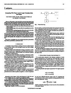
The neural network for this problem can be easily derived from (3.5). We have studied the transient behavior of the circuit from various initial states by simulating the dynamic equations via the classical fourth-order Runge-Kutta method [18] on a digital computer. The network converged to the global minimum point x* = (0, 0, which is the theoretical solution. Fig. l(a) shows a typical transient process of x1 corresponding to an initial condition x = ( - 1.0,2.0, - lS), A = (0.6, -0.3). 4.2. The Effect of the Penalty Parameter.

k=l

Let us now examine the effect of the penalty parameter -2pIyj,

j

=

l,...,m

(3.6b)

c in ALPNN. In Section 2.3 it was shown that the opti-

mization problem can be convexified by using an augmented Lagrangian function, leading to the ALP" b,, j = l ; . . , m . ( 3 . 6 ~ ) model. The condition for stability can be weakened in this way. In addition, ALPNN is of advantage in accelerating The network is also globally stable and has a unique the convergence. Fig. l(b) shows the transient behavior of equilibrium point following the fact that V,',L(x, A) = ALP" on example 1, with c = 1.0 and the same initial Q > 0, provided that the strict complementary condition condition as in Fig. l(a). Much improved behavior can be of Theorem 4 holds in the dynamic domain. observed. However, little difference is found when c is Comparing the network (3.6) with that defined by (3.3, further increased. This phenomenon can be understood we can see that these two kinds of networks display an from an analysis of the effect of the penalty parameter c. interchangeable structure. In hardware implementation The effect of c is to introduce a penalty ingredient into the network for inequality constrained problems can be the object function for any violation of the constraints. realized by simply "switching on" special neurons repre- When the initial state of the network is set at a random senting additional variables y, to the network for the point, it is very likely that the constraints are considerably corresponding equality constrained problems. These neu- broken. Thus a large value of c forces the state to rons are constructed as follows. The input of the neuron j approach the feasible region quickly. While after the state

I

447


x'[;p, ,

,

4 7 4

-1.20

0

4

0

12

I6

20

tlm.

an acceptable restored image. However, the validity of the simplifications are severely restricted in practice and the accomplishment of an algorithm is achieved only at the cost of quality decrease in restored images. A typical example is the well-known maximum entropy restoration procedure. Although it has been theoretically demonstrated to be extremely powerful in optical image enhancement and restoration, its applications are quite restricted simply because of its intensive computational complexity. However, in what follows we can see that the neural network provides a promising computational alternative. Image degradation in a linear system is generally characterized as [23]:

y

0.70

-0.06

-0.82

@ - - - - -- 1- . 2- +

1

tlm.

I

(b) Fig. 1. (a) The transient behavior of x 3 in Example 1. (b) The transient behavior of x 3 in ALPNN with c = 1.0 for Example 1.

is near enough to the feasible region, c has little effect on the behavior since the task of finding an optimal point now becomes much important. Very large c would also give rise to diversing. In our case it is empirically found that the diversing boundary is about c = 5. Experimental results also revealed that the ALPNN shows little improvement on convergence for those problems including some inequality constraints. This may be due to the high-order nonlinear characteristics of the corresponding neural networks, but the theoretical analysis is not available at this moment. 4.3. Using LPNN for Maximum Entropy Image Restoration

=

[ H ] X +V

(4.1)

where H is the point-spread function, X the original object distribution, V the noise, and y the recorded image. Given the recorded image y and the system feature [HI, the restoration problem is to find an acceptable solution X,with or without the knowledge on the noise process I/. Unfortunately, there would be no unique solution in view of noise and ill-conditioning; hence some meaningful rationale must be employed to pick a better solution. An important constraint is the maximum entropy criterion, and the restoration procedure can be described as [23]: M

Maximum

M

xi In ( xi) -

-

Subject to

y

-

[H]x -

uj

In (9) (4.2a)

j= 1

j= 1 U =

0

(4.2b)

M ..

CXj - I o =

0

(4.2~)

j= 1

where x = X + a , U = V + b, and a and b are small positive constants to shift X and V from their possible values of zero, so that ln(x,) and ln(uj) are well defined. 1, is a constant relevant to the sum of the gray level of the image y . Following (2.14) and (2.15), the LPNN for maximum entropy restoration is:

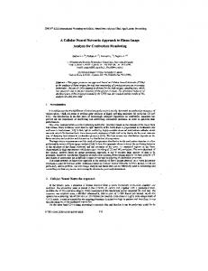
Image restoration is regarded as an important part of image processing. Generally speaking, the task of image restoration is to remove system degradation and noise so - = -(ln(x) -t 1) + [ H I T A - AM+, (4.3a) that the lost information is recovered as much as possible. dt All image restoration schemes can be virtually posed as du the solution of some particular optimization problem. (4.3b) - = -(ln(u) + 1) A Different choice of criteria or specific side conditions dt included as problem constraints will generate different dA restoration schemes. Many conventional methods, such as (4.3c) -= y - [Hlx- U dt Wiener filter, Kalman filter, maximum entropy, and leastsquares, can be found in the literature 1231. Though they (4.3d) are quite useful under some appropriate degradation models and noise assumptions, many of the methods suffer from the intrinsic high computational complexity where AT = ( A l , A*,..., A M ) , and ln(x) = ln(x,), and thus face limited applications. Some simplifications ln(x,);-., ln(x,). have to be presumed on the degradation model to make Fig. 2 presents the restoration result on grey level itself applicable to a particular algorithm and still obtain image of size 256 x 256, where (a> shows the degraded

+

~

448


(b)

Fig. 2. The restoration results on grey level images. (a) The image degraded by 1 X 7 uniform blur and -5.4-db SNR additive white Gaussian noise. (b) The restored image at 40 characteristic time of the network.

image, and (b) the restored image at the 40th iteration. The image in (a) is degraded by 1 X 7 uniform blur and -0.54-db SNR additive white Gaussian noise. The signal to noise ratio (SNR) is defined by (4.4) where q2 and U: are variances of signal and noise, respectively. The results in (b) are obtained by arbitrarily setting the initial states of all the variable neurons to 1/1024 and those of all the Lagrangian neurons to 0. The experiment demonstrates that, for equality constrained problems, the convergence is within 80 characteristic times of the systems, with the dimension of the systems varying from 5 as in Example 1 to 256 X 256 as in the image processing. In other words, the computation problem is solved in fewer than a hundred computational steps regardless of the dimensionality. VI. CONCLUDING REMARKS A novel kind of neural networks for constrained optimization has been analysed based on the well-known Lagrange multiplier theory. The equilibrium point of the circuit is shown to correspond to the Lagrange solution of the problem and is asymptotically stable under the regularity and convexity conditions. A Lyapunov function is established for the global stability analysis. The model is then successfully extended to general nonlinear programming with the aid of additional variables. There is no explicit restriction imposed on the functional form. The model exhibits remarkable capability in solving general nonlinear programming. Although it is primarily proposed for nonlinear programming, we believe that the model can be utilized for other applications such as associative memory; it even provides much more flexibility since the position of attraction points in the state space can now be adjusted by the Lagrangian neurons. Detailed analysis is still an open problem. The division of variable neurons and Lagrangian neurons is somewhat artificial, from a purely theoretical viewpoint. There is actually no difference in the temporal behavior of the neurons, and the dynamic process is

carried out simultaneously on both the variable and Lagrangian neurons. This feature provides speed potential over those models such as the dynamic-static circuit [26], in which the dynamics of constraint subnets have to be slower than that of the variable subnet to guarantee the dynamic stability. The penalty parameter c in the ALPNN is for convexifying the problem and speeding up the convergence. It is not essential if the problem is itself convex. We did not discuss the hardware implementation of the circuit in the paper. The reason lies in that the advance of artificial neural architectures is rapid and many choices are now available, such as the op-amp neurons by Kennedy and Chua [91, the CCD neurons by Agranat et al. [20], the integrator neurons by Yanai and Jawada [21], and the switched-capacitor neurons by Rodriguez-Vazquez et al. [12], to name just a few. This wide variety of implementations warrant the user's special consideration in practical environments. It is interesting to compare the model with that in [9]. For the latter, the constraints of the problem are never violated because of the use of nonlinear resistors, while for our model, the constraints can be violated during the dynamic process, but they are finally satisfied at the stable equilibrium point. This phenomenon may be viewed as a result of the soft-limiting principle of our approach.

MPENDIX I We show that the real part of each eigenvalue of G defined as G=[

Vh(x*)

V;',L(x*, A*) -

0

Vh( X* )'

1

T

(al.1)

is strictly positive definite provided that V:'L(x*, A* ) is positive definite. This claim can be found in [ l , ch. 41 but for reference convenience we present the proof here. We denote by 9 the complex conjugate of a complex vector y and Re( p ) the real part of a complex number p. Let a be an eigenvalue of G, and let ( z , w ) f (0,O) be a corresponding eigenvector where z and w are complex vectors of dimension n and m ,respectively. We have

while at the same time using the definition of G Re{['?'

;I)

$T]G[

=

R C { ~ ~ V : ~ L ( A*)z ~*,

+f'Vh(~*)~w Since we have for any real n

X

-

GTVh(x*)z}. (a1.3)

m matrix M

Re{ ~ ' M ' W } = Re{ GTMz)

T

(a1.4)

449


Proposition 3: Let x* be a local minimum for (GNP) and x* is a regular point. Then there exist unique vectors A* E R", p* E R' such that

it follows from (a1.2) and (a1.3) that Re{iTV,?,L(x*, A*)z}

$1)

=

Re([iTOT]G[

=

Re(a)(lz12 + 1 ~ 1 ' ) .

(a1.5)

V , L ( x * , A*,p*)

#

(al.6)

0

it follows from ( a 1 3 and the positive definiteness assumption on V,?, L ( x * , A*) that either Re( a ) > 0 or else z = 0. But if z = 0, the equation G[

$1

=

ff[];

(a1.7) (al.8)

Since V h ( x * ) has rank m it follows that w = 0. This contradicts our earlier assumption that ( z , w ) # (0,O). Consequently we must have R e ( a ) > 0. Thus the real part of each eigenvalue of G is strictly positive and hence G is positive definite. APPENDIX I1 We extend the design principle above to general nonlinear programming, i.e., problems including both equality and inequality constraints. The problem is initially converted into an equivalent one that includes only equalities so that the discussion in the previous section can be conveniently applied. A universal form of the problem can be expressed as (GNP) Minimize f ( x) Subject to

h ( x ) = 0, g ( x )

I

0

(a2.1)

where f : R" + R , h : R" + R", and g : R" + R' are given functions with m I n. The components of h and g are denoted by hl,..., h , and gl;.., g,, respectively. We assume that f , h , and g are twice continuous differentiable and g(x) is finite in the domain. Initially, the definition of a regular point has to be generalized. For any x satisfying the constraint g ( x ) I 0, we denote ~ ( x =) { j I g , ( x )

=

0,j

=

l;.*,r}

(a2.4)

(a2.2)

r/*I g1 ( x * ) = 0

j

=

I;.*,r. (a2.5)

Corresponding to the terminology of optimization theory, we define the following. Definition 6: A Kuhn-Tucker point of the optimization problem is defined as a point (x*, A*, p * ) satisfying the conditions below.

af(x*)

yields V h ( x * ) w = 0.

0,

r/; 2 0,

Since for any positive definite matrix A we have Re{iTAz} > 0 z

=

+

EA.fh1(x*) dx,

dx, = 0, i h l ( x * ) = 0, j

gk(x*)I 0, k pz >_ 0, k &gk(x*)

=

0 k

dgk(x*)

+

mdK,

k=l

=

l,...,n

=

l,...,m

(a2.6a) (a2.6b)

=

1;*-, r

(a2.6~)

1,s.. 7r

(a2.6d)

l;..,r.

(a2.6e)

= =

Our aim now is to design a neural network that will always converge to a Kuhn-Tucker point of the problem We transfer the inequality constraints into equalities by introducing additional variables: y,, i = l;.., r, and consider the following nonlinear programming problem that involves exclusively equality constraints. Minimize f ( x) Subject to h , ( x ) g,(x)

=

=

h,(x)

=

(a2.7)

0

+ y,2 = -.. = g,(x) + y,'

=

0. (a2.8)

The term y,' may be replaced by any differentiable positive functions of y , with suitable dynamic range. But for simplicity y,' is adopted in what follows. It has been proved from nonlinear programming theory that x* is a local (global) minimum point of (GNP) if and only if (x*, yy;-*,y:), where y,* = ,/j = 1,2,..., r, is a local (global) minimum of the transformed problem [l, ch. 11. The Lagrangian function L ( x , y , A, p ) given below is based on this conversion. Definition 7:

i.e., A ( x ) is the subset of indexes corresponding to the rn inequality constraints active at x. U x , Y , A, P ) = f ( x ) + h,h,(x) Definition 4: Let x* be a vector such that h ( x * ) = 0, 1=1 r g(x*) 5 0. We say that x* is a regular point if the + F](g,(X) +Y;). (a2.9) gradients Vh,(x*);.., Vh,(x*) and Vg,(x*), j E A ( x * ) , I= 1 are linearly independent. Definition 5: The Lagrangian function L ( x , A, p ) is deBy now we have defined two Lagrangian functions fined by L(x, A, p ) by (a2.3) and L ( x , y , A, p ) by (a2.9). Notice that V,L(x, y , A, p ) = V,L(x, A, p ) and V,?,L(x, y , A, p ) = L ( x , A, p ) = f ( x ) + A T h ( x ) + p T g ( x ) (a2.3) V;,L(x, A, p), as x and y are independent variables. The where A E R " and p E R ' are referred as Lagrange following discussion is based on the Lagrangian function multipliers. The following result is similar to that for L ( x , y , A, p ) of the transformed problem. A neural network can be specified for the equivalent equality constrained problems [l, ch. 11.

c

c

450


problem following the principle of the previous section. Note that x and y are primal variables and A, p are Lagrange multipliers. The dynamic equations can, therefore, be briefly written as

dx -=

- V x L ( X , Y , A, P )

f(X,Y) =f(x>

(a2.14) (a2.15)

) , j = l;.., m

hi( x , y )

= hi( x

gk(X,Y)

=gk(X)

(a2.10a)

dt ddt Y = - V , L ( X , Y , A, -

Next we define

(a2.10b)

P)

(a2.10~) dP _ - V,L(X, Y , A, P I

(a2.10d)

dt

+yk2,

,r

=

(a2.16)

and consider an equivalent problem minimize f (x, y ) subject to hi( x , y )

=

j = 1 , - . . , m ,k

0, g k ( x , Y ) =

=

0,

1,*--,r

or, in component form, State Equations

h i_ dt

df

dxj

dh. A-L j=l 'dxi

i

dgk -

=

k=l

P k z '

where f ( x , y ) , h j ( x ,y ) , & ( x , y ) are twice continuous differentiable due to the fact that f, hi, and gk are twice continuous differentiable. From Proposition 1 we have,

1,2;--, n (a2.11a) (a2.1lb)

dAj

-= hj(x), j dt

=

1,2,-..,m

(a2.1 IC) ( a2.1 Id)

V h ( x * ) T w= 0 , V g j ( x * ) T w + 2y7vj = 0, j

=

l,..., r (a2.18)

The transient behavior of the neural network seems quite intricate at first sight. Thus two questions will natu- where rally arise: 1) Does the steady-state of the system provide the optimal solution, or more precisely, the Lagrange D = (a2.19) solution to the problem? 2) Under what conditions does the network converge locally or globally? Theorem 3 makes certain that the equilibrium point of the neural network is always a Kuhn-Tucker point of the problem, For every j with y: = 0, we may choose wj = 0, 9 # 0 and U , = 0, for k f j, in (a2.17) to obtain py 2 0. For the thus justifying the optimality of the solution. Theorem 3: Let ( x * , y * , A*, p * ) be the equilibrium of j's with yy # 0 we already showed that p? = 0. This the neural network and assume that x* is a regular point. completes the proof. Theorem 4 illustrates that the Lagrange solution of the Then ( x * , y*, A*, p * ) is a Kuhn-Tucker point of the problem (GNP). problem is an asymptotically stable point of the network. Proofi Comparing Definition 6 with the neural dyTheorem 4: Let ( x * , y * , A*, p * ) be a stationary point of namic equation (a2.11) what remains to be proved is that L ( x , y , A, p ) such that V;?,L(x*,y*,A*, p * ) > 0. Assume that x* is a regular point and that the strict complementar$ g j ( x * ) = 0 and p; 2 0, j = l , * - * , r . Consider the equations ity condition ( p ? > 0 if j E A ( x * ) } holds. Then ( x * , y * , A*, p * ) is an asymptotically stable point of the neural network. Pro08 We consider only those y . , with j E A ( x * ) . For those y j with j not in A(x*), g j ( x ) # 0, thus py = 0 = g k ( x * ) + y z 2 = 0. (a2.13) according to Proposition 3. From the neural network dynamic equations (a2.11) we can see that y j , pj have no If pi # 0 then from (a2.12) y; = 0 and so is gk(X*) effect on other circuit variables in a infinite small region from (a2.13) Thus p g , = 0. Suppose that g k ( x * ) # 0 around Cy?, p;); they are isolated from other neurons then y z = 0 and thus & = 0 from (a2.12). and construct a stable self-loop. Thus they can be omitted These discussions confirm that p i g j , = 0 holds for all without affecting our conclusion. The linearized system at the equilibrium point cases.

,/mk#

~

451


(x*, y * , A*, p * ) is obtained as

V:x L ( x* , y * , A*, p* )

V,h ( X* , y * )

v,h ( x* ,y * )

0

-

1

always increasing with the rate - p k . Thus after some finite time d p k / d t = g k ( x ) + y i 2 0 and pk will be increasing until pk 2 0. However, if p k + 0, d y k / d t + 0 hence ( y k ,p k ) already settle down to an equilibrium ( y : , 0 ) and they do not involved in the transient behavior of other neurons. Consequently after a finite period we only need to consider the remaining circuit with these pk > 0, j = 1,2;.-, J. For this remaining circuit we define a function E ( x , y , A, p ) following the terminology in the proof of Theorem 4.

( a2.20)

+ -21I h-( x , y ) 1 2 . G=[

V : ? L ( ~ * , Y * ~, * , p * ) v , h ( x * , y * ) -V,h(x*, y * y 0

1

.

(a2.24)

Notice that the Hessian now becomes (a2.21)

d m ,

Then ( x * , y* 1, where y* = ( y T , * * *y:, ), Y,? = is a regular point since the gradients below can be easily verified to be linearly independent.

Thus from the discussion in the Appendix the positivity of matrix G depends on the positivity of matrix V&L(x*,y*,A*,p*)

=I

v ~ , ~ L ( x * , Y * , A * , ~ * o) 0

0

0

o ... ..- 2 4 ,

where k, E A ( x * ) ,j = l,...,J. G is strictly positive definite from the strictly complementarity condition as well as the strict positivity of V,??L(x*,y * , A*, p*). Hence - G is strictly negative definite and the point ( x * , y * , A*, p* ) is asymptotically stable. Theorem 5: Suppose that the Hessian V:x L ( x , A, p ) be positive definite and that the strict complementarity condition holds in the dynamic domain. Then the network is globally Lyapunov stable. Proofi It may well happen at the start that pk < 0 for some k . While from (a2.11b) it is easy to verify that y i is

It is easy to verify that E ( x , y , A, p ) is a Lyapunov function of the network following the similar procedure as in the proof of Theorem 2. Corollaiy 3: The state of the variable neurons, ( x , y ) , tends to a limit ( x * , y* ). Corollary 4: Assume that, in addition to the conditions in Theorem 5 , V h l ( x * ) ; . . , V h , ( x * ) and V g j ( x * ) , j E A ( x * ) are linearly independent. Then the state of the constraint neurons, A, p, have limits A*, p*. All the proofs for Corollary 3 and 4 are straightforward following Theorem 5 and Corollaries 1 and 2 of last section. Remark: From the proof of Theorem 5 the convergence of the network can be improved by replacing the term y i with a k y i , with ak > 1, k = 1,2,..., r in the definition of (a2.8). REFERENCES [l] D. P. Bertsekas, Constrained Optimization and Lagmnge Multiplier Methods. New York: Academic, 1982. [2] J. B. Dennis, Mathematical Programming and Electrical Networks. New York: Wiley, 1959. [3] J. C. Platt and A. Barr, “Constrained differential optimization,” presented at 1987 Neural Information and Processing Systems Conf. [4] -, “Constraint methods for flexible models,” Computer Graphics, vol. 22, pp. 279-288, 1988. [5] J. C. Platt, “Constraint methods for neural networks and computer graphics,” Ph.D. dissertation, California Institute of Technology, 1989. [6] D. P. Atherton, Stability of Nonlinear Systems. New York: Research Studies Press, 1981. [7] S. Vajda, Linear & Nonlinear Programming. London: Longman, 1974. [8] W. Ponfield and H. Jasper, Epilepsy and the Functionalhatomy of the Human Bruin. London: J. and A. Churchill, 1954. [Y] M. P. Kennedy and L. 0. Chua, “Neural networks for nonlinear

452

[lo] [ll]

[12]

[13]

IEEE TRANSACTIONS ON CIRCUITS AND SYSTEMS-11: ANALOG AND DIGITAL SIGNAL PROCESSING, VOL. 39, NO. 7, JULY 1992 programming,” IEEE Trans. Circuits Syst., vol. 35, pp. 554-562, May 1988. J. J. Hopfield, “Neurons with graded response have collective computational properties like those of two-state neurons,” in Proc. Natl. Acad. Sci., vol. 81, pp. 3088-3092, 1984. D. W. Tank and J. J. Hopfield, “Simple ‘neural’ optimization networks: An A / D convertor, signal decision circuit, and a linear programming circuit,” IEEE Trans. Circuits Syst., vol. CAS-33, pp. 533-541, May 1986. A. Rodriguez-Vazquez, R. Dominguez-Castro, A. Rueda, J. L. Huertas, and E. Sanchez-Sinencio, “Nonlinear switched-capacitor ‘neural’ netowrks for optimization problems,” IEEE Trans. Circuits Syst., vol. 37, pp. 384-398, Mar. 1990. L. 0. Chua and G. N. Lin, “Nonlinear programming without computation,” IEEE Trans. Circuits Syst., vol. CAS-31, pp. 182-188, Feb. 1984. L. 0. Chua and L. Yang, “Cellular neural networks: Theory,” IEEE Trans. Circuits Syst., vol. 35, pp. 1257-1272, Oct. 1988. 0. Barkan, W. R. Smith, and G. Persky, “Design of coupling resistor networks for neural network hardware,” IEEE Trans. Circuits Syst., vol. 37, pp. 756-765, June 1990. P. A. Cook, Nonlinear Dynamic Systems. London: Prentice-Hall International, 1986. C. R. K. Marrian and M. C. Peckerar, “Electronic ‘neural’ net algorithm for maximum entropy solutions of ill-posed problems,” IEEE Trans. Circuits Syst., vol. 36, pp. 288-293, Feb. 1986. L. V. Atkinson, P. J. Harley, and J. D. Hudson, Numerical Methods with FORTRAN 77. Wokingham, England: Addison-Wesley, 1989. T. E. Stern, Theory of Nonlinear Networks and Systems. New York: Addison-Wesley, 1965. A. J. Agranat, C. F. Neugebauer, R. D. Nelson, and A. Yariv, “The CCD neural processor: A neural network integrated circuit with 65536 programmable analog synapses,” IEEE Trans. Circuits Syst., vol. 37, pp. 1073-1075, Aug. 1990. H. Yanai and Y. Sawada, “Integrator neurons for analog neural networks,” IEEE Trans. Circuits Syst., vol. 31, pp. 854-856, June 1990. J. A. Feldman, “Connectionest models and parallelism in high level vision,” in Human and Machine Vision II. New York: Academic, 1985, pp. 86-108. T. S . Huang, Picture Processing and Digital Filtering. Berlin: Springer-Verlag, 1979. Y. Zhou, R. Chellappa, and B. K. Jenkines, “Image restoration

[25] [261 [271 [281

using a neural network,” IEEE Trans. Acoust., Speech, Signal Processing, vol. ASSP-36, pp. 1141-1150, July 1988. J. K. Paik and A. K. Katsaggelos, “Image restoration using the hopfield network with nonzero autoconnection,” in Proc. ICASSP ’90, pp. 1909-1912, 1990. Y. Yao and Q. Yang, “Programming neural networks: A dynamicstatic model,” in Proc. IJCNN, pp. 1-345-348, 1989. B. Kosko, “Bidirectional associative memories,” IEEE Trans. Syst., Man, Cybern., vol. 18, pp. 49-60, Jan./Feb. 1988. Y. LeCun, “A theoretical framework for back-propagation,” in D. Touretzky, G. Hinton, and T. Sejnowski, Eds., Proc. 1988 Connectionest Models Summer School, pp. 21-28, CMU, 1988.

Shengwei Zhang received the BSc. and M.Sc. degrees in electrical engineering from Tsinghua University, Beijlng, People’s Republic of China, in 1984 and 1987, respectively. Between 1989 and 1990 he was an academic visitor with the Department of Electrical Engineering at Imperial College, London. From October 1990 to December 1991 he was a research fellow with the Department of Electrical Engineering at Brunel University, London. He IS currently a research engineer with Expervision Inc. in California. His has published a number of papers on neural networks, image processing, and pattern recognition. His current interests include neural networks, optical character recognition, nonlinear optimization, and real-time learning.

A. G. Constantinides is a professor of signal processing at Imperial College, and he is also Head of the Signal Processing Section in the Department of Electrical Engineering. His current interests are in image and speech processing In neural networks, optimization techniques, communication theory and practice, and adaptive signal processing. he has published widely in the above areas. The Signal Processing Laboratory includes many other research activities under his direction Dr. Constantinides is a Fellow of the Institution of Electrical Engineers, and an honorary member of several international professional organizations.