DEFINITIONS AND MEASUREMENTS ... exist, the universal definition of Effective Resolution of .... complies with the best of currently used definitions (5) in.
12th IMEKO TC4 International Symposium, September 25−27, 2002, Zagreb, Croatia
ASPECTS OF ADC EFFECTIVE RESOLUTION: DEFINITIONS AND MEASUREMENTS Jan Holub, Josef Vedral Abstract − The article describes some aspects of understanding, defining and measurements of effective resolution of Analogue-to-Digital Converters. The disadvantages and misleading results of commonly used definition are shown and possible solutions are discussed. Finally, one new solution is given and arguments for its correctness and usability are collected. Keywords: ADC, effective resolution, effective number of bits 1. INTRODUTION Analogue-to-Digital Converters are used almost in all contemporary measuring devices to interface the analogue world (represented by chain: measured quantity, sensor, analogue pre-processing) and digital core of the instrument. Several parameters are used to describe ADC. Some of them refer to ideal behaviour of ADC (nominal number of bits, conversion rate), some of them refer to impairments of the real converter (Differential and Integral Non-linearity, Signal-to-Noise Ratio, Effective Number of Bits, Effective Resolution etc.). Although widely accepted standards [1,2] exist, the universal definition of Effective Resolution of ADC does not exist. 2. CURRENT STATUS To work further with description of ADCs, let us define the following terms: N-bit ADC with input range FS [V] has a quantisation step equal to
FS q= N 2
(1)
term Effective Resolution is obvious. The result, when given in voltage units (for ADC that deals with input voltage), should mean the rms value of smallest differences in input signal that could be resolved by the ADC, assuming that all code words and input signal slopes etc. has been covered/involved during the experiment. Moreover, it should be possible to recalculate the result to bits. In this case, for ideal ADC the result has to be again N. The factor determining effective resolution is noise, either quantisation noise or intrinsically analogue. Unfortunately, those simple requirements are not met by currently used definitions. The basic one that is rather misleading says [3] (3)
FS ER = log 2 RMS NOISE
where ER means Effective Resolution (bits) and RMS NOISE is rms value of noise on input of ADC converter. This is obviously wrong since numerator contains kind of peak-to-peak parameter and denominator contains kind of rms value. In the full paper, there will be shown an easy example (experimental results) how to obtain ER higher that is nominal number of bits N (of course without further signal processing like averaging). There were two attempts to improve this situation published [4], [5]. The first possibility deals with numerator modification. It assumes that the ADC converter is used to convert full-scale harmonic and the factor 2-1.5 is introduced to convert peak-to-peak value to rms value of corresponding harmonic signal:
FS ER1 = log 2
FS 2 2 = log 2 RMS NOISE RMS NOISE. 8
In case of ideal ADC, the value of Effective Number of Bits (ENOB) is equal to N. Otherwise ENOB is usually defined as [1]:
ENOB = log 2
FS
σ . 12
(2)
where σ means rms conversion error that in case of real ADC includes not only quantization error but also differential and integral non-linearity (and depends generally also on input signal frequency or occupied frequency band, respectively). Similarly, the intuitive understanding of the
(4) The alternative approach modifies directly denominator in order to change rms-type value to peak-to-peak-type value. It assumes uniformly distributed noise that allows to recalculate rms value to peak-to-peak value by means of multiplying by 12-0.5:
ER 2 = log 2
FS RMS NOISE. 12
(5)
12th IMEKO TC4 International Symposium, September 25−27, 2002, Zagreb, Croatia The noticeable similarity with ENOB definition (2) is interesting. This relation is applicable to the wider number of cases since the only condition of its applicability is the uniformity of noise distribution. There are no limitations or expectations given for input signal in this case. However, it is easy to understand that in case of e.g. normally distributed noise (Gaussian noise) such definition is useless because no peak-to-peak value is applicable. 3.
MEASUREMENT METHODS
The effective resolution can be determined either by suitable time-domain or histogram method. Goal of such measurement is the noise parameterisation. Histogram method allows determining even the amplitude distribution of noise. The common procedures will be described in the full text. 4.
NEW APPROACH
To overcome difficulties described in Paragraph 2, new definition has been developed. It requires knowledge of amplitude distribution of the noise. The basic idea is the modification of denominator of (5) and replacement of the constant 120.5 by other specific value, derived from the histogram by statistical uncertainty motivated approach. We are searching for the smallest interval Noisepp on noise probability density function characteristics that covers the required amount of occurrences, e.g. 95% or 99%. The size of this interval is then the denominator:
ER3 = log 2
FS Noise pp
(6)
Noise p-p occurances
For known (especially symmetrical) distributions, the value of Noisepp can be calculated directly form rms value of the noise by multiplication with the coverage factor k:
Noise pp = k .( RMS NOISE )
(7)
E.g. for normally distributed noise, one can use k=4 for 95% level of confidence or k=6 for 99% level of confidence. For uniformly distributed noise, the k=120.5 for 100% level confidence. For special types of distributions, the coverage factor has to be found using measured histogram case by case. Examples of calculation both for common and special amplitude distributions of noise will be shown in the full paper. Very short example is given in Tab 1. Tab 1. Various definition of Effective Resolution- result example (12 bit ADC, 10V full scale, ideal quantisation noise 705 µV RMS, total RMS NOISE 2.19 mV) 12.16 ER [bit] 10.66 ER1 [bit] 10.36 ER2 [bit] 10.36 ER31[bit] 10.16 ER32[bit] 1 0.5 – coverage factor 12 (uniformly distributed noise expected, 100% confidence level) 2 - coverage factor 4 (normally distributed noise expected, 95% confidence level) 5. CONCLUSIONS The general approach to definition of effective resolution of ADC was presented. The new generalised definition complies with the best of currently used definitions (5) in applicable cases but this new definition allows to determine correctly the effective resolution in wider amount of cases (virtually there are special requirements nor for ADC input signal nor for its noise).
100
REFERENCES 50
0 n-3
n-2
n-1
n
n+1
n+2
n+3
histogram code words
Fig.1 Histogram evaluation For symmetrical distributions, this algorithm leads always to single solution. For asymmetrical distributions, it is necessary to add the following artificial condition to avoid ambiguous solutions: The highest number of occurrences within the missed histogram bins should be minimal possible among all possible solutions (see Fig. 1).
[1] IEEE Standard 1057-1994, "IEEE Standard for Digitizing Waveform Recorders" [2] IEEE Standard 1241-2000, "IEEE Standard for Terminology and Test Methods for Analog-to-Digital Converters" [3] Analog Devices: “Practical Design Techniques for Sensor Signal Conditions”, p. 8.25, Analog Devices, USA, 1999 [4] Hejn, K., Pacut, A. and Kramarski, L., "The Effective Resolution Measurements in scope of sine-fit test," IEEE Trans. Instrum. Measur., vol. 47, pp. 45-50, Feb. 1998. [5] Vedral, J., Holub, J.: “Stochastic Testing Signals in ADC Testing”, Messtechnische Charakterisierung der AD-/DAUmsetzung, PTB, Germany, November 2000 [6] Guide to the Expression of Uncertainty in Measurement, ISO, BIPM, 1993, Switzerland