Network Deployments. Deepali Arora, Eamon Millman and Stephen W. Neville. Department of Electrical and Computer Engineering. University of Victoria.
2012 26th IEEE International Conference on Advanced Information Networking and Applications
Assessing the Expected Performance of the OLSR Routing Protocol for Denser Urban Core Ad Hoc Network Deployments Deepali Arora, Eamon Millman and Stephen W. Neville Department of Electrical and Computer Engineering University of Victoria P.O. Box 3055 STN CSC, Victoria, B.C., CANADA, V8W 3P6 {darora, emillman,sneville}@ece.uvic.ca minimum per-communication distance (or range) that preserve network-wide connectivity. This, of course, also comes at the trade-off of an increase in overall network latencies, thereby, leading to non-trivial design trade-offs. Innately, MANETs in which multi-hop communications dominate can achieve better network-wide capacities than networks in which 1 to 2 hop communications dominate. A careful study of prior MANET literature, particularly the studied node densities, movement models, and per-node communication ranges, shows that these prior works have primarily focused on assessing 1 to 2 hop MANETs and not the multi-hop networks that will likely be required within urban environments. These lower density network place limited stress on their underlying routing protocols as link breakages occur relatively infrequently. Overall, it is unclear from the existing literature whether the current MANET routing protocols will suffice for urban core smart phone-based MANETs. The literature suggest that Optimized Link State Routing (OLSR), a proactive routing protocol, will be the most suitable to these larger, denser networks, with comparisons of OLSR to a wider variety of other protocols having been studied in [2–15]. None of these prior works though has sought to assess OLSR’s performance within multi-hop networks. The specific question explored in this work are as follows:
Abstract—The wide-scale adoption of smart phones has begun to provide a pragmatic real-world deployment environments for mobile ad hoc networks, (i.e., as peer-to-peer game platforms, for emergency services,, etc.). Such deployments are likely to occur with urban cores where device densities would easily exceed those that have traditionally been studied. Moreover, the quality of the resulting solutions will innately rest on the capabilities of the underlying routing protocols. Of current protocols, the OLSR proactive routing protocol makes the strongest arguments regarding its suitability to such larger, denser network environments. This work tests OLSR’s true suitability by analyzing its performance within a 360-node network existing within a standard 1 km × 1.5 km communications area, (i.e., innately for a network with approximately 3 × the node densities typically studied). It is shown that OLSR largely fails for such denser networks, with these failure arising due to OLSR’s underlying presumption that routing tables updates should occur relatively infrequently. This limitation within OLSR has not been previously reported and this work highlights the reasons why these issues were likely not observed within prior OLSR studies.
I. I NTRODUCTION The wide-scale adoption of smartphones has begun to provide real-world ecosystems into which mobile ad hoc wireless networks (MANETs) can be pragmatically deployed, (i.e., to implement non-cellular based network services, peer-topeer game platforms, , etc.). MANETs solutions have been proposed for providing: useful applications in urban disaster recovery operations, connectivity in developing economies where standard infrastructure may be cost prohibitive or less available to user communities, and personal area networks (PANs) [1]. In general, such deployments would likely occur in urban cores and, hence, see the use of MANETs at scales and node densities that significantly exceed than what has been studied in the literature to date, (i.e., densities above the typical < 100 nodes per square kilometer of most studies). In such higher-density MANETs per-node communication distances must be reduced to maintain network-wide capacity, though obviously not to the extent that the network itself becomes disconnected. Fundamentally, in a broadcast medium decreasing per-node communication distances allows more nodes to communicate concurrently, (i.e., it reduces packetcollision rates and node-to-node interference levels). Hence, maximizing network-wide capacity requires the use of the 1550-445X/12 $26.00 © 2012 IEEE DOI 10.1109/AINA.2012.93
1) Does the OLSR perform as expected for higher density but stationary networks? 2) If yes, then how does OLSR’s performance change as node mobility is increased? 3) Can OLSR’s observed performance in the above situations be improved by adjusting its tunable parameters off of their widely known defaults? 4) Are the observed deficiencies in OLSR’s performance an artifact of the simulation approach used or are they intrinsic to OLSR itself? The approach taken to address these questions is to perform a rigorous set of statistically representative OLSR simulations using the OMNeT++ based simulation framework of [16]. This framework enables the exact re-running of suites of experiments under different OLSR parameter tunings, thereby allowing a direct and fair assessment of the impacts these retuning have on OLSR’s observed performance. 406
This paper is organized as follows. For completeness, the utilized simulation framework is discussed in Section 2, and an overview of the OLSR routing protocol is provided in Section 3. The applied statistical testing methodology of this study is presented in Section 4 with the experimental setup used for the conducted rigorous analysis of OLSR being presented in Section 5. The results of the conducted simulations and their analysis are then provided in Section 6. Section 7 then concludes the work.
performance within the urban core environments of particular interest within this work. The node mobility model used within this work is the random walk model. This model is chosen as it has been shown to provide a near-uniform stationary distribution of nodes in the modeled area. By comparison, such a critically important proof is not available and known not to occur for the widely used random way point model [20]. The radio propagation model is assumed to be a free space path loss model with path loss parameter α = 2. The standard constant bit rate (CBR) traffic model is used, in which fixed size packets are generated for delivery to new destinations after constant time intervals.
II. S IMULATION F RAMEWORK The system model used in this work employs a mixture of off-the-shelf resources and custom tools. The simulation model defining network area, node density, mobility, input traffic parameters, communication protocols and channel characteristics is designed by incorporating and/or modifying the existing modules available in the OMNeT++ simulation engine [17]. The simulations were carried out using a CentOS Linux cluster. The analysis was carried out using MatlabTM . The management framework used the Message Passing Interface (MPI) for inter-process communication which was implemented in Python. The network model considers a fixed 1500 m × 1000 m area in which 360 nodes travel, under a prescribed mobility model, where each node has a transmission range of 98 meters. Although there is no standard network size defined for MANET simulations [18] the combination of network area and transmission range has been selected to produce 78 neighbors per node (calculated following [18]) which is the optimum number of nodes required to produce a full connected stationary network [19]. The 98 meter transmission range ensures that the expected number of hops taken from source to destination ranges from four to six. This ensures that a multi-hop network is being studied and not the 1 or 2 hops networks of earlier studies involving smaller networks[3]. More directly, average hop count has not been specifically considered in earlier MANET studies, but as per Section 1 it is relevant in certain pragmatic situations. In small network studies, the per-node communication distances are typically quite large, (i.e., a significant fraction of the overall size of the communications environment). This results in all nodes being within 1 to 2 hops of all other nodes. Hence, nodes must be moving very quickly if network-level routes are to change during the period when any end node to end-node communication is occurring, (i.e., if the routing protocol is to be required to re-establish an in-use route). If the nodes move slowly in comparison to their per-node communication ranges and their expected end-point to end-point communication durations then, at the network-level, the MANET will appear to be nearly stationary, irrespective of what the actual per-node velocities may be. This innate underlying issue has not been well addressed or highlighted within the MANET literature to date. Overall a network that has a higher average hop count on an end-point to end-point communications basis will, therefore, place significantly more stress on its underlying routing protocol. Hence, studying multi-hop MANET scenarios provides a better assessment of the protocol’s likely true
III. OLSR
ROUTING PROTOCOL
The OLSR protocol [21] operates as a table driven, proactive protocol, in which topology information is regularly exchanged between nodes within the network. OLSR makes use of “Hello” messages as a mechanism for nodes to find their one and two hop neighbors. “Hello” message sender can then nominate a multipoint relays (MPR) as the one hop node that offers the best routes to its two hop nodes. OLSR uses topology control (TC) messages and MPR forwarding to disseminate the collected neighbor information throughout the network. In OLSR, nodes selected as MPRs are responsible for: forwarding the control traffic required to diffusion routing table changes throughout the entire network and, declaring link-state information for their MPR selectors. The main distinction between OLSR and reactive protocols, (e.g., AODV, DSR, , etc.) is that OLSR actively works to maintain the required routing tables within its MPRs ahead of their actual use by any of the nodes within the network, (i.e., node movements are actively tracked via the responses to the regularly transmitted “Hello” messages, thereby, enabling these proactive routing table updates). A. OLSR protocol parameters The performance of OLSR depends on the setting used for its configurable parameters. The primary settable parameters that directly influence OLSR’s behavior, as per [22], are: • Hello interval (HI) determines the time between the “Hello” messages that are used to keep track of the changes in the network’s connectivity. The standard default value is HI = 2 seconds [21]. • Refresh interval (RI) defines the minimum predetermined, period within which each link and each neighbor node must be cited. The default value is RI = 2 seconds with OLSR requiring that RI ≥ HI [21]. • Topology control interval (TCI) is the time period required for completion of the advertising of sets of available links. The default value is T I = 5 seconds[21]. • Neighbor hold time (NHT) denotes the duration for which information provided in a “Hello” message about link states and neighboring nodes should be considered valid. By default N HT = 3 × HI[21]. • Top hold time (THT) defines the period during which TC message information is considered valid. The default value is T HT = 3 × T CI[21].
407
Other parameters that influence the performance of the OLSR protocol include the multipoint relays (MPR) coverage, TC redundancy and willingness. The MPR coverage specifies the number of MPR nodes required to cover any strict 2hop nodes. The amount of information regarding MPRs or neighbors link state included in the TC messages of the local nodes is specified by the TC redundancy. Willingness defines how willing a node is to forward traffic. To retain reasonable limit on the number of simulation required, this work only focused on the varying of the HI, RI and TCI parameters across different MANET configurations. All other OLSR parameters are set to their default values. Varying HI and TCI, of course, also results in that varying NHT and THT, as per the above denoted default functional relations. It should be noted that just varying these three studied OLSR parameters results in a composite set of simulations that require substantial time on a computer cluster to run. A full analysis of OLSRs performance across the composite space of all of its tunable parameters would require substantial runtime within a larger-scale high performance computing facility. Whereas the more limited assessment provided in this work, suffice in the sense of highlighting OLSR’s issues when it is used within multi-hop MANETs. Finally, to ensure that the reported results are statistically valid only the portions of the produced simulation that produced statistically ergodic data are considered and compared. Innately, this is required as it makes no sense statistically to average or otherwise compare data that is drawn from different and distinct underlying distributions. The process by which this required statistical testing is done has been previously reported in [16] and, as such, is report below merely to provide completeness.
via applying statistical goodness-of-fit tests. Commonly used goodness of fit tests include the Kolmogorov Smirnov (KS) test, the Pearson’s Chi2 test, and the Anderson Darling test [25]. Within this work the two sample KS-test is applied to asses both the stationarity and ergodicity of the data produced via the OMNeT++ OLSR simulations. The two sample KS-test is a non-parametric test for assessing whether two empirical CDFs with high-likelihood been drawn from the same underlying distribution. This test is useful in the context of assessing OLSR’s performance issues as the underlying analytical distributions of the network-level MANET features of interest, as required by tests such as Pearson’s Chi2 test, are simply not known1. It should be noted that the KS-test is also a less powerful statistical test than either the Pearson’s Chi2 or the Anderson Darling test[25]; therefore, if a sample fails the KS-testing process then it will generally also fail these other tests. Hence, using the KS-test in this case can be viewed as being conservative in the sense of seeking to preserve data for subsequent analysis, where the general issue once such formal statistical testing is applied to MANET simulations is ensuring enough data survives for analysis and not excluding data due to its lack of ergodicity or its failure to settle out to a steady-state distribution, (i.e., its lack of stationarity). It should be clearly noted that passing statistical test for stationarity and ergodicity does not mean that the data is stationary or ergodic. Passing the tests only means that no evidence to the contrary exists at the tested confidence level. As is well known it is impossible to ascertain through data analysis whether a given set of data records have indeed been drawn from stationary or ergodic random processes.
IV. S TATISTICAL ANALYSIS
The process by which the stationarity and ergodicity testing is performed is best explained by considering a particular generic feature of interest, denoted X, that the researcher has instrumented the simulator to measure. Denote the ordered sequence of data regarding X produced during the nth run of the given simulation experiment by Xn = {hxj , tj i |j = 1, . . . , Jn }, where tj+1 > tj for all j ∈ {1, . . . , Jn − 1}. Denote the ensemble of data produced by the N experiment runs as X = {Xn |n = 1, . . . , N }. For simplicity, the xj will be assumed to be scalar, though the subsequent discussions can be trivially extended to the vector case. For each n ∈ [1, N ] it is assumed that different random seeds are used, (i.e., the goal is not to exactly reproduce the same experiment, which is not interesting statistically, but instead to assess the statistical nature of the experiments). Standard network simulators perform event-based simulations. Hence, the sample time τn = tj+1 − tj associated with any recorded Xn sequence is itself a random variable drawn from, in general, an unknown distribution. Moreover, eventbased simulations can be viewed as performing a form of important sampling in that the density of hxj , tj i tuples will be higher in more active, (i.e., interesting) areas (or times) of the
B. Testing for Stationarity and Ergodicity
Amongst other factors, the credibility of MANET simulations depend on the statistical validity [23] of the results obtained. Performing multiple simulations using different random seeds does not provide a guarantee of statistically rigorous results. Explicit testing for statistical stationarity (over time) and statistical ergodicity (across multiple Monte Carlo simulation runs) is innately required. A framework to support such testing has been presented in [16] and is used within this work. For completeness an overview of the statistical analysis carried out via this framework is provided as follows. A. Statistical Testing Overview A random process is considered to be stationary if its statistical properties (i.e., mean, variance, etc.) are time invariant. A stationary random process whose statistical properties do not differ when computed over different ensembles, (i.e., different Monte Carlo runs) is said to be ergodic. For ergodic random processes, the time averaged statistical properties are equal to their corresponding ensemble averages [24]. Stationarity and ergodicity can be directly tested for by comparing the empirical cumulative distribution functions (CDFs) produced over time and across an ensemble of Monte Carlo simulation runs, with these comparisons being done
1 Current theory does not provide derivations for what these distributions should be and, in general, the Central Limit theorem does not apply. Hence, presuming that the data will be Gaussian distributed is innately untenable.
408
where Wp denotes the employed widow width at the pth resolution level and is given by � � Texp ] , (3) Wp = 2p ∗ max[τn ] for p = 0, . . . , log2 [ 5
simulation. The stochastic nature of the simulations, implies that exactly when these interesting areas occur is likely vary from experiment run to experiment run. This creates the basic problem that Xn records cannot be directly compared due to their different random sampling rates τn . If what is of interest is X’s behavior over sufficiently long time periods, (i.e., periods T such that T >> max[τn |n = 1, . . . , N ]) then the Xn records can be converted to records with a common fixed sampling of T , denoted as the signals Xn (kT ), as follows:
Xn (kT ) = G[{hxj , tj i ∈ Xn |tj ∈ [kT, (k + 1)T )}]
(i.e., Wn1 is Xn cut up into windows of width max[τn ]. Wn2 has max[p] windows twice as large , etc., up to the point where Wn subdivides Xn into no fewer than 5 windows). KS-test is then used to test the sequence of windows in Wnp from back-tofront in terms of whether the sample cumulative distribution p function (CDF) for each Wq−1 window has, within a 95% confidence interval, been drawn from the same underling probability distribution as the sample CDF from the preceding Wqp window. To improve the statistical rigour of the stationarity testing, p if a given Wq−1 window of data passes the KS-test then the p next Wq−2 window is tested against the CDF formed as the average CDF from all of the preceding windows that iteratively passed the KS-test. As is well known in statistical analysis[26], this has the effect of reducing the uncertainty with respect to the estimated CDF to which the next window of data is compared. Hence, iteratively applying this process leads to the stationarity testing becoming increasingly rigorous as one moves from right to left through the windows of data. This testing process is begun with p = 0 and proceeds iteratively, until a sufficiently large set of Xn ’s recorded data, (e.g., ≈ 75%) passes the above KS-testing period, at which point tstat is set to the left boundary of the window with n the lowest q value that passed the KS-test. No testing is performed for higher p values as it is assumed that, given the characteristics of the data, if a smaller window width passes stationarity then larger windows will also pass and, thereby, these will generate similar values for tstat values. Additionally, n the tests becomes less rigorous as the window widths increase, given that the uncertainty in the CDF estimates innately increase with increasing window widths (i.e., the accuracy of the tstat values decreases with increasing p). If for all n p no windows pass the KS-test over a sufficiently large set of the Xn samples then the Xn record is marked as being non-stationary over its entire period, where this is distinct from setting tstat = Texp which would be fundamentally n incorrect. The overall stationarity testing process is illustrated in Figure 1. 2) Testing for Ensemble Ergodicity: The ergodicity testing proceeds after the stationarity testing has been performed. The ergodicity testing focuses on the sub-set of Xn records for which an associated tstat ∈ [0, Texp ] has been determined for n a given set of windows Wnp . Hence, the KS-test can then be applied down the ensemble on each of the n estimated CDFs produced from the stationary periods identified for each Xn record. In general, these per Xn stationary CDFs should be produced by averaging the CDF’s produced from the data held within each window within the Xn record’s Wnp stationary window set. If the stationary data from two Xn records is shown, at a 95% confidence interval, to have been drawn from the same underlying distribution by the KS-test then the two Xn records are denoted as being ergodic with each other but only within their [tstat n , Texp ] periods.
(1)
where G[.] can be any researcher chosen function that maps the set {hxj , tj i ∈ Xn |tj ∈ [kT, (k + 1)T )} to a point in X’s domain. In general, a typical example for such a function would be just replacing the PNset of tuples with its statistical average, (i.e., G[.] = N1 i=1 xi ). Alternatively, G[.] could denote xj ’s maximum value within the given interval, etc. This approach though cannot be used in general as it assumes that the time periods of interest, are much larger than the random sampling times τn and it assumes that the xj samples are relatively dense in the kT constant sampling periods, (i.e., that the statistic produced by G[.] has a sufficiently low degree of uncertainty2). As a number of the data records of interest in MANET simulations do not meet this condition, the following discussions regarding stationarity and ergodicity testing will presume Xn = {hxj , tj i |j = 1, . . . , Jn }, and that τn is a random variable of unknown distribution that varies with Xn i.e., Equation 1 does not apply. 1) Testing for per-Record Stationarity: The tests for stationarity focus on single Xn records and fundamentally, with respect to network simulations, asks: “When do the startup transients end?” Prior network simulation-based research has provided evidence that network simulations, particularly MANET simulations, initially have transient behaviors that settle out as the experiment runs, culminating in the experiment entering (or reaching) steady-state statistical behaviors at some point, denoted as tstat ∈ [0, Texp ], where the [0, Texp ] n interval denotes the full n-simulation run-time of the experiment in seconds. This observation provides the basis for the following stationarity test, the goal of which is to determine tstat statistically n for each of the N experiment runs. Given the above it can be assumed that the tail of the Xn record has a high likelihood of being stationary, whereas the head likely is not. Hence, the record Xn is iteratively cut up into a set of windows of data �� � � Texp (2) Wnp = Wq |q = 1, . . . , Wp 2 Any statistic produced via analyzing sample data records also has statistics, (e.g., its own mean, variance , etc.); hence, statistics produced via small data sets have high degrees of uncertainty when compared to properly produced statistics from larger data sets, presuming of course that sufficient statistics exist for the given feature’s underlying distribution.
409
Experiment Ensemble
{
mathematical operation on two other stochastic features then it becomes important that this composite feature is only computed within the ergodic regions common to the underlying features (or stationary regions if the composite feature in computed on a per Xn record basis). If this is not done then biases may be introduced into the reported analysis , (e.g., via the inclusion of start-up transients behaviors or the combining distinct behavioral modes).
x1(t) x2(t)
xN(t) t
0 sec
Texp
(a) The ensemble of records produced by N experiment runs for measurement feature X.
V. P ERFORMANCE MEASURES AND SIMULATION SETUP The affect of different parameter configurations on the performance of the OLSR protocol is assessed by analyzing quite standard four performance measures, namely: packet delivery ratio (PDR), delay after route establishment, hops traveled and routing overhead. The descriptions for each of these network-level features is as follows: • Packet delivery ratio (PDR) (fraction) is the ratio of the number of delivered application-level packets to number of sent application-level packets across the composite of the entire MANET. • Average delay after route establishment (seconds) is the total time that a packet takes to reach its end-point destination starting from when the route to this endpoint has been established. Not considered are the delays encountered while this route is being established, though for some protocols route recovery time may also be included as part of the average delay. • Hops traveled(number) is the number of hops packets take to travel from end-point to end-point of a given communication session. • Normalized routing overhead (measured as a percentage) is the number of packets required to establish MANET routes divided by the total number of packets during the MANETs operation. These four measures provide useful information required to assess the performance of any routing protocol and, except for hops traveled, are common measures in most studies [3]. Other measures such as throughput, maximum number of hops traveled by any packet, and end-to-end delay did not provide any new insights in OLSRs behavior and, hence, are not included in this work’s analysis. Monte Carlo simulations were performed across the four parameter configurations that are shown in Table I. The values of HI and TCI were varied as denoted for Configurations 1 to 4. Configuration 3 denotes the standard default OLSR configuration. Configurations 2 and 4 were chosen to assess the effect of reducing by half and doubling the values of TC and HI, respectively, over the default of configuration 3. A limitation arose in OMNeT++ OLSR implementation in that only whole numbers are allowed for the TCI and HI values. The results of the Configuration 2 experiments lead to including Configuration 1 in order to investigate the effect of using low and equal values for both TCI and HI (T CI = HI = 1).
Direction of KS-testing
}W }W }W }W }W }W
5 4 p 3 2 1 0 0
q
5 4 3 2 1 0
time
(b) The stationarity tests Wqp window tiling. KS-test CDF
CDF
KS-test CDF
CDF
KS-test Xn(t)
CDF
CDF
CDF
CDF
tnstat
(c) The KS-test stationarity testing process as applied right-to-left along an Xn record for a given set of W p windows.
Fig. 1: Illustration of the ensemble of records produced via rerunning a given experiment N times, showing Xn ’s random sampling intervals and the window tilings used for stationarity testing.
The set of N ensemble Xn records in X are then tested in a pair by pair manner to determine all sets of stationary data which are pair-wise ergodic. It is fully possible that more than one ergodic set of records may exist, (i.e., there may exist distinct modes of steady-state statistical behaviors within a given type of experiment leading to more than one ergodic region within the ensemble X). Currently, the testing framework reports the largest ergodic region found in X as X’s ergodic data. It should be noted that the ergodic (or stationarity) testing must be performed on a feature by feature basis, as ergodicity (or stationarity) for one feature, in general, provides no information about the ergodicity (or stationarity) of another feature. Moreover, if a composite feature is produced by a
VI. S IMULATION RESULTS Results are presented from the total of 350 independent Monte Carlo simulations that exhibited stationarity in each
410
TABLE I Parameter Hello interval (HI) Refresh interval (RI) Topology control interval (TCI) neighbor hold time (NHT) Top hold time (THT)
No. 1 1 1 1 3 3
0.6
0.01
0.4 0.3
0.008 0.006 0.004
0.2
0.002 5 10 Node Velocity (m/s)
0 0
15
5 10 Node Velocity (m/s)
(a) 120
5
Routing overhead (%age)
OLSR 1 OLSR 2 OLSR 3 OLSR 4
6 Hops travelled
15
(b)
7
4 3 2 1 0
No. 4 4 4 10 12 30
OLSR 1 OLSR 2 OLSR 3 OLSR 4
0.012
0.5
0.1 0
When the nodes are stationary in the sense of their mobility (i.e., zero node velocity) then the default configuration 3 and configuration 4 yield higher PDR than configurations 1 and 2. Innately, non-mobile or nearly non-mobile nodes do not require frequent updating of topology information to maintain network connectivity and, therefore, the default parameter values work well. Configurations 1 and 2 yield lower PDR because frequent updating of network routes is not necessary due to the near-zero velocity of the nodes, thereby creating an increased control packet overhead, observed as the lowered PDR values. As the node velocities are increased, however, link breakages become increasingly frequent requiring on-going updating of network topology information. As a consequence, configurations 1 and 2 yield higher PDR than configurations 3 and 4 for these higher node velocities. For stationary (0 m/s velocity) nodes, configuration 3 and 4 yield higher number of hops traveled (Figure 2c) and subsequently higher delays (Figure 2b) than configurations 1 and 2 indicating a more functional network for configurations 3 and 4. Lower hops traveled and delay for configuration 1 and 2 result from the frequent updating of topology information which, as discussed, produces higher routing overhead (Figure 2d). However, as node velocity induced link breakages increase, (i.e., as node velocities are increased), the number of hops traveled and delay reduces substantially for the configurations 3 and 4. This is a critical observation as it shows that for these configurations, increasing node velocities lead directly to a shattering of the MANET into a collection of numerous small local MANETs, (i.e., network-wide connectivity is lost and only 1 to 2 hop connectivity is preserved). This explains the low hop counts and decreased delays of Figure 2c and Figure 2b, respectively. The key issue highlighted here is that observing delay without respect to hops traveled can be misleading, as obviously a low delay is good but not when it comes at the cost of a disconnected network. It should be noted that increase in hops traveled innately leads to increased delay but the reverse is not true as delay increases can also occur irrespective of hops traveled, as per when a packet is held at an intermediate node while it tries to gain access to the communications channel. Configurations 1 and 2 are also adversely affected by increasing node velocities but are significantly less sensitive than configurations 3 and 4. Configurations 1 and 2 yield higher hops traveled and delay for 10 and 15 m/s node velocities indicating that a degree of MANET-wide connectivity is still maintained. The nearly double PDRs for configurations 1 and 2 (Figure 2a) at higher node velocities, of course, comes at the cost of increased routing overhead (Figure 2d). Overall, configurations with lower values of HI and TCI, i.e., Configurations 1 and 2, yield higher PDR, delay and hops traveled than Configuration 3 (the default) and configuration 4, for the tested higher node velocities because reducing HI and TCI increases the ability of OLSR to react to link failures thus allowing for better protocol performance. For stationary nodes, however, the default configurations yields a more functional network. Hence, a previously unreported dependency exists between the appropriate setting of the HI and TCI intervals and the expectation that link breakages will occur. This produces
0.014 OLSR 1 OLSR 2 OLSR 3 OLSR 4
0.7
Delay
Packet Delivery Ratio
0.8
Configurations No. 2 No. 3 1 2 1 2 2 5 3 6 6 15
5 10 Node Velocity (m/s)
15
OLSR 1 OLSR 2 OLSR 3 OLSR 4
100 80 60 40 20 0 0
5 10 Node Velocity (m/s)
(c)
15
(d)
Fig. 2: Effect of OLSR configurations on PDR, delay, hops traveled and routing overhead. OLSR 1-4 refers to OLSR with configurations 1-4 shown in Table 1.
of the above network-level features of interest. For the performance measures considered in this paper, the effect of using different OLSR configurations is assessed first. Second, the observed results for the performance measures are compared for a large (360 node) and a small (50 node) network to aid in identifying the limitations of the OLSR protocol. Finally, the effect of varying the values of parameters HI and TCI is investigated by keeping all other parameters fixed. For each experiment node velocities are varied across the range of 0, 0.5, 5, 10 and 15 m/sec. As varying data rate provided no new insights these results are not included. Generally speaking, for the performance measures considered significantly more sensitivity was shown to variations in node velocities than to any of the explored variations in data rates.
A. Effect of OLSR parameter configurations Figure 2 shows the effect of varying node velocities on the mean values of PDR, delay, hops taken and routing overhead, when using the different OLSR configurations for the denser 360 node multi-hop network using a fixed data rate of ∼ 90 KB/s. Figure 2 a shows that PDR decreases with increase in node velocity for all four configurations as a direct result of the increasing node velocities leading to increased occurrences of link breakages which, of course, adversely affects PDRs.
411
0.014
−3
0.6
0.01 0.6 0.4
0.008 0.006 0.004
0.2
5 10 Node Velocity (m/s)
0 0
15
(a)
Routing Overhead (%age)
Hops Travelled
3 2
5 10 Node Velocity (m/s)
(c)
15
4 5 10 Node Velocity (m/sec)
4 3 2
15
1 0
(d)
5 10 Node Velocity (m/sec)
(c)
Fig. 3: Comparison of PDR, delay, hops traveled and routing overhead for the large and small network
15
120 HI = 1, TCI = 1 HI = 2, TCI = 1 HI = 2, TCI = 5 HI = 1, TCI = 2
5
5
5 10 Node Velocity (m/sec)
(b)
6
OLSR Large Scale Network (360 node) OLSR Small Scale Network (50 node)
5 10 Node Velocity (m/s)
2 0
15
(a)
15
0 0
8 6
0.2 0.1 0
10
HI = 1, TCI = 1 HI = 2, TCI = 1 HI = 2, TCI = 5 HI = 1, TCI = 2
10
0.3
20
OLSR Large Scale Network (360 node) OLSR Small Scale Network (50 node)
4
1 0
15
x 10
12
0.4
(b)
6 5
5 10 Node Velocity (m/s)
0.5
Hops Travelled
0 0
0.002
14
HI = 1, TCI = 1 HI = 2, TCI = 1 HI = 2, TCI = 5 HI = 1, TCI = 2 Delay
OLSR Large Scale Network (360 node) OLSR Small Scale Network (50 node)
Routing Overhead (%age)
0.012
Packet Delivery Ratio
0.8
OLSR Large Scale Network (360 node) OLSR Small Scale Network (50 node)
Delay
Packet Delivery Ratio
1
15
HI = 1, TCI = 1 HI = 2, TCI = 1 HI = 2, TCI = 5 HI = 1, TCI = 2
100 80 60 40 20 0 0
5 10 Node Velocity (m/s)
15
(d)
Fig. 4: Comparison of PDR, delay, hops traveled and routing overhead for the large network using different values of HI and TCI
the observed dependence between PDR and routing overhead and the node velocities, with node velocities in the 2-3 m/s range, (i.e., slightly above average human walking speed) leading to a collapse of denser OLSR MANET employing default configurations. This collapsed network issue can be resolved by decreasing the HI and TCI setting but only at the cost of substantially increasing OLSR overheads. That OLSR effectively becomes non-functional in denser networks as node velocities increase has not been previously reported and is a critical issue if OLSR were to be used to support MANETs within urban core settings.
to converge for both networks. This is a further indication that, under configuration 3, the larger network becomes broken into many small networks and, as such, not surprisingly now reports measures more consistent with those of the 50 node network. The obvious conclusion being that communication across the full 360 node network is no longer possible, (i.e., the network has shattered due to OLSR in configuration 3 being unable to keep up with the pace at which route between nodes are changing). Finally, the routing overhead of the small network is much smaller than for the large network as would be expected (Figure 3d). A higher fraction of packets is required in the large network for route establishment because of the presence of multiple routes. It should be noted that this also would lead to higher reliability for the larger network, an issue not directly assessed in this work. For both the large and small networks routing overhead appears to asymptotically converge to an almost constant value as node velocity increases, as seen earlier in Figure 2d.
B. Effect of network size Figure 3 compares the effects that varying node velocity has on PDR, delay, hops traveled and routing overhead for both the tested 360 and a more standard 50 node networks under default Configuration 3 that has traditionally been used in a large number of network simulation studies. A fixed data rate of ∼ 90KB/s was used. Figure 3a shows that PDR decreases as node velocity increases for both the large and small networks due to the increased occurrences of link breakages, as seen earlier in Figure 2a. Also, the default Configuration 3 yields much lower PDR for the large network than for the smaller network. Innately, in the large network, to retain networkwide capacity, packets have to on average travel more hops to reach their destination than in the small network. Thus they are more likely to be lost due to effects such as link breakages. This causes the observed decreases in the PDR. For higher node velocities PDR drops substantially for the large network indicating a non-functional network, as discussed earlier for configuration 3. The delay and the average number of hops traveled by packets in the small network (Figure 3b and Figure 3c) are low when compared to those of the large network. As the node velocity increases both the delay and hops traveled tend
C. Effect of TCI and HI Figure 4 assesses the effect of using different values of HI and TCI on the four performance measures for the 360 node network and data rate of ∼ 90KB/s. Four different configurations of HI and TCI are used to gain insight into their relative effects on network performance. The first configuration uses HI = 1, TCI = 1. The second configuration uses HI = 1, TCI = 2 and thus allows to assess the effect of increasing TCI. The third configuration uses HI = 2, TCI = 1 and assesses the effect of increasing HI compared to the first configuration. The last configuration is the default configuration with HI=2, TCI =5. In all simulations, the refresh interval (RI) is set equal to HI and THT and NHT are varied according to the OLSR protocol specifications. 412
Two primary inferences can be drawn from Figure 4. First, for non-mobile nodes the default configuration (HI = 2, TCI = 5) yields higher PDR, delay, hops traveled and low routing overhead than other configurations with lower values of HI and TCI. In contrast, at higher node velocities the default configuration generally yields the lowest observed PDR, delay, hops traveled values. These results are similar to ones presented in Section 6A indicating that at higher node velocities frequent updating of network routes (i.e. higher routing overhead) is required if the network is to maintain network-wide connectivity. Whereas, when node velocities are low, at the network-level routes rarely, if ever, change thereby allowing high values of HI and TCI to be used. Additionally, this leads to configurations with lower values of HI and TCI having, overall, less sensitivity to changes in node velocities. Second, in regard to OLSR’s sensitivity to changes in its HI and TCI parameters, Figure 4 suggest that certain performance measures such as PDR and hops traveled are fairly sensitive to both TCI and HI values while other performance measures such as delay and routing overhead show more sensitivity to either HI or TCI, respectively. These observations directly contrast published studies that suggest that OLSR network behaviour is relatively insensitive to changes in TCI [27], [22]. This distinction primarily arises due to the prior works’ implicitly having studied OLSR’s behavior within the context of MANETs that placed limited stress on the routing protocol and where link breakages would have occurred relatively infrequently. As discussed, such scenarios are not the likely scenarios within MANETs structured to function within urban cores. Obviously, real-world MANET deployments can also, in most cases, be augmented through fixed access point (AP) infrastructures, with disaster recovery being the potentially atypical case. From this perspective, the issues highlighted within this work can be seen as helping to denote the node densities that would be supportable under any given AP and the assumed node mobility profile and node-level network traffic usage patterns, i.e., the assessments conducted can be viewed as being associated to a given AP service region. Moreover, alternatively how the OSLR network shatters with increased node mobility can be used to provide information regarding the optimal placement of APs for a given mobility model and node level network usage patterns. Space limitations preclude a fuller more detailed discussion of these issues within this work.
Results show that for low- to zero-velocity nodes the default parameter configuration (HI = 2, TCI = 5) yields higher PDR, delay, hops traveled and lower routing overhead than configurations with lower values of these parameters, as these low node velocities result in a network that does not require frequent route updates. As node velocity are increased, the default values of HI and TCI lead to a non-functional OLSR network that has been shattered into numerous small networks. This results from OLSR’s inability, at its default HI and TCI parameter setting, to keep pace with the rate at which the velocity induced link breakages and network topology changes are occurring. For higher node velocities, lower HI and TCI values can be used to yield network that better retains its network-wide connectivity. But, this improvement comes at the expense of increased routing overheads. In general, the reported results suggest that OLSR is most appropriate for networks in which node velocities can be (or are known to be) constrained to below 2 to 3 meters per second. This velocity limit can be increased by increasing the per-node communication ranges, but at the cost of significantly decreasing the network-wide capacity, (i.e., the number of nodes that can communicated concurrently within the network). Results of comparing the large and small networks under OLSR’s default parameter configuration, especially in terms of hops traveled and delay, suggest that for higher node velocities, the larger network essentially collapses into several small independent networks where communication is only maintained between neighboring nodes. Comparison of the results using different values of HI and TCI suggest that OLSR networks are sensitive to changes in both TCI and HI with different performance measures showing different sensitivities to these parameters. This contradicts earlier studies which suggest that OLSR-based networks are relatively insensitive to TCI changes. This difference arises as these prior studies did not test OLSR within the context of multi-hop network and, instead, primarily focused on network in which 1 to 2 hop communications dominated. Comparison of OLSR’s performance with its default parameter configuration for the tested large and small networks clearly shows that assessments conducted with respect to only a small networks are likely to yield a more optimistic assessments. As shown by the hops traveled results, the observed failure of the OLSR routing protocol is most likely due to the inherent nature of larger-scale denser MANETs and not simply an artifact of the simulation process as conducted or the simulator used. Hence, in part, due to the applied statistical testing approach the observed issues would not be addressable via simple fixes to the simulator or conducted simulation process. That these issues have not been previously reported for OLSR is merely a result of the nature of the networks used in the prior studies. The innately conclusion of this work is that OLSR is likely not an appropriate protocol to use for urban core MANETs as protocol causes failures in the MANET that would begin to appear as sufficient numbers of users begin to move at speed just over average human walking speeds.
VII. C ONCLUSIONS OLSR is considered to be one of the most suitable routing protocol for larger and denser ad hoc networks and significant work has been done to assess its performance. However, most earlier studies only considered small-scale networks that do not allow for a more comprehensive assessment of OLSR’s performance. This work has shown that OLSR’s performance within larger, denser networks and, particularly, networks structured to required multi-hop communications differs substantially from what has been reported in these earlier studies.
413
R EFERENCES [1] P. J. M. Frodigh and P.Larson, “Wireless adhoc networking-the art of networking without a network,” Ericsson review, 2000. [2] M. Rahman and A. Al Muktadir, “The impact of data send rate, node velocity and transmission range on QoS parameters of OLSR and DYMO MANET routing protocols.” 10th international Conference on Computer and Information Technology. ICCIT 2007., pp. 1–6, Dec. 2007. [3] A. Al-Maashri and M. Ould-Khaoua, “Performance analysis of manet routing protocols in the presence of selfsimilar traffic,” Proceedings of 31st IEEE Conference on Local Computer Networks, pp. 801 –807, Nov. 2006. [4] P. Sholander, A. Yankopolus, P. Coccoli, and S. Tabrizi, “Experimental comparison of hybrid and proactive manet routing protocols,” MILCOM 2002. Proceedings, vol. 1, pp. 513–518, July 2002. [5] F. Yongsheng, W. Xinyu, and L. Shanping, “Performance comparison and analysis of routing strategies in mobile ad hoc networks,” International Conference on Computer Science and Software Engineering, vol. 3, pp. 505–510, Dec. 2008. [6] H. Ashtiani, M. Nikpour, and H. Moradipour, “A comprehensive evaluation of routing protocols for ordinary and large-scale wireless manets,” IEEE International Conference on Networking, Architecture, and Storage, pp. 167–170, Nov. 2009. [7] C. Mbarushimana and A. Shahrabi, “Comparative study of reactive and proactive routing protocols performance in mobile ad hoc networks,” in 21st International Conference on Advanced Information Networking and Applications Workshops, AINAW ’07., vol. 2, 2007, pp. 679–684. [8] N. Shah, D. Qian, and K. Iqbal, “Performance evaluation of multiple routing protocols using multiple mobility models for mobile ad hoc networks,” in IEEE International Multitopic Conference, INMIC, 23-24 2008, pp. 243 –248. [9] A. Klein, “Performance comparison and evaluation of aodv, olsr, and sbr in mobile ad-hoc networks,” in 3rd International Symposium on Wireless Pervasive Computing, 7-9 2008, pp. 571–575. [10] J. Hsu, S. Bhatia, K. Tang, R. Bagrodia, and M. Acriche, “Performance of mobile ad hoc networking routing protocols in large scale scenarios,” in IEEE Military Communications Conference,MILCOM 2004., vol. 1, 31 2004, pp. 21 – 27 Vol. 1. [11] S. Hosseini and H. Farrokhi, “The impacts of network size on the performance of routing protocols in mobile ad-hoc networks,” in Circuits,Communications and System (PACCS), 2010 Second Pacific-Asia Conference on, vol. 1, aug. 2010, pp. 18 –22. [12] F. Maan and N. Mazhar, “Manet routing protocols vs mobility models: A performance evaluation,” in Ubiquitous and Future Networks (ICUFN), 2011 Third International Conference on, june 2011, pp. 179 –184. [13] J. Nakasuwan and P. Rakluea, “Performance comparison
[14]
[15]
[16]
[17] [18]
[19]
[20]
[21]
[22]
[23]
[24] [25]
[26]
[27]
414
of aodv and olsr for manet,” in Control Automation and Systems (ICCAS), 2010 International Conference on, oct. 2010, pp. 1974 –1977. G.K.Walia and C.Singh, “Simulation based performance evaluation and comparison of proactive and reactive routing protocols in mobile adhoc networks,” International journal of Computer Science and Information Technology, vol. 2, no. 3, pp. 1235–1239, 2011. P. Kuppusamy, K. Thirunavukkarasu, and B. Kalaavathi, “A study and comparison of olsr, aodv and tora routing protocols in ad hoc networks,” in Electronics Computer Technology (ICECT), 2011 3rd International Conference on, vol. 5, april 2011, pp. 143 –147. E. Millman, D. Arora, and S. Neville, “STARS: A framework for statistically rigorous simulation-based network research,” in IEEE Workshops of International Conference on Advanced Information Networking and Applications (WAINA), March 2011, pp. 733 –739. Omnet++. [Online]. Available: www.omnetpp.org/ S. Kurkowski, T. Camp, and M. Colagrosso, “MANET simulation studies: the incredibles,” SIGMOBILE Mob. Comput. Commun. Rev., vol. 9, no. 4, pp. 50–61, 2005. E. Royer, P. Melliar-Smith, and L. Moser, “An analysis of the optimum node density for ad hoc mobile networks,” IEEE International Conference on Communications, ICC 2001., vol. 3, pp. 857–861, 2001. M. McGuire, “Stationary distributions of random walk mobility models for wireless ad hoc networks,” Proceedings of the 6th ACM international symposium on Mobile ad hoc networking and computing, MobiHoc ’05, pp. 90– 98, 2005. P. J. T. Clausen, “Optimized link state routing protocol (OLSR),” Internet Draft, www.ietf.org/rfc/rfc3626.txt, Oct. 2003. C. Gomez, D. Garcia, and J. Paradells, “Improving performance of a real ad-hoc network by tuning olsr parameters,” in Proceedings of 10th IEEE Symposium on Computers and Communications, 2005, pp. 16 – 21. T. Andel and A. Yasinsac, “On the credibility of manet simulations,” Computer Communications, vol. 39, no. 7, pp. 48–54, July 2006. P. Z. J. Peebles, Probability, Random Variables, And Random Signal Principles. McGraw Hill, 2001. B. Lemeshko, S. Lemeshko, and S. Postovalov, “Comparative analysis of the power of goodness-of-fit tests for near competing hypotheses. 1. the verification of simple hypotheses,” Journal of Applied and Industrial Mathematics, vol. 3, no. 4, pp. 462–475, 2009. J. S. Bendat and A. G. Piersol, Random Data: Analysis and Measurement Procedures. Wiley-Interscience; 3rd edition, 2000. Y. Huang, S. Bhatti, and D. Parker, “Tuning olsr,” in Personal, Indoor and Mobile Radio Communications, 2006 IEEE 17th International Symposium on, 11-14 2006, pp. 1 –5.