Chris J. Garrett, Sergio B. Guarro, and George E. Apostolakis. Abstract- The Dynamic Flowgraph Methodology (DFM) is an integrated methodological approach ...
IEEE TRANSACTIONS ON SYSTEMS. MAN. AND CYBERNETICS. VOL. 25. NO 5, MAY 1995
824
The Dynamic Flowgraph Methodology for Assessing the Dependability of Embedded Software Systems Chris J. Garrett, Sergio B. Guarro, and George E. Apostolakis
Abstract- The Dynamic Flowgraph Methodology (DFM) is an integrated methodological approach to modeling and analyzing the behavior of software-driven embedded systems for the purpose of reliability/safety assessment and verification. The methodology has two fundamental goals: 1) to identify how certain postulated events may occur in a system; and 2) to identify an appropriate testing strategy based on an analysis of system functional behavior. To achieve these goals, the methodology employs a modeling framework in which system models are developed in terms of causal relationships between physical variables and temporal characteristics of the execution of software modules. These models are then analyzed to determine how a certain state (desirable or undesirable) can be reached. This is done by developing timed fault trees which take the form of logical combinations of static trees relating system parameters at different points in time. The prime implicants (multi-state analogue of minimal cut sets) of the fault trees can be used to identify and eliminate system faults resulting from unanticipated combinations of software logic errors, hardware failures and adverse environmental conditions, and to direct testing activity to more efficiently eliminate implementation errors by focusing on the neighborhood of potential failure modes arising from these combinations of system conditions.
I. INTRODUCTION
E
MBEDDED systems are systems in which the functions of mechanical and physical devices are controlled and managed by dedicated digital processors and computers. These latter devices, in turn, execute software routines (often of considerable complexity) to implement specific control functions and strategies. Embedded systems have gained a pervasive presence in all types of applications, from the defense and aerospace to the medical, manufacturing, and energy fields. The great advantage of using embedded systems is in the almost unlimited flexibility provided by the software implementation of system control functions and by the computational power and speed of modern microprocessor devices. As a result, very sophisticated and complex logic can be executed by relatively inexpensive microprocessors loaded with the appropriate software instructions. The originally implemented logic can also be modified at any point in the life of the system it is designed to control by uploading new software instructions. Due to this power and flexibility, embedded systems are increasingly being used in a number of safety critical applications. They have long been a feature of flight control systems and weapon control systems in the Manuscript received November I , 1993; revised July 3, 1994. Thc authors are with the School of Engineering and Applied Science, University of California, Los Angeles, CA 90024- 1.597. IEEE Log Number 9409224.
aerospace and defense industries, and they are now finding safety critical uses in many other fields as well [ 11-[7]. While the cost-effectiveness and flexibility of embedded systems are almost universally recognized and accepted, it is also increasingly recognized that the task of providing high assurance of the dependability and safety of embedded system software is becoming quite difficult to accomplish, due precisely to its very complex and flexible nature. Software, unlike hardware, is unique in that its only failure modes are the result of design flaws as opposed to any kind of physical mechanisms such as aging 121. As a result, traditional safety assessment techniques, which have tended to focus upon physical component failures rather than system design faults, have been unable to close the widening gap between the extraordinarily powerful capabilities of modern software systems and the levels of reliability which we are capable of exacting from them. Currently, embedded system software assurance is not treated much differently from that of any other type of software for real-time applications (such as communications software). Three principal types of software assurance philosophies can be recognized in the published literature, which are briefly described and discussed below. Assurance by testing, with or without the aid of reliability growth models is the most common approach. Testing is often performed by feeding random inputs into the software and observing the produced output to discover incorrect behavior. Because of the extremely complex nature of today’s modern computer systems, however, these techniques often result in the generation of an enormous number of test cases [ 3 ] . Software reliability models have been proposed to aid the development of testing strategies [81-[ IO], although the applicability to software of reliability models extrapolated from the hardware reliability realm is seriously questioned, even from within the software reliability research community itself [ 1 I ] . Formul verijccition is another approach to software assurance which applies logic and mathematical theorems to prove that certain abstract representations of software, in the form of logic statements and assertions, are consistent with the specifications expressing the desired software behavior. Recent work has been directed at developing varieties of this type of technique specifically for the handling of timing and concurrency problems [ 121, [ 131. However, the abstract nature of the formalisms adopted in formal verification make this approach rather difficult to use properly by practitioners with non-specialized mathematical backgrounds. The third type of approach to software assurance is one that analyzes the timing and logic characteristics of software
00 18-9472/95$04.00 0 IO95 IEEE
GARRETT C I til.: DYNAMIC FLOWGRAPH METHODOLOGY
executions by means of discrete state simulation models, such as queue networks and Petri-nets [ 141-[ 171. Simulated executions are analyzed to discover undesirable execution paths. Difficulties arise from the “march-forward’ nature (in time and causality) of this type of analysis, which forces the analyst to assume knowledge of the initial conditions from which a system simulation can be started. In large systems, many combinations of initial states may exist and the solution space may become unmanageable. A different approach, which reverses the search logic by using fault trees to trace backward from undesirable outcomes to possible cause conditions, offers an interesting solution to this problem, but encounters difficulties due to limitations in its ability to represent dynamic effects. and to the fact that a separate model needs to be constructed for each software state whose initiating causes are to be identified [IS], [ 191. An important open issue in embedded system assurance analysis is the issue of modeling and representation of hardwarekoftware interaction [20]-[221. The approaches to software qualification that have been proposed and/or developed in the past generally follow the philosophy of separating out the hardware and software portions of the assurance analysis. The hardware reliability and safety analysts evaluate the hardware portion of the problem under the artificial assumption of perfect software behavior. The software analysts, on the other hand, usually attempt to verify or test the correctness of the logic implemented and executed by the software against a given set of design specifications, but do not have any means to verify the adequacy of these specifications against unusual circumstances developing on the hardware side of the overall system, including hardware fault scenarios and conditions not explicitly envisioned by the software designer. Another important issue that needs to be addressed in the modeling and analysis of embedded systems is the dynamic nature of their behavior. For the purpose of simulating such behavior, and especially the discrete event transitions that occur in their software, discrete state transition models, such as queue networks and Petri-nets, have been proposed and applied with a good degree of success [ 151-I 181. The Dynamic Flowgraph Methodology (DFM) addresses these issues within a modeling and analysis environment in which system models are built which express the logic of the system in terms of causal relationships between physical and software variables [23]-[29], while the execution of software modules is represented as a series of discrete state transitions. The models are then analyzed to determine how the system can reach a certain state by backtracking through the model to develop fault trees. Fault tree analysis is very well established in the areas of safety and reliability analysis. Originally developed at the Bell Laboratory, fault tree analysis has been used to analyze nuclear power plants [30] and chemical processes [31], as well as software [18]. DFM represents a major step forward with respect to conventional fault tree analysis for three reasons. One reason is that DFM produces a self- contained system model from which many fault trees can be derived via algorithmic procedures suited for semi-automated computer implementation. A second reason is that the DFM representation is based on multi-
825
valued parameter discretization and logic, and, accordingly, the analytical insight of the fault trees derived from a DFM analysis is not limited by the constraints of the binary logic representation of conventional fault tree analysis. Methods for finding the prime implicants of multi-state logic fault trees have been identified and discussed in the literature [32],[33]. The third, and perhaps foremost reason why DFM represents a major evolution in system failure analysis capabilities over conventional fault tree analysis, is that it can produce “timed fault trees, that is, fault trees in which timing relations between key system and parameter states are systematically and formally taken into account. A timed fault tree takes the form of a combination of time-stamped pieces of conventional “static” fault trees which describe system parameter states at different time steps. In other words, a timed fault tree can be viewed like a series of snapshots of the system evolution, with each snapshot presented as a piece of a conventional fault tree, and with all significant time transitions explicitly identified within the logic structure of the tree, so that the existence of certain logic relations among system states across time boundaries, and the existence of certain timing conditions which are necessary to produce the fault tree top event, are also explicitly and unequivocally identified. This constitutes a significant advancement beyond conventional static fault trees in the representation of time dependence. In conventional fault trees, only the probabilities of occurrence of events may exhibit time dependence. In timed fault trees, on the other hand, the events themselves are also time dependent. Section I1 of this paper provides a detailed description of DFM, illustrating how system models are built, and how timed fault trees are developed by backtracking through those models. Section 111 illustrates the application of DFM to the problem of validating the design of a simple embedded system. Finally, Section IV discusses how the results of a DFM analysis are utilized, by identifying and removing catastrophic system failure modes and by developing efficient testing strategies which are targeted directly toward ensuring that such failures do not occur. 11. DESCRIPTION OF DFM
A . Overview This section describes, in detail, the Dynamic Flowgraph Methodology (DFM). The discussion begins with an overview of the methodology’s basic features, and then proceeds to describe the six fundamental elements of the DFM modeling framework (the process variable node, the causality network, the conditioning network, the transfer box, the transition box and the decision table), and illustrate how they are used in the analysis of an embedded system. The application of DFM is a two-step process, as follows: Step 1: Build a model of the embedded system for which a dependability analysis is required. Step 2: Analyze the model to produce fault (or success) trees which relate the events, in both the physical system and the software, which can combine to cause system failures, including the time sequences in which they occur, and identify
X?h
IEEE TRANSACTIONS ON SYSTEMS. MAN. AND CYHtRNbTICS. VOL. 25. NO. 5. MAY 1995
system failure (success) modes in the software and associated hardware as prime implicants of the timed fault (success) trees. The first step consists of building a model that expresses the logical and dynamic behavior of the system in terms of its physical and software variables. The second step uses the model developed in the first step to build timed fault (or success) trees that identify logical combinations of hardware and software conditions that cause certain specific system states of interest, and the time sequences in which these conditions come about. These system states can be desirable or undesirable, depending on the objective of the analysis. This is accomplished by backtracking through the DFM model of the embedded system in a systematic, specified manner. The information contained in the fault trees concerning the hardware and software conditions that can lead to system states of interest can be used to uncover undesirable or unanticipated software/hardware interactions, thereby allowing improvement of the system design by eliminating unsafe software execution paths. and to guide functional testing to focus on a particular domain of inputs and system conditions. DFM models take the form of directed graphs. with relations of causality and conditional switching actions represented by arcs that connect network nodes and special operators. The nodes represent important process variables and parameters, while the operators represent the different types of possible causal or sequential interactions among them. DFM’s usefulness as a tool for the analysis of embedded systems derives from its direct and intuitive applicability to the modeling of causality driven processes. DFM models provide, with certain limitations, a complete representation of the way a system of interconnected and interacting components and parameters is supposed to work and how this working order can be compromised by failures and/or abnormal conditions and interactions. The application of DFM to a simple hardware system is illustrated in Fig. 1. where a valve is used to control a downstream flowrate. In Fig. l(a), a piping and instrumentation diagram (P&ID) is drawn to describe the functional layout of the system, its components, and other elements of basic engineering data regarding the process. Other important attributes, most notably the ones linked to operational logic and control modes as well as the analyst’s own understanding of the system, while not directly contained nor implicitly expressed in the P&ID, are nevertheless represented in the DFM model of the system (Fig. I@)). The DFM model is built F. F M . ar.d 1.X as continuous with physical parameters variable nodes, where L’P: Upstream pressure, F : Flow rate, F M : Flow rate measured, t - X : Current Valve position, and S F and C F as discrete variable nodes, where: S F : Sensor state, C F : Control Function. The relationships between parameters are represented by gains in transfer boxes, which may be different for different conditions. Edges connect nodes through transfer boxes. An example of how relationships are represented in the DFM
model is the direct proportionality relationship between nodes
l i p and F. This is represented by a “/” in the transfer box between the nodes. The two nodes are connected through the transfer box using directed edges (Fig. I(b)). According to the different degraded states of the flowrate sensor, SF. (the sensor may fail high, fail low, etc.) the relationship between the nodes E’ and F M may change. This is clearly shown in the model (Fig. I(b)). It should be noted that the results of a DFM analysis are obtained in the form of fault trees, which show how the investigated system/process states may occur. DFM thus shares, in the final form of the results it provides, many of the features of fault tree analysis. The difference, however, is that it provides a documented model of the system’s behavior and interactions, which fault tree analysis does not provide nor document directly. The most important feature of this methodology is that it is possible to produce, from a single DFM system model, a comprehensive set of fault trees that may be of interest for a given system. This is a most useful feature since, once a DFM model has been developed, it is not necessary to perform separate model constructions for each system state of interest (as is the case in fault tree analysis). Because DFM modeling focuses on parameters, rather than components, it also offers greater modeling flexibility than fault tree analysis, although this flexibility goes along with proportionately more complex modeling rules and syntax. In Fig. I(c), the fault tree for the top event, “flow rate is high,” is derived. By working backward through the DFM model starting from the flow rate node F. we can determine that the state, “flow rate F is high,” is caused by either “upstream pressure U P is high” A N D “the valve opening is nominal,” OR “the valve is completely open.” This information is implicitly contained in the DFM input operator before the node E’. Underlying this input operator is a decision table constructed by determining the states of F from the combinations of the states of U P and V S . Thus, given a particular state of F. the information organized in the decision table can be used in reverse to determine the combinations of IIP and I-X which cause this particular state of F. This information is explicitly denoted in the resulting fault tree by connecting events with logical A N D and OR gates. Backtracking then continues until basic events are reached. To the extent to which it would be applied for systems which do not depend significantly on software, DFM is functionally equivalent to the Logic Flowgraph Methodology (LFM), a tool for computer-automated failure and diagnostic analysis. Details and examples concerning the application of LFM can be found in 1231-1291. An important issue that needs to be addressed in the mode!ing and analysis of embedded systems is the dynamic nature of their behavior. For the purpose of modeling such behavior and representing its effects in the system fault trees, the execution of software is modeled as a series of discrete state transitions within the DFM model. The usefulness of this approach is that i t provides the ability to represent changes in the system logic at discrete points in time. This allows the development of fault trees which reflect static relationships between the variables at different points in time.
GARRETT ef rrl
’
DYNAMIC FLOWGRAPH MkTHODOLOGY
827
7 UP
&
F
‘
B 0 Sensor
I a. Process ANALYSIS FOREVENTA
U
1 F]
b. DFM MODEL I
ANALYSIS FOR EVENT B
I
I Fig. I .
F1 F
= 10
: etc.
c . FAULTTREES
Example of DFM model and fault analysis
E . Step I: Model Construction I ) CausaliQ and Conditioning Networks: To implement the first step of DFM, a model that expresses the logical and dynamic behavior of the embedded system is constructed. The model integrates a “causality network” which describes the functional relationships among hardware and software parameters, a “conditioning network” which represents discrete software behaviors due to conditional switching actions and discontinuous hardware performance due to component failures, and a “time-transition network” that indicates the sequence in which different software subroutines are executed and different control actions are carried out. Embedded system software is generally real-time control software which receives real-time data from the physical part of the system and performs appropriate control actions on the basis of this data. The first step in modeling this type of software is to identify those portions of it which explicitly involve time dependencies, such as interrupts and synchronization routines. In most cases, the majority of time dependencies are present in the controlling, or “main,” module, however other modules may contain time-dependent elements and one must make sure that they are isolated. The remainder of the code, which has no real time dependence other than its own execution time, is divided into modules which represent physically meaningful actions. An examination of
the specifications, data dictionary, structure chart or even the code itself, if it has been written, will usually suggest an appropriate division of modules. The control flow among the above defined software “components” is then represented by a state transition network, in which the execution of each particular software component is represented by a transition between states. Associated with each transition is a time which represents the execution time of the software routine to which it corresponds. The modeling of the data flow between the software components is completely analogous to the modeling of causality flow. Associated with each transition in the state transition network is a DFM transfer box which, instead of describing a one-to-one causal relationship between physical variables, describes, in general, several many-to-one mappings between the corresponding software component’s inputs and outputs and any relevant global variables. It is here that the judicious division of the software into components becomes important. Each software component should correspond to a physically meaningful action, so that intermediate variables which do not correspond to any physical quantity are not involved in the transfer box mapping. By eliminating the need for the inclusion of intermediate variables from the software model, the mapping between the input and output variables produces an effective and relatively simple representation of
828
I M E TRANSACTIONS ON SYSTEMS, MAN, A N D CYBERNETICS. VOL. 25, NO. 5. MAY 1995
the software component. This approach permits relatively easy backtracking through the model for the purpose of building fault trees. The state transition network is then incorporated into the DFM model of the hardware system by modeling the causeand-effect relationships between the software variables and physical parameters. The principal step in the integration of the software and hardware portions of the model is the identification of all data that is exchanged between the software and the physical world, i.e., the identification of all of the software “images” of hardware parameters and physical variables. Corresponding parameters are then connected through a transfer box and an edge which indicates the direction of information How. In almost all cases, an interface point is constituted either by a sensor that measures a physical parameter to be input to the software or an actuator which translates a software command into a physical movement. Thus, one has to include in the hardware portion of the model nodes representing both the measured physical parameter and the associated measurement, or the software command and the actuator movement, respectively. The sensors and actuators themselves will be modeled as transfer functions normally representing direct proportionality but also containing conditional faulted mappings which represent different degraded states. The software portion of the model will begin with the measured value nodes which represent the images of physical parameters which are used as input to the software and end with the software commands which are output to the actuators. It is also important to note that, in addition to having a direct causal effect on the physical system via sensor measurements and actuator commands, software actions will, in general, also have an indirect effect on the physical system by conditionally changing the gains between physical variable nodes. This will occur whenever software controls the functions of physical devices such as pumps, valves, etc.. and is modeled by edges connecting the relevant software variable nodes with the transfer boxes in question. The building blocks of the “causality,” “conditional,” and “time-transition” networks in a DFM model are process variable nodes, transfer boxes, transition boxes, and decision tables. The building blocks are described below, and the manner in which these building blocks are assembled to form the three networks are discussed. 2 ) Process Variable Nodes: Process variable nodes represent physical and software variables that are required to capture the essential causal and conditioning behaviors of the system. A variable represented by a node is discretized into a number of states. The reason for the discretization is to simplify the description of the relations between different variables. This will become clear in the discussion of decision tables. The number of states for each variable must be chosen on the basis of careful consideration to balancing the of the model with the complexity introduced by higher numbers of variable states. For example, assuming that we desire to model a feedwater control system, a process variable node may be chosen to represent the height of water in the steam generator, which in theory can vary from, say, 0-50 ft. The
A node H
State
Range ~
Discretization of H
Fig. 2.
[ 10 ft, 20 f t [ 20 ft, 30 f t
3
[
4
[
1 1 30 ft, 40 f t 1 40 ft, 50 f t 1
A process variable node and its dixretization.
Conditioning Node,
Fig. 3.
[Oft,IOft)
0 1 2
@--
Illustration of a hardware conditioning node.
node for this variable and its discretization are shown in Fig. 2. The particular discretization scheme shown in the figure could result from the knowledge that variations in the water level between the range of 20-30 ft can be accepted as more or less normal, those between 3 0 4 0 ft or 10-20 ft are threatening but not unrecoverable, and those entering the two extreme ranges cause a plant trip condition. The causality network represents the functional behavior of the system, while the conditioning network models component failures and software switching actions. Conditioning network nodes represent variables that can affect the logic superstructure of the embedded system by modifying the causal relations between the nodes of the causality network. Causal relations between physical parameters can be modified by component failures. For example, in Fig. 3, the relationship between the actual feedwater Howrate, F F . and the measured feedwater flowrate, M F . can be affected by the state of the flowrate transducer, F S . If the transducer is working normally ( F S = O), vthe measured flowrate is proportional to the actual flowrate. On the other hand, if and when the transducer fails low ( F S = - l ) , the measured flowrate will be 0 no matter what the actual flowrate is. This is indicated in the model by attaching a conditioning network node representing the state of the flowrate transducer to the transfer box between the causality network nodes F F and M F . showing that the relationship between F F and M F can be modified due to changes in the state of F S . Modern software programs are very flexible. Logic switching is used commonly inside software to modify its behavior in handling different situations. The existence of these switching
GARKETT e r ul.: DYNAMIC FLOWGRAPH METHODOLOGY
Conditioning No