ASSUMPTIONS IN MULTIPLE REGRESSION 1 ...

Running head: ASSUMPTIONS IN MULTIPLE REGRESSION

Assumptions in Multiple Regression: A Tutorial Dianne L. Ballance ID#00939966 University of Calgary APSY 607

1

ASSUMPTIONS IN MULTIPLE REGRESSION

2

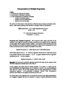
Assumptions in Multiple Regression: A Tutorial Statistical tests rely upon certain assumptions about the variables used in an analysis (Osborne & Waters, 2002). Since Cohen’s 1968 seminal article, multiple regression has become increasingly popular in both basic and applied research journals (Hoyt, Leierer, & Millington, 2006). It has been noted in the research that multiple regression (MR) is currently a major form of data analysis in child and adolescent psychology (Jaccard, Guilamo-Ramos, Johansson, & Bouris, 2006). Multiple regression examines the relationship between a single outcome measure and several predictor or independent variables (Jaccard et al., 2006). The correct use of the multiple regression model requires that several critical assumptions be satisfied in order to apply the model and establish validity (Poole & O’Farrell, 1971). Inferences and generalizations about the theory are only valid if the assumptions in an analysis have been tested and fulfilled. The use of MR has become common across a wide variety of social science disciplines including applied psychology and education specifically in the search of interaction effects and evaluating moderating effects of variables in theory development (Aguinis, Petersen, & Pierce, 1999; Mason & Perreault Jr., 1991; Shieh, 2010). Applications of MR in psychology often are used to test a theory about causal influences on the outcome measure (Jaccard et al., 2006). Multiple regression is attractive to researchers given its flexibility (Hoyt et al., 2006). MR can be used to test hypothesis of linear associations among variables, to examine associations among pairs of variables while controlling for potential confounds, and to test complex associations among multiple variables (Hoyt et al., 2006). The purpose of this tutorial is to clarify the primary assumptions and related statistical issues, and provide a basic guide for conducting and interpreting tests of assumptions in the multiple regression model of data analysis. It is assumed that the reader is familiar with the

ASSUMPTIONS IN MULTIPLE REGRESSION

3

basics of statistics and multiple regression which provide the framework for developing a deeper understanding for analysing assumptions in MR. Treatment of assumption violations will not be addressed within the scope of this paper. Statistical Issues and Importance Regression analyses are usually driven by a theoretical or conceptual model that can be drawn in the form of a path diagram (Jaccard et al., 2006). The path diagram provides the model for setting the regression and what statistics to examine (Jaccard et al., 2006). If one assumes linear relations between variables, it provides a ‘road map’ to a set of theoretically guided linear equations that can be analyzed by multiple regression methods (Jaccard et al., 2006). Multiple regression is widely used to estimate the size and significance of the effects of a number of independent variables on a dependent variable (Neale, Eaves, Kendler, Heath, & Kessler, 1994). Before a complete regression analysis can be performed, the assumptions concerning the original data must be made (Sevier, 1957). Ignoring the regression assumptions contribute to wrong validity estimates (Antonakis, & Deitz, 2011). When the assumptions are not met, the results may result in Type I or Type II errors, or over- or under-estimation of significance of effect size (Osborne & Waters, 2002). Meaningful data analysis relies on the researcher’s understanding and testing of the assumptions and the consequences of violations. The extant research suggests that few articles are reporting having tested the assumptions of the statistical tests they rely on for drawing their conclusions (Antonakis & Dietz, 2011; Osborne & Waters, 2002; Poole & O’Farrell, 1971). Sevier (1957) raised this concern many years ago, and it appears to continue to be an issue today. The result is that the rich literature in social sciences and education may have questionable results, conclusions, and assertions (Osborne & Waters,

ASSUMPTIONS IN MULTIPLE REGRESSION

4

2002). The validation and reliability of theory and future research relies on diligence in meeting assumptions of MR. Assumption Analysis The assumptions of MR that are identified as primary concern in the research include linearity, independence of errors, homoscedasticity, normality, and collinearity. This section will specifically define each assumption, review consequences of assumption failure, and address how to test for each assumption, and the interpretation of results. Linearity Some researchers argue that this assumption is the most important, as it directly relates to the bias of the results of the whole analysis (Keith, 2006). Linearity defines the dependent variable as a linear function of the predictor (independent) variables (Darlington, 1968). Multiple regression can accurately estimate the relationship between dependent and independent variables when the relationship is linear in nature (Osborne & Waters, 2002). The chance of non-linear relationships is high in the social sciences, therefore it is essential to examine analyses for linearity (Osborne & Waters, 2002). If linearity is violated all the estimates of the regression including regression coefficients, standard errors, and tests of statistical significance may be biased (Keith, 2006). If the relationship between the dependent and independent variables is not linear, the results of the regression analysis will under- or over- estimate the true relationship and increase the risk of Type I and Type II errors (Osborne & Waters, 2002). When bias occurs it is likely that it does not reproduce the true population values (Keith, 2006). Violation of this assumption threatens the meaning of the parameters estimated in the analysis (Keith, 2006).

ASSUMPTIONS IN MULTIPLE REGRESSION

5

One method of preventing non-linearity is to use theory of previous research to inform the current analysis to assist in choosing the appropriate variables (Osborne & Waters, 2002). Keith (2006) suggests that if you have reason to suspect a curvilinear relationship that you add a curve component (variable2) to the regression equation to see if it increases the explained variance. However, this approach may not be sufficient alone to detect non-linearity. More indepth examination of the residual plots and scatter plots available in most statistical software packages will also indicate linear vs. curvilinear relationships (Keith, 2006; Osborne & Waters, 2002). Residual plots showing the standardized residuals vs. the predicted values and are very useful in detecting violations in linearity (Stevens, 2009). The residuals magnify the departures from linearity (Keith, 2006). If there is no departure from linearity you would expect to see a random scatter about the horizontal line. Any systematic pattern or clustering of the residuals suggests violation (Stevens, 2009). Figure 1 visually demonstrates both linear and curvilinear relationships. In addition, detecting curvilinearity can be seen after utilizing the nonlinear regression option in a statistical package (Osborne & Waters, 2002). The amount of shared variance (R2) can be seen in an F-test. The F-test is designed to test if two population variances are equal (by comparing the ratio of two variances). If the variances are equal, the ratio of the variances will be one. A significant F value indicates a departure from linearity (Sevier, 1957). Figure1. Scatterplots showing linear and curvilinear relationships with standardized residuals by predicted values.

Osborne & Waters, 2002

ASSUMPTIONS IN MULTIPLE REGRESSION

6

Independence of Errors Independence of errors refers to the assumption that errors are independent of one another, implying that subjects are responding independently (Stevens, 2009). The goal of research is often to accurately model the ‘real’ relationships in the population (Osborne & Waters, 2002). In educational and social science research it is often difficult to measure variables, which makes measurement error an area of particular concern (Osborne & Waters, 2002). When independence of errors is violated standard scores and significance tests will not be accurate and there is increased risk of Type I error (Keith, 2006; Stevens, 2009). When data are not drawn independently from the population, the result is a risk of violating the assumption that errors are independent (Keith, 2002). This means that violations of this assumption can underestimate standard errors, and label variables as statistically significant when they are not (Keith, 2006). In the case of MR, effect sizes of other variables can be over-estimated if the covariate is not reliably measured (Osborne & Waters, 2002). Essentially what occurs is that the full effect of the covariate is not removed (Osborne & Waters, 2002). Violation of this assumption therefore threatens the interpretations of the analysis (Keith, 2006). One way to diagnose violations of this assumption is through the graphing technique called boxplots in most statistical software programs (Keith, 2006). The boxplots of residuals show the median, high and low values, and possible outliers (Keith, 2006). Examining the variability of the boxplots allows the researcher to explore violations to independence of errors (Keith, 2006). Figure 2 shows a sample boxplot from the IBM SPSS Statistics software program (SPSS) with variables at similar levels that meet the independence of errors assumption.

ASSUMPTIONS IN MULTIPLE REGRESSION

7

Figure 2. Boxplot with variables at similar levels

Homoscedasticity The assumption of homoscedasticity refers to equal variance of errors across all levels of the independent variables (Osborne & Waters, 2002). This means that researchers assume that errors are spread out consistently between the variables (Keith, 2006). This is evident when the variance around the regression line is the same for all values of the predictor variable. When heteroscedasticity is marked it can lead to distortion of the findings and weaken the overall analysis and statistical power of the analysis, which result in an increased possibility of Type I error, erratic and untrustworthy F-test results, and erroneous conclusions (Aguinis et al., 1999; Osborne & Waters, 2002). Therefore the incorrect estimates of the variance lead to the statistical and inferential problems that may hinder theory development (Antonakis & Dietz, 2011). However, it is good to note that the regression is fairly robust to violation of this assumption (Keith, 2006). Homoscedasticity can be checked by visual examination of a plot of the standardized residuals by the regression standardized predicted value (Osborne & Waters, 2002). Specifically, statistical software scatterplots of residuals with independent variables are the method for examining this assumption (Keith, 2006). Ideally, residuals are randomly scattered around zero (the horizontal line) providing even distribution (Osborne & Waters, 2002). Heteroscedasticity is indicated when the scatter is not even; fan and butterfly shapes are common

ASSUMPTIONS IN MULTIPLE REGRESSION

8

patterns of violations. Figure 3 shows some examples homoscedasticity and heteroscedasticity seen in scatterplots. When the deviation is substantial more formal tests for heteroscedasticity should be performed, such as collapsing the predictive variables into equal categories and comparing the variance of the residuals (Keith, 2006; Osborne & Waters, 2002). The rule of thumb for this method is that the ratio of high to low variance less than ten is not problematic (Keith, 2006). Bartlett’s and Hartley’s tests have been identified in the research as flexible and powerful tests to assess homoscedasicity (Aguinis et al., 1999; Sevier, 1957). Figure 3. Homoscedasticity and heteroscedasticity examples

Osborne & Waters, 2002

Collinearity Collinearity (also called multicollinearity) refers to the assumption that the independent variables are uncorrelated (Darlington, 1968; Keith, 2006). The researcher is able to interpret regression coefficients as the effects of the independent variables on the dependent variables when collinearity is low (Keith, 2006; Poole & O’Farrell, 1971). This means that we can make inferences about the causes and effects of variables reliably. Multicollinearity occurs when several independent variables correlate at high levels with one another, or when one independent variable is a near linear combination of other independent variables (Keith, 2006). The more variables overlap (correlate) the less able researchers can separate the effects of variables. In MR the independent variables are allowed to be correlated to some degree (Cohen, 1968; Darlington, 1968; Hoyt et al., 2006; Neale et al., 1994). The regression is designed to allow for

ASSUMPTIONS IN MULTIPLE REGRESSION

9

this, and provides the proportions of the overlapping variance (Cohen, 2968). Ideally, independent variables are more highly correlated with the dependent variables than with other independent variables. If this assumption is not satisfied, autocorrelation is present (Poole & O’Farrell, 1971). Multicollinearity can result in misleading and unusual results, inflated standard errors, reduced power of the regression coefficients that create a need for larger sample sizes (Jaccard et al., 2006; Keith, 2006). Interpretations and conclusions based on the size of the regression coefficients, their standard errors, or associated t-tests may be misleading because of the confounding effects of collinearity (Mason & Perreault Jr., 1991). The result is that the researcher can underestimate the relevance of a predictor, the hypothesis testing of interaction effects is hampered, and the power for detecting the moderation relationship is reduced because of the intercorrelation of the predictor variables (Jaccard et al., 2006; Shieh, 2010). One way to prevent multicollinearity is to combine overlapping variables in the analysis, and avoid including multiple measures of the same construct in a regression (Keith, 2006). Statistical software packages include collinearity diagnostics that measure the degree to which each variable is independent of other independent variables. The effect of a given level of collinearity can be evaluated in conjunction with the other factors of sample size, R2, and magnitude of the coefficients (Mason & Perreault Jr., 1991). Widely used procedures examine the correlation matrix of the predictor variables, computing the coefficients of determination, R2, and measures of the eigenvalues of the data matrix including variance inflation factors (VIF) (Mason & Perreault Jr., 1991). Tolerance measures the influence of one independent variable on all other independent variables. Tolerance levels for correlations range from zero (no independence) to one (completely independent) (Keith, 2006). The VIF is an index of the

ASSUMPTIONS IN MULTIPLE REGRESSION

10

amount that the variance of each regression coefficient is increased over that with uncorrelated independent variables (Keith, 2006). When a predictor variable has a strong linear association with other predictor variables, the associated VIF is large and is evidence of multicollinearity (Shieh, 2010). The rule of thumb for a large VIF value is ten (Keith, 2006; Shieh, 2010). Small values for tolerance and large VIF values show the presence of multicollinearity (Keith, 2006). Table 1 is an example of low collinearity demonstrated by high tolerance and low VIF values from the SPSS software. Table 1. Collinearity statistics Unstandardized

Standardized

Coefficients

Coefficients

Correlations

Collinearity Statistics

ZeroModel

B

1 (Constant) hours of math

Std. Error

7.640

6.705

1.532

.211

.208

.754

Beta

t

Sig.

order

Partial

Part

Tolerance

VIF

1.139

.256

.418

7.271

.000

.429

.421

.414

.985

1.016

.123

.101

1.696

.091

.053

.107

.097

.916

1.092

.382

.118

1.971

.050

.141

.125

.112

.903

1.108

homework per month teacher math support peer math support

Normality Multiple regression assumes that variables have normal distributions (Darlington, 1968; Osborne & Waters, 2002). This means that errors are normally distributed, and that a plot of the values of the residuals will approximate a normal curve (Keith, 2006). The assumption is based on the shape of normal distribution and gives the researcher knowledge about what values to expect (Keith, 2006). Once the sampling distribution of the mean is known, it is possible to make predictions for a new sample (Keith, 2006).

ASSUMPTIONS IN MULTIPLE REGRESSION

11

When scores on variables are skewed, correlations with other measures will be attenuated, and when the range of scores in the sample is restricted relative to the population correlations with scores on other variables will be attenuated (Hoyt et al., 2006). Non-normally distributed variables can distort relationships and significance tests (Osborne & Waters, 2002). Outliers can influence both Type I and Type II errors and the overall accuracy of results (Osborne & Waters, 2002). The researcher can test this assumption through several pieces of information: visual inspection of data plots, skew, kurtosis, and P-Plots (Osborne & Waters, 2002). Data cleaning can also be important in checking this assumption through the identification of outliers. Statistical software has tools designed for testing this assumption. Skewness and kurtosis can be checked in the statistic tables, and values that are close to zero indicate normal distribution. Normality can further be checked through histograms of the standardized residuals (Stevens, 2009). Histograms are bar graphs of the residuals with a superimposed normal curve that show distribution. The normal curve is fitted to the data using the observed mean and standard deviation as estimates, and computing the corresponding chi square (Sevier, 1957). Figure 4 is an example of is histogram with normal distribution from the SPSS software. Q-plots, and Pplots are a more exacting methods to spot deviations from normality, and are relatively easy to interpret as departures from a straight line (Keith, 2006). Figure 5 shows a P-Plot with normal distribution from the SPSS software.

ASSUMPTIONS IN MULTIPLE REGRESSION Figure 4. Histogram with normal distribution

12 Figure 5. Normal P-Plot

Conclusion Multiple regression techniques give researchers flexibility to address a wide variety of research questions (Hoyt et al., 2006). Since the analyses are based upon certain definite conditions or assumptions, it is imperative that the assumptions be analyzed (Sevier, 1957). The goal of this tutorial was to raise awareness and understanding of the importance of testing assumptions in MR for understanding and conducting research. The primary assumptions reviewed included linearity, independence of errors, homoscedasticity, collinearity, and normality. When assumptions are violated accuracy and inferences from the analysis are affected (Antonakis & Dietz, 2011). Statistical software packages allow researchers to test for each assumption. Checking the assumptions carry significant benefits for the researcher, reduce error, and increase reliability and validity of inferences. Consideration of the issues surrounding the assumptions in multiple regression should improve the insights for researchers as they build theories (Jaccard et al., 2006).

ASSUMPTIONS IN MULTIPLE REGRESSION

13

References Aguinis, H., Petersen, S., & Pierce, C. (1999). Appraisal of the homogeneity of error variance assumption and alternatives to multiple regression for estimating moderating effects of categorical variables. Organizational Research Methods, 2, 315-339. doi: 10.1177/109442819924001 Antonakis, J., & Dietz, J. (2011). Looking for validity or testing it? The perils of stepwise regression, extreme-score analysis, heteroscedasticity, and measurement error. Personality and Individual Differences, 50, 409-415. doi:10.1016/j.paid.2010.09.014 Cohen, J. (1968). Multiple regression as a general data-analytic system. Psychological Bulletin, 70(6), 426-443. Darlington, R. (1968). Multiple regression in psychological research and practice. Psychological Bulletin, 69(3), 161-182. Hoyt, W., Leierer, S., & Millington, M. (2006). Analysis and interpretation of findings using multiple regression techniques. Rehabilitation Counseling Bulletin, 49(4), 223-233. Jaccard, J., Guilamo-Ramos, V., Johansson, M., & Bouris, A. (2006). Multiple regression analyses in clinical child and adolescent psychology. Journal of Clinical Child and Adolescent Psychology, 35(3), 456-479. Keith, T. (2006). Multiple regression and beyond. PEARSON Allyn & Bacon. Mason, C., & Perreault Jr., W. (1991). Collinearity, power, and interpretation of multiple regression analysis. Journal of Marketing Research, 28(3), 268-280. Retrieved from: http://www.jstor.org/stable/3172863

ASSUMPTIONS IN MULTIPLE REGRESSION

14

Neale, M., Eaves, L., Kendler, K., Heath, A., & Kessler, R (1994). Multiple regression with data collected from relatives: Testing assumptions of the model. Multivariate Behavioral Research, 29(1), 33-61. Osborne, J., & Waters, E. (2002). Four assumptions of multiple regression that researchers should always test. Practical Assessment, Research & Evaluation, 8(2). Retrieved from: http://PAREonline.net/getvn.asp?v=8&n=2 Poole, M., & O’Farrell, P. (1971). The assumptions of the linear regression model. Transactions of the Institute of British Geographers, 52, 145-158. Retrieved from: http://www.jstor.org/stable/621706 Sevier, F. (1957). Testing assumptions underlying multiple regression. The Journal of Experimental Education, 25(4), 323-330. Retrieved from: http://www.jstor.org/stable/20154054 Shieh, G. (2010). On the misconception of multicollinearity in detection of moderating effects: Multicollinearity is not always detrimental. Multivariate Behavioral Research, 45, 483507. doi: 10.1080/00273171.2010.483393 Stevens, J. P. (2009). Applied multivariate statistics for the social sciences (5th ed.). New York, NY: Routledge.