tuar(Yr)Var(Yr-k). 0 fork> 1. (13.33). So, if we have an MA(q) model we will expect the correlogram (the graph of the. ACF) to have q spikes for k = q, and then go ...
.. .
! :. j
!
l
' J~~ · , . :~ •,··'-. .. .~"""·•< •..
,.,1: .
;
.
.
.;· . .
•. r1
ll
[l (l
r.--1 !. i. I
I ' f"J 1 .. '
I
i-)
···I
, I
IL f
·'
fl .I :j
i 'i : J
:. J i ' i..J
;I ··.
'·
!j r l. 1.
ll lj fl
.I
'• rl
!. ·~
1
c
"I
I
!
)
I
lI
I
·LJ i I
.\
->
[]
*
[J
© Dimitrios Asteriou and Stephen G. Hall 2006, 2007
All rights reserved. No reproduction, copy or transmission of this publication may be made ·without written permission.
u
No paragraph of this publication may be reproduced, copied or transmitted save with written permission or in accordance with the provisions of the
Copyright, Designs and Patents Act 1988, or under the terms of any licence permitting limited copying issued by the Copyright licensing Agency, 90 Tottenham Court Road, london WlT 4LP.
lj
Any person who does any unauthorised act in relation to this publication · may be liable to criminal prosecution and civil claims for damages. The authors have asserted their rights to be identified as the authors of this work in accordance with the Copyright, Designs and Patents Act 1988.
t·J
First edition 2006 Revised edition 2007 Published by PALGRAVE MACMILLAN Houndmills, Basingstoke, Hampshire RG21 6XS and 175 Fifth Avenue, New York, N.Y. 10010 Companies and representatives throughout the world.
[ '1
[l ll
PALGRAVE MACMILLAN is the global academic imprint of the Palgrave Macmillan division of St. Martin's Press, lLC and of Palgrave Macmillan ltd. Macmillan® is a registered trademark in the United States, United Kingdom and other countries. Palgrave is a registered trademark in the European Union and other countries. ISBN-13:978-0-230-50640-4 15BN-10: 0-230-50640-2 This book is printed on paper suitable for recycling and made from fully managed and sustained forest sources. A catalogue record for this book is available from the British library. A catalog record for this book is available from the library of Congress. 10 9 8 7 6 5 4 3 2 16 15 14 13 12 11 10 09 08 07
[_
Printed and bound in China
r·
! !.; '•
L '- [ j
..
~ .......
~-
~
1 ;-) I
l' ..
•I
l'
I'·
•'
[-
l_j
To Athina, for all her love and encouragement- D.A. To Jacquie, for al~ her help and understanding- S.G.H.
I-~
[j
.,
[J Ij
(,
ll [J 1
r
(
)
rl
1 J
I,
l1 [ j
[··:: [, ~
I:)
• J
11 l
[. l
r '
'
~ '
1.·_ i I.. ''
I-: I
··-'
r·'
i[,.::
l'vlar ~0 11
I
l_J
L~
~--·
-~
!
:;i-i
Contents
l __ :
Ii L:J
•,
I '
lJ
l I
l
List of Figures
xvii
List of Tables
xix
Preface
xxiii
Acknowledgements 1
I ,
l
~--
i
Introduction What is econometrics? The stages of applied econometric work
5
2
The Structure of Economic Data Cross-sectional data Time series data Panel data
7 8 8 9
3
Wor~ing
with Data: Basic Data Handling Looking at raw data Graphical analysis Graphs in MFit Graphs in EViews Summary statistics Summary statistics in MFit Summary statistics in EViews Components of a time series Indices and base dates Splicing two indices and changing the base date of an index Data transformations Changing the frequency of time series data Nominal versus real data Logs Differencing Growth rates
[ vii
r< r··
1
2 2
Part I' Statistical Background and Basic Data Handling i
I 1_,
XXV
11 I2 I2 I2 13 IS IS IS I6 16 16 17 17 17 18 18 19
l.~
.L -·1
l
·'
~ --~
.i r_.J
c- . ]
;
viii
Contents
Part II The Classical Linear Regression Model 4
5
Simple Regression Introduction to regression: the classical linear regression model (CLRM) Why do we do regressions? The classical linear regression model The ordinary least squares (OLS) method of estimation Alternative expressions for jj The assumptions of the CLRM General The assumptions Violations of the assumptions Properties of the OLS estimators Linearity Unbiasedness Efficiency and BLUEness Consistency The overall goodness of fit Problems associated with R 2 Hypothesis testing and confidence intervals Testing the significance of the OLS coefficients Confidence intervals How to estimate a simple regression in Microfit and EViews Simple regression in Microfit Simple regression in EViews Reading the EViews simple regression results output Presentation of regression results Applications Application 1: the demand function Application 2: a production function Application 3: Okun's law Application 4: the Keynesian consumption function Computer example: the Keynesian consumption function Solution Questions and exercises Multiple Regression Derivation of the multiple regression coefficients The three-variable model The k-variables case Derivation of the coefficients with matrix algebra The structure of the X')( and X'Y matrices The assumptions of the multiple regression model The variance-covariance matrix of the errors Properties of the multiple regression model OLS estimators Linearity Unbiasedness Consistency BLUEness
. tl
21
.I
23 24 24 24 26 28 29 29 30 31 31 32 33 34 36 37 38 39 40 41 42 42 42 43 44 44 44 45 46 46 47 47 52 56 57 57 58 59 60 61 62 62 62 63 63 63
' ll'-'
l ll
J
[]
l
f
j
I
t-l
L,
'•
j< \
' L;
L
I •
·'
--, r.,' r-·,
!. :
!, ; r·~~
I
~
l
[':
Contents R2 and adjusted R2 General criteria for model selection Multiple regression estimation in Microfit and £Views Multiple regression in Microfit Multiple regression in £Views Reading the £Views multiple regression results output Hypothesis testing. Testing individual coefficients Testing linear restrictions The F-form of the likelihood ratio test Testing the joint significance of theXs F-test for overall significance in Microfit and £Views Adding or deleting explanatory variables Omitted and redundant variables test in £Views Omitted and redundant variables test in Microfit How to perform the Wald test in EViews and Microfit The t test (A special case of the Wald procedure) The LM test The LM test in Microfit and £Views Computer example: Wald, omitted and redundant variables tests A Wald test of coefficient restrictions A redundant variable test An omitted variable test Questions and exercises
1---l L.J
r·;l
.,
L_-'
u
u l
f
u [·j [:'J
lJ
Part III '6
[ '1
p l
J
r:, r. i ' J ;
i
i
t
i
t' r
.
l· [ ·.! 'j
f·
ix
7
Violating the Assumptions of the CLRM
Multicollinearity Perfect multicollinearity Consequences of perfect multicollinearity Imperfect multicollinearity Consequences of imperfect multicollinearity Detecting problematic multicollinearity Simple correlation coefficient Rz from auxiliary regressions Corvputer examples Example 1: induced multicollinearity Example 2: with the use of real economic data Questions. and exercises Heteroskedasticity Introduction: what is heteroskedasticity? Consequences of heteroskedasticity on OLS estimators A general approach A mathematical approach Detecting heteroskedasticity The informal way The Breusch-Pagan LM test
65 66
67 67 67 68 68 68 68 70 71 71 72 72
73 73 74 74
75 75 76 77
78 79
83 85
86 87 88 89 91 91 91
92 92 94 97 100
101 103 103 104 107 107
108
l_
'l:
lJ ~[J Contents
X
The Glesjer LM test The Harvey-Godfrey LM test The Park LM test The Goldfeld-Quandt test # White's test Computer example: heteroskedasticity tests The Breusch-Pagan test The Glesjer test The Harvey-Godfrey test The Park test The Goldfeld-Quandt test The White test Engle's ARCH test Computer example of the ARCH-LM test Resolving heteroskedasticity Generalized (or weighted) least squares Computer example: resolving heteroskedasticity Questions and exercises 8
9
Autocorrelation Introduction: what is autocorrelation? What causes autocorrelation? First and higher order autocorrelation Consequences of autocorrelation on the OLS estimators A general approach A more mathematical approach Detecting autocorrelation The graphical method Example: detecting autocorrelation using the graphical method The Durbin-Watson test Computer example of the DW test The Breusch-Godfrey LM test for serial correlation Computer example of the Breusch-Godfrey test Durbin's h test in the presence of lagged dependent variables Computer example of Durbin's h test Resolving autocorrelation When p is known Computer example of the generalized differencing approach When p is unknown Computer example of the iterative procedure Questions and exercises Appendix Misspecification: Wrong Regressors, Measurement Errors and Wrong Functional Forms Omitting influential or including non-influential explanatory variables Consequences of omitting influential variables Including a non-influential variable
[_-]
111 112 113 114 116
Ii LI
117 117
I
I
l.J
120 120 121 121 123 124 126 126 127 129 131
Ll [:1 [. j
133 13~
134 135 136 136
-!
137
[ '
·I.
139
139 139 140 143 143 145 145 147 148 149 151 151 153 154 155
r·!
I~
'•
l..
i
156
157 157 158
L
i!! i
'
gl
I
f-~ l .•
'
I
f.:[. •'
r---
I
l_~
L:
Contents
I·'
Omission and inclusion· of relevant and irrelevant variables at the same time The plug-in solution in the omitted variable bias Various functional forms Introduction Linear-log functional form Reciprocal functional form Polynomial functional form Functional form including interaction terms Log-linear functional form The double-log functional form The Box-Cox transformation Measurement errors Measurement error in the dependent variable Measurement error in the explanatory variable Tests for misspecification Normality of residuals The Ramsey RESET test for general misspecification Te~ts for non-nested models Example: the Box-Cox transformation in EViews Approaches in choosing an appropriate model The traditional view: average economic regression The Hendry 'general to specific approach' Exercises
.I I
•
l_J
[]
.,
•
I
~
LJ
-I
l_
j
u u f-j
[j
Part IV Topics in Econometrics
' 10 [, .I
J "l
r--.
l' ~
r
[
:
[..: [.'1 l' .;
r-
r··
xi
Dummy Varia:~1es Introduction: the nature of qualitative information The use of dummy variables Intercept dummy variables Slope dummy variables The combined effect of intercept and slope dummies Computer example of the use of dummy variables Using a constant dummy Using a slope dummy Using both dummies together Special cases of the use of dummy variables Using dummy variables with multiple categories Using more than one dummy variable Using seasonal dummy variables Computer example of dummy variables with multiple categories Application: the January effect in emerging stockmarkets Tests for structural stability The dummy variable approach The Chow test for structural stability Questions
159 159 161 161 161 162 162 163 164 164 165 166 167 167 169 169 171 173 174 177 177
178 179
181 183 184 185 185 187 188 189 190 190 191 192 192 194 195 196 198 201 201 201 202
l_.
L l ·1i ·i
-'-'
11
12
Dynamic Econometric Models Distributed lag models The Koyck transformation The Almon transformation Other models of lag structures Autoregressive models The partial adjustment model A computer example of the partial adjustment model The adaptive expectations model Tests of autocorrelation in autoregressive models Exercises
203 204 205 207 208 208 208 209 211 213 213
Simultaneous Equation Models Introduction: basic definitions Consequences of ignoring simultaneity The identification problem Basic definitions Conditions for identification Example of the identification procedure A second example: the macroeconomic model of a closed economy Estimation of simultaneous equation models Estimation of an exactly identified equation: the method of ind.irect least squares Estimation of an overidentified equation: the method of two-stage least squares Example: the IS-LM model
215 216 217 217 217 218 219 219 220
Part V 13
.-r'1_j
Contents
xii
Time Series Econometrics
ARIMA Models and the Box-Jenkins Methodology An introduction to time series econometrics ARIMA models Stationarity Autoregressive time series models The AR(1) model The AR (p) model Properties of the AR models Moving average models The MA(1) model The MA(q) model Invertibility in MA models Properties of the MA models ARMA models Integrated processes and the ARIMA models An integrated series ARIMA models Box-Jenkins model selection Identification
lJ
u
-·
lJ
lJ lJ lj
u
' 221 221 222
l-,1
r
227 229 230 230 231 231 231 233 235 236 236 236 237 238 239 239 239 240 240 241
...,
l'
I
I
·';
jl
. I
J
"-
[ j t J
[ :: ._,
';
[ .-~ .·•
"-
.
[.
l '- [ "
1' • •
I
I
L
Contents
~-
I ~; , __ J
., 14
[ tXt
=1
(4.48)
Next, we proceed by deriving an expression for the variance (that we need to minimize) of the~.
Var(~) = E [~ - E(~)
( ;
t
t
L.l
= E [L 8t Yt -
\
=E[L8tYt- L8tE(Yr)t
E (L 8t Yt)
(
= E [L 8t(Yt- E(Yt))t
II
In this expression we can use Yt =a+ fJXt
L
[ )
!
l
l
and E(Y1) =a+ fJXt to give:
Var(~) = E [L 81 (a+ tJXt + Ut -(a+ .BXr)t
r ·I
lj
+ Ut
(4.49)
..
2
= E (L8tut) 22 22 22 = E(c5 22 1 u 1 + 82 u 2 + 83 u3 + · · · + 8nu 11 + 2.5 1 o2 u 1 u 2 + 28 1 .s 3 u 1 u3 + ... ) =.5 1ZE (u 21 )
2 2 + 8 2ZE (liz)+ li 32 E(u 23 ) +···+onZE (lin) + 28 182 E(Lquz) + 28 1 o3 E(ulu3) + · · ·)
J
!'",'
Using assumptions 5 (Var(Ut) obtain that:
= a 2 ) and 6 (Cov(ut, u5 ) Var(p)
r.
=L
= E(UtUs) = 0 for all t
8fa2
(4.50)
f= s) we
(4.51)
I
I·
I
r: I·
We now need to choose 81 in the linear estimator (4.46) to be such as to minimize the variance (4.5 1) subject to the constraints (4.49), which ensure unbiasedness (with this then having a linear, unbiased minimum variance estimator). We formulate the Langrangean function: L= a
[. r
I (··:~
"J
2
L 8( - A1 (:L 8t) - AZ (L: litXt - 1)
(4.52)
where Al and AZ are Langrangean multipliers. Following the regular procedure, which is to take the first-order conditions (i.e. the partial derivatives of L with respect to 8t, A1 and AZ) and set them equa.l to zero; and after rearrangement and mathematical manipulations (we omit the mathematical details of the derivation because it is very lengthy and tedious, and because it does not use any
'
!·. .
--'
[:J 36
'l..~'
The Classical Linear Regression Model
of the assumptions of the model anyway) we obtain the optimal 8t as: (4.53)
ll
Therefore, we have that 8t = Zt of the OLS expression given by (4.34). So, substituting this into our linear estimator iJ we have:
II\]
Xt
8t
= L.xf
iJ = L8tYt
=
"LztYt
)J
= "Lzt(Yt- Y + Y)* = Llt(Yt- Y) + y Llt
l.l ll
= LZtYt = L.xt~t L.xt
=~
(4.54)
Thus, the ~ of the OLS is the BLUE.
!1
The advantage of the BLUEness condition is that it provides us with an expression for the variance by substituting the optimal lit given in (4.53) into (4.51) to give:
Var(iJ)
= Var(,8) = L L,xfa2
(__!.!._) L.xf 2
2
1
l
(4.55)
2=a - -
(L.xf)
l. i
a2
L.xf
l
·; .,
':
Consistency Consistency is the idea that as the sample becomes infinitely large the parameter estimate given by a procedure such as OLS converges on the true parameter value. This is obviously true when the estimator is unbiased, as shown above, as consistency is really just a weaker form of unbiasedness. However the proof above rests on our assumption 3 that the X variables are fixed. If we relax this assumption then it is no longer possible to prove the unbiasedness of OLS but we can still establish that it is a consistent estimator. So when we relax assumption 3 OLS is no longer a BLU estimator but it is still consistent. We showed in equation (4.31) that~ = {3 + Cov(X, u)fVar(X), dividing the top and the bottom of the last term by n gives
.8 = f3 +
Cov(X,u)fn Var(X)/n
[.!
ll j ;:
'•
1··,
(4.56)
*We add and subtract Y.
I •~
.-?"
~,
L ,.
.
,
37
Simple Regression
[.
Using the law of large numbers·, we know that Cov(X, u)jn converges to its expectation which is Cov(Xt, Ut). Similarly, Var(X)jn converges to Var(Xt). So, as 11 --* oo; p--* f3 + Cov(Xt, u 1 )jVar(Xt), which is equal to the true population parameter f3 if Cov(Xt, Ut) = 0 (i.e. if X 1 and Ut are uncorrelated). Thus pis a consistent estimator of the true population .. · parameter {J.
C-
l~
I
c.,.j t,
I
i
!--" _
The overall goodness of fit
_})
!J I
We showed before that the regression equation obtained from the OLS method fits a scatter diagram quite closely. However, we need to know how close it is to the scattered observed values to be able to judge whether a particular line describes the relationship among Yt and Xt better than ari alternative line. In other words, it is desirable to know a measure which describes the closeness of fit. This measure will also inform us about how well the obtained equation accounts for the behaviour of the dependent variable. In order to obtain such a measure, we first have to decompose the actual value of Yt into a predicted value, which comes from the regression equation Yt plus the equation's residuals: Yt
= Yt + Ut
(4.57)
= Yt
(4.58)
subtracting Y from both sides we have: Yt - y
- y + itt
1)
I, \
We need to obtain a measure of the total variation in Y1 from its mean we take the sum of equation (4.58): L:lutlst;,..._,.., following steps should be iu, ulved:
J
Wf' "'"
"''"' (>
.. ,LdllU:.
ill
\l lJ
conduct general the
(0·
Step 1 Set the null and alternative hypothesis. It can be either Ho: f3 = 0; Ha: f3 ,;. 0 (two-tailed test), or if there is prior knowledge about the sign of the estimated coefficient (let's assume positive), H 0 : f3 = 0; Ha: f3 > 0 (one-tail test). Step 2
.l
11
Calculate the t-statistic by t = ((3- {3)/Sfi, where here because f3 u'nder null is equal to zero it becomes (3;sjJ (note that this is the t-statistic that• is automatically provided by EViews and Microfit in their starldard regression outputs).
Step 3
Find from the t-tables the t-critical for n- 2 degrees of freedom.
Step 4
If /lstati > itcrit I reject the null hypothesis.
I '( '
.I
.,i
Note that if we want to test a different hypothesis (i.e. that f3 = 1), then we need to change our null and alternative hypothesis in step 1 and calculate manually the t-statistic by the t = ((3 - {3)/SjJ formula. In this case it is not appropriate to use the t-statistic which is provided by EViews and Microfi.t.
l·
A rule of thumb of significance tests
The procedure for hypothesis testing outlined above presupposes that the researcher selects a significance level and then compares the value of the t -statistic with the critical value for this level. Several rules of thumb based on this approach have been developed, and these are useful in the sense that we do not need to consult statistical tables in cases of large samples (degrees of freedom >30). Note that the critical value for a So/o level of significance and for a very large sample (n- oo) reaches the value of ±1.96. For the same level and for 30 degrees of freedom it is ±2.045, while for 60 degrees of freedom it is exactly ±2.00. Therefore, for large samples it is quite safe to use as a rule of thumb a critical value of it/ > 2. For a one-tail test the rule of thumb changes with the t-value being It 1> 1.65. The rules stated above are nothing more that convenient approximations to these values. For 'small' samples we must use the specific values given in the t-table, as the above rules are not safe to apply.
r
!'
'•
\
,, r. - ~ ··-· r ..•
J
L ,?.!.·f.'-.~
_,._,
\
Il
'
r""
•:--
""'T
··iJY
·
i
I: 5i
Simple Regression
[' i
Table 4.6
~J
Dependent variable is Y
u~
20 observations used for estimation from 1 to 20
•,
u
c R-Squared S.E. of regression Mean of dependent variable Residual sum of squares Akaike info. criterion
u u u
I
2.3024 [.033) 15.7295 [.000)
R-bar-squared F-stat. F(1,18) S.D. of dependent variable
0.92841 247.4176 (.000)
Equation log-likelihood Schwarz bayesian criterion
-65.8964 -68.8921
25.7129
2.2838
LMVersion
A: Serial Correlation B: Functional Form C: Normality D: Heteroscedasticity
CHSQ(1) = 0.72444 CHSQ(1)=0.19091 CHSQ(2) = 0.35743 CHSQ(1) = 0.40046
F Version
[0.395) (0.662) [0.836) [0.527)
F(1, 17) = 0.63891 (.435) F(1,17)=0.16384(.691) Not applicable F(1, 18) =0.36778 (.552]
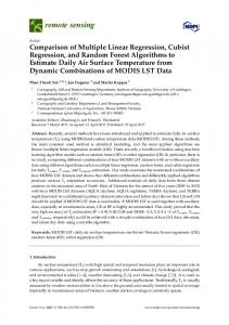
(. Table 4.7
EViews results from a simple regression model
Dependent Variable: Y Method: Le~st Squares Date: 01109104 Time: 16:13 Sample: 1-20 Included observations: 20 Variable
Coefficient
Std. Error
t-Statistic
c
15.11641 0.610889
6.565638 0.038837
2.302352 15.72951
X
1.
6.5656 0.038837
A Lagrat;~ge multiplier test of residual serial correlation. B Ramsey's RESET test using the square of the fitted values. C Based on a test of skewness and kurtosis of residuals. D Based on the regression of squared residuals on squared fitted values.
E
~
851.9210 -67.8964
T-Ratio[Prob]
Test Statistics
(I
r.
115.5160
Standard Error
Diagnostic Tests
' J
[.
0.93218 6.8796
OW-statistic
r -~
.
15.1164 0.61089
X
i
[.
Coefficient
Regressor
•. I
l1
Microfit Results from a Simple Regression Model
R·squared Adjusted R-squared S.E. of regression · Sum squared resid Log likelihood Durbin-Watson stat
0.932182 0.928415 6.879603 851.9210 -65.89639 2.283770
Mean dependent var S.D.dependentvar Akaike info criterion Schwarz criterion F -statistic Prob( F -statistic)
Prob.
0.0335 0.0000 115.5160 25.71292 6.789639 6.889212 247.4176 0.000000
6 After entering the data into EViews, the regression line (to obtain alpha and beta) can be estimated either by writing:
ls y c x (press enter)
I··_.
e~ lc:J
r--,
.j •.:
u The Classical Linear Regression Model
52
tJ
on the EViews command line, or by clicking on Quick/Estimate equation and then writing the equation {i.e. y c x) in the new window. Note that the option for OLS (LS - Least Squares (NLS and ARMA)) is automatically chosen by EViews and the sample is automatically chosen to be from 1 to 20. Either way the output shown in Table 4. 7 is shown in a new window which provides estimates for alpha (the coefficient of the constant term) and beta (the coefficient of X).
u u \ I
.J
i;
e~.~; ~;.t~~ ti· ~~!t ~/~· ~~-~~ ::·:_;•.;~:~·);, :;;~~ ~~r.\~. .
u u u
Questions 1 An outlier is :m observation that is very far from the sample regression function.
Suppose the equation is initially estimated using all observations and t~en reestimated omitting outliers. How will the estimated slope coefficient change? How will R2 change? Explain. 2 Regression equations are sometimes estimated using an explanatory variable that is a deviation from some value of interest. An example is a capacity utilization rateunemployment rate equation, such as: Ut
= ao + a1 (CAPt
j
\ '
-CAP[)+ er
ll
where CAP~ is a single value representing the capacity utilization rate corresponding to full employment (the value of 87.5% is sometimes used for this value).
.,
'
:
..·.:
(a) Will the estimated intercept from this equation differ from that in the equation with only CAPt as an explanatory variable? Explain.
\ .'
(b) Will the estimated slope coefficient from this equation differ from that in the
equation with only CAPt as an explanatory variable? Explain.
\. .·~.
3 Prove that the OLS coefficient for the slope parameter in the simple linear regression model is unbiased. 4 Prove that the OLS coefficient for the slope parameter in the simple linear regression model is BLUE.
f.
5 State the assumptions of the simple linear regression model and explain why they are necessary. '
Exercise 4.1
.
[ {
The following data refer to the quantity sold for a good Y (measured in kg), and the price of that good X (measured in pence per kg), for 10 different market locations: Y: X:
198 23
181 24.5
170 24
179 27.2
163 27
145 24.4
167 24.7
203 22.1
251 21
147 25
I·
I l. t"- -
•
~
.j
,-, ~
~;,~~
w...~-:'-~1-:f~(·""' ~
•
I
I I I_ . .
I
I~
Simple Regression
53
(~
I I (a) Assuming a linear relationship among the two variables, obtain the OLS estimators of a and {3. ~~,
(b) On a scatter diagram of the data, draw in your OLS sample regression·line.
! '
I,.J
•,
\...,'-
(c) Estimate the elasticity of demand for this good at the point of sample means (i.e. when Y = Y and X = X).
Exercise 4.2 The table below shows the average growth rates of GDP and employment for 25 OECD countries for the period 1988-97. I
)
r i. J
1
(I 1: 1'.
I,
i
~
rI .I'
lJ
(a) (
!
~
I
i.;
[
Ass~ming
Countries
Empl.
GDP
Countries
Empl.
GDP
Australia Austria Belgium Canada Denmark Finland France Germany Greece Iceland Ireland Italy japan
1.68 0.65 0.34 1.17 0.02 -1.06 0.28 0.08 0.87 -0.13 2.16 -0.30 1.06
3.04 2.55 2.16 2.03 2.02 1.78 2.08 2.71 2.08 1.54 6.40 1.68 2.81
Korea Luxembourg Netherlands New Zealand Norway Portugal Spain Sweden Switzerland Turkey United Kingdom United States
2.57 3.02 1.88 0.91 0.36 0.33 0.89 -0.94 0.79 2.02 0.66 1.53
7.73 5.64 2.86 2.01 2.98 2.79 2.60 1.17 1.15 4.18 1.97 2.46
a linear relationship obtain the OLS estimators.
(b) Provide an interpretation of the coefficients.
Exercise 4.3 In the Keynesian consumption function: d
r·
Ct=a+8Yt
the estimated marginal propensity to consume is simply 8 while the average propensity to consume is c;yd = a;Yd +8. Using data from 200 UK households on annual income and consumption (both of which were measured in UK£ ) we found the following regression equation:
f· r ,
! ("
.
I
[·
r
I.· I·
f ·:.
Ct
= 138.52 + 0.725Yf
R2
= 0.862
(a) Provide an interpretation of the constant in this equation and comment about its sign and magnitude. (b) Calculate the predicted consumption of a hypothetical household with annual income £40,000.
1-
,I
L :, I
\ 54
J. ·\
l
The Classical Linear Regression Model
(c) With
J
Y1 on the x-axis draw a graph of the estimated MPC and APC.
Exercise 4.4 Obtain annual data for the inflation rate and the unemployment rate of a country.
lJ
(a) Estimate the following regression which is known as the Phillips curve:
\ I~
~
.
rr1 = ao
J
+ a1 UNEMP 1 + u 1 \.
where rr 1 is inflation and UNEMP 1 is unemployment. Present the results in the usual way. (b) Estimate the alternative model: rr1 -rr1 _ 1
I
= a 0 + a 1 UNEMP 1 _ 1 + u1
1
I
I
'· J and calculate the NAIRU (i.e. when rr 1 -nr-1
= 0).
( !
(c) Reestimate the above equations splitting your sample into different decades. What factors account for differences in the results? Which period has the 'best-fitting' equation? State the criteria you have used. ·'
('"'\J
t"
[ ·,
Exercise 4.5
l' ~
The following equation has been estimated by OLS:
Rt = 0.567 + 1.045Rmt (0.33)
r
n = 250
(0.066)
\ l
where R 1 and Rmt denote the excess return of a stock and the excess return of the market index for the London Stock Exchange.
'• l.
(a) Derive a 95% confidence interval for each coefficient. (b) Are these coefficients statistically significant? Explain what is the meaning of your findings regarding the CAPM theory. (c) Test the hypothesis Ho: f3 = 1 and Ha: {3 < 1 at the 1% level of significance. If you reject Ho what does this indicate about this stock?
\ ~·
c
I
l
f..... ,
·- .....::.~,_;~.~--...:..;..~ i
L_ ~r";; = a 2 = constant for all t.
6 Cov(ur, u;) = E(ur, u;) = 0 for all j f:- t.
r I. ! ."
7 Each
lit
is normally distributed.
8 There are no exact linear relationships among the sample values of any two or more of the explanatory variables.
Il .
'j· '\ .,'·:. ·.
·I
'[
The Classical Linear Regression Model
·62
. '
The variance-covariance matrix of the errors
~
Recall from the matrix representation of the model that we have an 11 x 1 vector u of error terms. If we form an 11 x n matrix u'u and take the expected value of this matrix we get: E(uT) Ecu 2 u 1 ) E(uu')
E(u 1 u 2 ) E(u~)
E(l~~~t 1 ) £(1~~~2)
=
E(u 1 u3 ) E(u 2 u 3 )
.
...
E~~~)
···
£(1~~~1 11 )
E(u 11 u 3 )
...
E(u~)
t .. )
l )
E(u 11 u 1 )
E(u 11 uz)
a2
0
l
E(uu')
= (
0
0
(
0
0
...
2
In
1
[j
0
-~- .~. ~-~ . . . -~- = a 0
\1
0 0 ··· 0)
a2
.,
·i J
Now, since each error term, Ut, has a zero mean, the diagonal elements of ~his matrix will represent the variance of the disturbances, and the non-diagonal terms will be the covariances among the different disturbances. Hence, this matrix is called the variancecovariance matrix of the errors, and using assumptions 5 ( Var(llt) = Ez)
P=
f
tJ
J
ii, i'r, \\
::'..:-'' ·{j15z,.
.1)
.e variance-covariance ffidt' that from (5.32) we have:
substituting y = xp
.;J:
..
'
Which
•
.
,_.,..,fi,
,,,J71 . _ , , , .
Ll
EC/k -- ,\)::
i-'KJJ·,
(5.46)
'
f '·(
Var(A)
>)
iJ. We need to find an expression for
(X'X)- 1 )~ -.·
r·:\
(5.47)
·,
l'(
+ u, we get: {J = (X'X)- 1 X'(X{J + U)
=
(X'X)- 1 X'Xp
=
fJ
l-~ l
+ (X'X)- 1 X'u
+ (X'X)- 1 X'u
(5.48)
P- fJ = (X'X)- 1X'u
(5.49)
I
I
By the definition of variance-covariance we have that: Var(p)
(.,
= E[(p - fJ)(P - p)'] = E{[(X'X)- 1 X'u][(X'X)- 1 X'u]'J =
li
E[(X'X)- 1 X'uu'X(X'X)- 1 )*
..
= (X'X)- 1 X'E(uu')X(X'X)- 1t =
j.
(X'X)- 1 X'a 2 IX(X'X)- 1
= a 2 (X'X)- 1 *This is because (BA)' = A'B'. t This is because, by assumption 2, the Xs are non-random.
(5.50)
j• ::
jj
l ·. ,
65
Multiple Regression
~·~ ~ : I I ~~
Now for the BLUEness of the [1, let us assume that there is [1* which is any other linear estimator of {J, which can be expressed as:
~~
tJ
jJ*
•, ( i
I i
= [(X'X)- 1 X'
+ Z](Y)
where Z is a matrix of constants. Substituting for Y = X{J
~J
jJ*
= [(X'X)- 1 X'+ Z](X{J =
(5.5 1)
+ u, we get:
+ u)
p + ZX{J + (X'X)- 1 X'u + Zu
(5.52)
and for p"* to be unbiased we require that:
'-·,(·J \. 1
Using (5.53), we can rewrite (5.52) as:
lI . J
f.J
(5.53)
ZX=O
... )
jJ*- fJ
= (X'X)- 1 X'u
+ Zu
(5.54)
Going back to the definition of the variance-covariance:
.
E[(p-
fJ)(P- Pl'l = {(X'X)- 1 X'u + Zu}((X'X)- 1 X'u + Zu}' = u 2 (X'X)- 1
)1
+ u 2 ZZ'
(5.55) (5.56)
'
which says that the variance-covariance matrix of the alternative estimator p"* is equal to the variance-covariance matrix of the OLS estimator [1 plus u 2 times ZZ', and therefore .greater than the variance-covariance of [1. Hence [1 is BLUE.
R2
i
. I :~
..
.,
/.
,,
~.
( .
('· (
! I'
The regular coefficient of determination, R2 is again a measure of the closeness of fit in the mtiltiple regression model as in the simple two-variable model. However, R2 cannot be used as a means of comparing two different equations containing different numbers of explanatory variables. This is because when additional explanatory variables are included, the proportion of variation in Y explained by the Xs, R 2 , will always be increased. Therefore, we will always obtain a higher R 2 regardless of the importance or not of the additional regressor. For this reason we need a different measure that will take into account the number of explanatory variables included in each model. This measure is called the adjusted R2 (and is denoted by iF) because it is adjusted for the number of regressors (or adjusted for the degrees of freedom). · Recall that R 2 = ESSjTSS = 1 - RSS/TSS, so that the adjusted R 2 is just:
iF=
r (
and adiusted R2
j
1
_ RSSj(n- k) = _ RSS(n- 1) 1 TSSj(n- 1) TSS(n- k)
(5.57)
)_:
\'i,
tJ
The Classical Linear Regression Model
66
.iJ 'll..l
Thus, an increase in the number of Xs included in the regression function, increases k and this will reduce RSS (which if we do not adjust will increase Rz). Dividing now, RSS by n - k, the increase in k tends to offset the fall in RSS and this is why f?.2 is a 'fairer' measure in comparing different equations. The criterion of selecting a model is to include an extra variable only if it increases k 2 . Note that because (n- 1)/(11- k) is never less than 1, k 2 will never be higher than R2 . However, while R2 has values between 0 and 1 only, and can never be negative, k 2 can have a negative value in some cases. A negative k 2 indicates that the model does not adequately describe the data-generating process.
u
General criteria for model selection
t~ I
We said before that : > ••..•..>Jillg the n,,,, 'JE" ot explanatory variables in a multiple · regression model will decrease tt: J