chapter we will focus on linear regression or relationships that are linear (a line)
rather than curvilinear (a curve) in nature. Let's begin with the example used in ...
Gamma regression: estimation and testing .... distribution is the Gamma
distribution, i.e. ... For known ν in Y ∼ Gamma(µ, ν) the log likelihood is given by l
(µ, ν, y) ...
g(µi) = ln(µi). We need distribution for Yi ≥ 0 with E(Yi) = µi and V ar(Yi) = σ2µ2 i .
Such a distribution is the Gamma distribution, i.e.. Y ∼ Gamma(ν, λ) with fY (y) ...
mod1
tuar(Yr)Var(Yr-k). 0 fork> 1. (13.33). So, if we have an MA(q) model we will expect the correlogram (the graph of the. ACF) to have q spikes for k = q, and then go ...
1.93))] Note: while this is the interpretation of the intercept, we are ... change in the response based on a 1-unit change in the corresponding explanatory variable ...
Sir Francis Galton (1885) introduced the idea of “regression” to the research ... to
produce the most accurate prediction estimates (see Montgomery & Peck,.
The listing for the multiple regression case suggests that the data are found in a
... Only a small minority of regression exercises end up by making a prediction,.
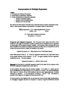
Multiple Linear Regression The population model • In a simple linear regression model, a single response measurement Y is related to a single
As an illustration, suppose we simulate random (standard normal) âpredictor ... 50. Residual. Latitude. A strong suggestion that the longitude effect is quadratic:.
University of Hertfordshire Business School .... the historical notes below. ..... Fitting linear relationships: A history of the calculus of observations 1750-1900.
It could have something to do with what part of the country they live in. .... correlations down so that you can figure out the value of multiple R. So, again, trying to ...
many of these topics will be covered again as we go through the semester.)
Those wanting more detail and worked examples should look at my course notes
for Grad Stats I. ..... example, bk = 2, sbk = 1, and the “critical” value for T is 1.96.
Multiple regression is a very advanced statistical too and it is extremely .... Figure 4-2 is a good illustration about what multiple correlation and regression is. Age.
Chapter 12. Architectural Drafting. Using AutoCAD. Copyright by Goodheart-
Willcox Co., Inc. Chapter 12 Exercises 1. E x E r C I s E s. Exercise 12-8. 1.
Continue ...
Chapter 20. Architectural Drafting. Using AutoCAD. Copyright by Goodheart-
Willcox Co., Inc. Chapter 20 Exercises. E x E r C I s E s. Exercise 20-8 . Continue
...
6.6 Special Considerations for Supervision of Exercising MS Patients . ...
pathophysiology of multiple sclerosis (MS) is characterised by fatigue,. Abstract
motor weakness ... therapy in the treatment of MS remains relatively ...
unexplored[7,8] c
is for water temperature to be between 80 and 86 degrees Fahrenheit. Aquatic Exercise and MS .... well as class programm
Katsuhisa Fujinaga, Mitsuru Nakai, Hiroshi Shimodaira and Shigeki Sagayama. Japan Advanced Institute of Science and Technology. Tatsu-no-Kuchi, Ishikawa, ...
[14] Azhar, N. and Farouqi, R. U. 2008. Cost Overrun Factors in the ... [20] Nasiru, Zakari Muhammad, Kunya Sani Usman, and Abdurrahman. Mutawakkil. 2012.
Nov 29, 2016 - aDepartment of Mathematics, University of Louisiana, Lafayette, LA, USA; bApplied ... Institute, Kolkata, India; cDepartment of Biostatistics and Epidemiology, Augusta University, Augusta, GA, USA ... ARTICLE HISTORY.
Jun 6, 2018 - Increasing use of machine learning in adversarial settings has motivated ...... Throughout, we abbreviate our proposed approach as MLSG, and ...
In Chapter 2, we learned how to use simple regression analysis to explain a
dependent variable ... the advantages of multiple regression over simple
regression.
These formulas are handy in stepwise regression procedures. Incidentally, R. 2 is biased upward, particularly in small samples. Therefore, adjusted R. 2 is.
Exercises. 8. MULTIPLE REGRESSION & MODEL SIMPLIFICATION. Model
Simplification. The principle of parsimony (Occam's razor) requires that the model
...
STATISTICS: AN INTRODUCTION USING R By M.J. Crawley Exercises
8. MULTIPLE REGRESSION & MODEL SIMPLIFICATION
Model Simplification The principle of parsimony (Occam’s razor) requires that the model should be as simple as possible. This means that the model should not contain any redundant parameters or factor levels. We achieve this by fitting a maximal model then simplifying it by following one or more of these steps: • • • • • •
remove non-significant interaction terms; remove non-significant quadratic or other non-linear terms; remove non-significant explanatory variables; group together factor levels that do not differ from one another; amalgamate explanatory variables that have similar parameter values; set non-significant slopes to zero within ANCOVA
subject, of course, to the caveats that the simplifications make good scientific sense, and do not lead to significant reductions in explanatory power. Model Saturated model
Maximal model
Minimal adequate model
Null model
Interpretation One parameter for every data point Fit: perfect Degrees of freedom: none Explanatory power of the model: none Contains all (p) factors, interactions and covariates that might be of any interest. Many of the model’s terms are likely to be insignificant Degrees of freedom: n - p – 1 Explanatory power of the model: it depends A simplified model with 0 ≤ p ′ ≤ p parameters Fit: less than the maximal model, but not significantly so Degrees of freedom: n – p’ – 1 Explanatory power of the model: r2 = SSR/SST Just 1 parameter, the overall mean y Fit: none; SSE = SST Degrees of freedom: n – 1 Explanatory power of the model: none
The steps involved in model simplification There are no hard and fast rules, but the procedure laid out below works well in practice. With large numbers of explanatory variables, and many interactions and non-linear terms, the process of model simplification can take a very long time. But this is time well spent because it reduces the risk of overlooking an important aspect of the data. It is important to realise that there is no guaranteed way of finding all the important structures in a complex data frame.
Step 1
2
3
4
5
Procedure Fit the maximal model
Explanation Fit all the factors, interactions and covariates of interest. Note the residual deviance. If you are using Poisson or binomial errors, check for overdispersion and rescale if necessary Begin model Inspect the parameter estimates using simplification summary. Remove the least significant terms first, using update -, starting with the highest order interactions Leave that term out of the model If the deletion causes an Inspect the parameter values again insignificant increase in Remove the least significant term remaining deviance Put the term back in the model using update If the deletion causes a + . These are the statistically significant significant increase in terms as assessed by deletion from the deviance maximal model Keep removing terms from Repeat steps 3 or 4 until the model contains the model nothing but significant terms This is the minimal adequate model If none of the parameters is significant, then the minimal adequate model is the null model
Deletion Deletion uses the update directive to remove terms from the model (you can automate this procedure, using step). Perhaps the simplest deletion is to remove the intercept from a regression study using the ~ . -1 directive (you need to be careful with the punctuation: the update formula contains “tilde dot minus” which means “fit the model (the tilde) with the last set of explanatory variables (the dot) but remove (the minus sign) the following”). This fits a new regression line with a single parameter Note that it does not rotate the regression line about the point ( x , y ) until it passes through the origin (a common misconception). We can demonstrate this as follows. Take the following data x