Jun 18, 2014 - framework of computations as shown recently by Lesch [12]. 5 .... A.S. acknowledges support of a grant from the John Templeton Foundation.
Asymmetric noncommutative torus 1∗ Ludwik Dabrowski ˛ and Andrzej Sitarz2,3
arXiv:1406.4645v1 [math.QA] 18 Jun 2014
1
SISSA (Scuola Internazionale Superiore di Studi Avanzati), via Bonomea 265, 34136 Trieste, Italy 2
3
Institute of Physics, Jagiellonian University, Reymonta 4, 30-059 Kraków, Poland
Institute of Mathematics of the Polish Academy of Sciences, ´ Sniadeckich 8, 00-656 Warszawa, Poland.
Abstract We compute the scalar curvature and prove the Gauss-Bonnet formula for a family of Dirac operators on a noncommutative torus, which are not (a priori) conformally related to "flat" Dirac operators.
1
Introduction
In the seminal works [2], [5] Connes and Tretkoff initiated the investigation of curvature aspects on the noncommutative two torus and have shown the analogue of Gauss-Bonnet theorem for the conformally rescaled Dirac D and the related spin Laplacian corresponding to the standard conformal structure. In [8] these studies were extended to arbitrary conformal structure. The scalar curvature itself was defined and computed in [4] and independently in [9]. The methods used in these papers build on Connes’ pseudodifferential calculus[5] and heat kernel small time asymptotic expansion. The novelty therein is the employment of twisted spectral triples, non-tracial weight and the modular operator. For some related papers see [1] [10], [11]. In [6] using the conformal (Weyl) factor from the commutant algebra and thus remaining on the level of the usual spectral triples, the Gauss-Bonnet has been established and the saclar curvture computed perturbatively up to the second order, for a wider class of Dirac operators. In the present paper we establish the Gauss-Bonnet and compute the scalar curvature nonperturbatively for the class of Dirac operators obtained by asymmetric rescaling of only a part of the standard Dirac operator. For that we employ a positive element which can belong to ∗
Partially supported by PRIN 2010 grant “Operator Algebras, Noncommutative Geometry and Applications"
the counterpart of coordinate algebra in the commutant, thus remaining on the level of usual spactral triples, or it can belong to the coordinate algebra itself, in which case however we are outside even of the class of twisted or modular spectral triples. These results are possible due to a very recent neat generalization by Lesch [12] of the "rearrangement lemma", which is an important technical tool in [5].
2
Dirac operator
Let T2 be the classical torus with coordinates 0 ≤ x, y ≤ 2π, equipped with the metric dx2 + k −2 (x, y)dy 2 ,
(2.1)
where k is a strictly positive function. The motivation for such a choice comes from the usual realization of T2 as an embedded surface in R3 : The "usual" symmetric torus has the following parametrization: X = (c + cos y) cos x,
Y = (c + cos y) sin x,
Z = sin y.
With the induced metric this is a particular case of the „asymmetric torus” corresponding to k −1 = c + cos y in (2.1).
Torus embedded in R3
Asymmetric torus in R3
The scalar curvature of the torus with the metric (2.1) reads R = 2k −1 ∂x2 (k) − 4k −2 (∂x (k))2 .
(2.2)
In the commutative case such metric is, of course, conformally equivalent to some flat metric on the torus even though the explicit formula for the curvature depends on the chosen coordinate system. However, when passing to the noncommutative torus we are entering a new unexplored land, where one does not know what is metric and what exactly means conformally equivalent. As in the approach of Connes the natural object is the Dirac operator rather than the metric itself, for this reason we propose a new Dirac operator, which generalizes to the noncommutative situation the classical case of asymmetric torus. We start with the commutative case of Dirac operator on L2 (T2 , k −1 dx dy) ⊗ C2 for the metric (2.1): � ˜ = −iσ 1 ∂x − 1 k −1 ∂x (k) − iσ 2 k ∂y , D 2 2
where
�
1
σ = Using the multiplication by
0 1
1 0
�
2
,
σ =
�
0 i
−i 0
� .
(2.3)
√
k we obtain the unitarily equivalent Dirac operator � ˜ = −iσ 1 ∂x − iσ 2 k ∂y + 1 ∂y (k) D 2
(2.4)
on L2 (T, dx dy) ⊗ C2 . It is selfadjoint on the dense domain H 1,2 (T ). Next we pass to the noncommutative torus T2θ , for which we refer to [3] for the needed information. As the Dirac operator we take D of the form (2.4), however, with −i times the partial derivatives replaced by the usual derivations on T2θ : � D = σ 1 δ1 + σ 2 k δ2 + 21 δ2 (k) (2.5) It acts on H = L2 (T2θ , t) ⊗ C2 , where t is the usual trace on T2θ . Such an operator is a differential operator in the sense of [5] and we can extract the associated scalar curvature following [5], [4].
3
The curvature
The square of D reads D2 = (δ1 )2 + k 2 (δ1 )2 + +
�
3 kδ2 (k) + 21 δ2 (k)k + iσ 3 δ1 (k) δ2 2 � 1 (δ (k))2 + 21 iσ 3 δ12 (k) + 12 kδ22 (k) . 4 2
�
and its symbol is σ(D2 ) = a0 + a1 + a2 , where
a0 = ξ12 + k 2 ξ22 a1 = a2 =
�
3 kδ2 (k) + 21 δ2 (k)k + iσ 3 δ1 (k) ξ2 2 � 1 (δ (k))2 + 21 iσ 3 δ12 (k) + 21 kδ22 (k) . 4 2
�
As was demonstrated first in [5] the value ζ(0) at the origin of the zeta function of the operator D2 is given by Z ζ(0) = − t(b2 (ξ)) dξ, where b2 (ξ) is a symbol of order −4 of the pseudodifferential operator (D2 + 1)−1 . It can be computed by pseudodifferential calculus of symbols from the symbol a2 (ξ) + a1 (ξ) + a0 (ξ) of D2 as follows: b2 = − (b0 a0 b0 + b1 a1 b0 + ∂1 (b0 )δ1 (a1 )b0 + ∂2 (b0 )δ2 (a1 )b0 + ∂1 (b1 )δ1 (a2 )b0 + ∂2 (b1 )δ2 (a2 )b0 + 21 ∂11 (b0 )δ12 (a2 )b0 + 21 ∂22 (b0 )δ22 (a2 )b0 + ∂12 (b0 )δ12 (a2 )b0 ), 3
(3.1)
where
b1 = −(b0 a1 b0 + ∂1 (b0 )δ1 (a2 )b0 + ∂2 (b0 )δ2 (a2 )b0 ), (3.2) b0 = (a2 + 1)−1 , Since to obtain the curvature (or the zero of the ζD2 function), we need to integrate with respect to ξ1 , ξ2 , we notice that terms which contain odd powers of these variables shall vanish. Therefore, we can neglect them and keep only the relevant parts for the computations with even powers. We have: be2 = A + B + C, where A = − 2kb20 δ1 (k)kb0 δ1 (k)b0 ξ24 + 4kb20 δ1 (k)kb20 δ1 (k)b0 ξ12 ξ24 − 2kb20 δ1 (k)b0 δ1 (k)kb0 ξ24 + 4kb20 δ1 (k)b20 δ1 (k)kb0 ξ12 ξ24 + 8kb30 δ1 (k)kb0 δ1 (k)b0 ξ12 ξ24 + 8kb30 δ1 (k)b0 δ1 (k)kb0 ξ12 ξ24 − b0 δ1 (k)b0 δ1 (k)b0 ξ22 + 2b20 δ1 (k)δ1 (k)b0 ξ22 − 2b20 δ1 (k)kb0 δ1 (k)kb0 ξ24 + 4b20 δ1 (k)kb20 δ1 (k)kb0 ξ12 ξ24 − 2b20 δ1 (k)k 2 b0 δ1 (k)b0 ξ24 + 4b20 δ1 (k)k 2 b20 δ1 (k)b0 ξ12 ξ24 − 8b30 δ1 (k)δ1 (k)b0 ξ12 ξ22 + 8b30 δ1 (k)kb0 δ1 (k)kb0 ξ12 ξ24 + 8b30 δ1 (k)k 2 b0 δ1 (k)b0 ξ12 ξ24 , kb0 δ2 (k)kb0 δ2 (k)b0 ξ22 − 3kb0 δ2 (k)k 2 b20 δ2 (k)kb0 ξ24 − 3kb0 δ2 (k)k 3 b20 δ2 (k)b0 ξ24 B = 15 4 + 49 kb0 δ2 (k)b0 δ2 (k)kb0 ξ22 + 6k 2 b20 δ2 (k)δ2 (k)b0 ξ22 − 8k 2 b20 δ2 (k)kb0 δ2 (k)kb0 ξ24 − 10k 2 b20 δ2 (k)k 2 b0 δ2 (k)b0 ξ24 + 4k 2 b20 δ2 (k)k 3 b20 δ2 (k)kb0 ξ26 + 4k 2 b20 δ2 (k)k 4 b20 δ2 (k)b0 ξ26 − 12k 3 b20 δ2 (k)kb0 δ2 (k)b0 ξ24 + 4k 3 b20 δ2 (k)k 2 b20 δ2 (k)kb0 ξ26 + 4k 3 b20 δ2 (k)k 3 b20 δ2 (k)b0 ξ26 − 10k 3 b20 δ2 (k)b0 δ2 (k)kb0 ξ24 − 8k 4 b30 δ2 (k)δ2 (k)b0 ξ24 + 8k 4 b30 δ2 (k)kb0 δ2 (k)kb0 ξ26 + 8k 4 b30 δ2 (k)k 2 b0 δ2 (k)b0 ξ26 + 8k 5 b30 δ2 (k)kb0 δ2 (k)b0 ξ26 + 8k 5 b30 δ2 (k)b0 δ2 (k)kb0 ξ26 − 41 b0 δ2 (k)δ2 (k)b0 + 43 b0 δ2 (k)kb0 δ2 (k)kb0 ξ22 + 45 b0 δ2 (k)k 2 b0 δ2 (k)b0 ξ22 − b0 δ2 (k)k 3 b20 δ2 (k)kb0 ξ24 − b0 δ2 (k)k 4 b20 δ2 (k)b0 ξ24 ;
and
C = + kb20 δ11 (k)b0 ξ22 − 4kb30 δ11 (k)b0 ξ12 ξ22 + b20 δ11 (k)kb0 ξ22 − 4b30 δ11 (k)kb0 ξ12 ξ22 − 21 kb0 δ22 (k)b0 + 2k 2 b20 δ22 (k)kb0 ξ22 + 4k 3 b20 δ22 (k)b0 ξ22 − 4k 4 b30 δ22 (k)kb0 ξ24 − 4k 5 b30 δ22 (k)b0 ξ24 , Similarly for the chiral part of the curvature: γ γ γ bγe 2 = A +B +C ,
where
Aγ = − 2k 2 b20 δ1 (k)kb0 δ2 (k)b0 iξ24 − 2k 2 b20 δ1 (k)b0 δ2 (k)kb0 iξ24 + 25 b0 δ1 (k)kb0 δ2 (k)b0 iξ22 − 2b0 δ1 (k)k 2 b20 δ2 (k)kb0 iξ24 − 2b0 δ1 (k)k 3 b20 δ2 (k)b0 iξ24 + 23 b0 δ1 (k)b0 δ2 (k)kb0 iξ22 B γ = 23 kb0 δ2 (k)b0 δ1 (k)b0 iξ22 − 2k 2 b20 δ2 (k)kb0 δ1 (k)b0 iξ24 − 2k 3 b20 δ2 (k)b0 δ1 (k)b0 iξ24 + 21 b0 δ2 (k)kb0 δ1 (k)b0 iξ22 ; 4
and C γ = 2k 2 b20 δ12 (k)b0 iξ22 − 21 b0 δ12 (k)b0 i,
3.1
The classical limit
At this point we can check the classical (commutative) value of our expressions for θ = 0. They become respectively: b2 =48b50 k 6 δ2 (k)2 ξ26 + 48b50 k 2 δ1 (k)2 ξ12 ξ24 − 8b40 k 5 δ22 (k)ξ24 − 56b40 k 4 δ2 (k)2 ξ24 − 8b40 k 2 δ1 (k)2 ξ24 − 8b40 kδ11 (k)ξ12 ξ22 − 8b40 δ1 (k)2 ξ12 ξ22 + 6b30 k 3 δ22 (k)ξ22 + 14b30 k 2 δ2 (k)2 ξ22 + 2b30 kδ11 (k)ξ22 + b30 δ1 (k)2 ξ22 − 1/2b20 kδ22 (k) − 1/4b20 δ2 (k)2 , and bγ2 = −12b40 k 3 δ1 (k)δ2 (k)iξ24 + 2b30 k 2 δ12 (k)iξ22 + 6b30 kδ1 (k)δ2 (k)iξ22 − 1/2b20 δ12 (k)i, which after integration gives: Z
and
π (δ1 (k))2 π δ11 (k) dξ1 dξ2 b2 = − + , 3 k3 6 k2 Z dξ1 dξ2 b2γ = 0.
Taking into account that we compute the Gilkey-Seeley-deWitt coefficients for the asymptotic heat kernel expansion of the square of the Dirac operator and not the Laplace operator itself, and assuming that D has no zero eigenvalue, we have: Z 1 √ gR. ζ(0) = 48π R Moreover, since t = 4π1 2 dx dy for θ = 0, taking into account the appropriate rescaling of the volume form and putting it all together we obtain: � � � 1 π (∂1 (k))2 π ∂11 (k) √ −2 −3 2 + = 2k ∂ (k) − 4k (∂ (k)) , gR = 48π 2 − 11 1 4π 3 k3 6 k2 which agrees with the classical formula (2.2). Similarly, √ gRγ = 0. Before we can proceed with the noncommutative computation let us recall the general framework of computations as shown recently by Lesch [12].
5
3.2
Rearrangement Lemma
In [12] Lesch proved the following formula: Z ∞ f0 (uk 2 )·b1 · f1 (uk 2 ) · b2 · · · bp · fp (uk 2 )du =
(3.3)
0
=k
−2
(1) (1) (2) (1) F (∆2 , ∆2 ∆2 , . . . , ∆2
where the function F (s1 , . . . , sp ) is Z F (s) =
(p) · · · ∆2 )(b1
· b2 · · · bp ),
∞
f0 (u)f1 (us1 ) · · · fp (usp )du
0 (j)
and ∆2 ; signifies the square of the modular operator ∆2 = ∆2 , acting on the j-th component of the produc. Here we shall rather use ∆ = k −1 · k instead of its square. In our case we need to adapt the formula to a slightly different setting, when we integrate over two variables ξ1 and ξ2 . A generic integral we have is of the form: Z
∞
J =
Z
∞ 2k1 2k2 n3 m3 2 dξ2 k n1 b0m1 (ξ1 , ξ2 ) X k n2 bm 0 (ξ1 , ξ2 ) Y k b0 (ξ1 , ξ2 )ξ1 ξ2 ,
dξ1 −∞
−∞
where X, Y are derivations of k and b0 (ξ1 , ξ2 ) =
1 . 1 + ξ12 + k 2 ξ 2
Extending the result of Lesch we see that J = F (∆(1) , ∆(1) ∆(2) )(X · Y ), where, after change of variables we obtain: Z F (s, t) = 2
∞
Z dv
0
1
∞
du k
n1 +n2 +n3−1−2k2
0
uk2 − 2 v 2k1 sn2 tn3 . (1 + v 2 + u)m1 (1 + v 2 + us2 )m2 (1 + v 2 + ut2 )m3
In case Y = 1 the resulting function depends only on s.
3.3
The curvature and its trace
In order to compute explicitly the expressions.for the curvature we shall use the following lemma. Lemma 3.1. Under the trace an entire function F of two variables satisfies � � t F (∆(1) , ∆(1) ∆(2) )(X · Y ) = t F (∆(1) , id (XY ) = t(F (∆(1) , 1)(X)Y ). and in case of one variable: � t F (∆(1) )(X) = t (F (1)X) . 6
Proof. We have: F (s, t) =
X
fnm sn tm ,
n,m≥0
so:
X � � t F (∆(1) , ∆(1) ∆(2) )(X · Y ) = fnm t ∆n+m (X)∆m (Y ) n,m≥0
=
X
fnm t (∆m (∆n (X)Y ))
n,m≥0
=
X
fnm t (∆n (X)Y )
n,m≥0
� = t F (∆(1) , 1)(X · Y ) . The other identity is a simple consequence of the above one.
3.4
Curvature and chiral curvature
We first compute the chiral curvature. Lemma 3.2. The chiral curvature for the asymmetric torus is: Rγ = G12 (δ1 (k), δ2 (k)) + G21 (δ2 (k), δ1 (k)) + G(δ12 (k)), where G12 (s, t) =
(t − 1) π , 2 k (t + 1)2 (s + 1)
G21 (s, t) =
π (t − 1) , 2 k (t + 1)2 (s + t)
and G(s) = −
π (s − 1) . k (s + 1)2
and its trace vanishes. Proof. By computation. Then the last statement follows from: G12 (s, 1) = G21 (s, 1) = G(1) = 0.
Next we compute the scalar curvature. Lemma 3.3. The scalar curvature for the asymmetric torus is: 0 0 R = F11 (δ1 (k), δ1 (k))+F11 (δ1 (k)2 )+F22 (δ2 (k), δ2 (k))+F22 (δ2 (k)2 )+F1 (δ11 (k))+F2 (δ22 (k)),
where F11 (s, t) = −
2π (2s2 + 4st + 4s + 3 + 8t + 3t2 ) , 3k 3 (t + 1)3 (s + 1)(s + t) 7
0 F11 (s) =
4π 1 , 3k 3 (s + 1)3
F22 (s, t) =
π (t2 − 6t + 1) , 2k (t + 1)3
F20 (s) = −
π (s2 − 6s + 1) , 2k (s + 1)3
and
1 2π . 2 3k (s + 1)2
F1 (s) =
F2 (s) = 0. and its trace vanishes. Proof. First of all, observe that 0 F22 (s, 1) + F22 (1) = 0,
F2 (1) = 0,
so all terms containing δ2 (k) and δ22 (k) vanish. For the terms containing δ1 (k) we have: 0 F11 (s, 1) + F11 (1) = −
π s+3 , 3k 3 (s + 1)2
then using the identity: � � � t k −2 δ11 (k) = 2t k −2 δ1 (k)k −1 δ1 (k) = 2t k −3 ∆−1 (δ1 (k))δ1 (k) , which follows directly from the Leibniz rule and the fact that the trace is closed, we can rewrite all the terms: � � 0 t F11 (δ1 (k), δ1 (k)) + F11 (δ1 (k)2 ) + F1 (δ11 (k)) = t k −3 H(∆)(δ1 (k))δ1 (k) , where H(s) =
π 1−s . 3k 3 s(s + 1)2
Next, we observe that for any A and B and an entire function H: � � � t k −3 H(∆)(A)B = t H(∆)(∆3 (A))k −3 B = t k −3 BH(∆)(∆3 (A)) , and � � t k −3 H(∆)(A)B = t k −3 AH(∆−1 )(B) . Now if A = B then both expressions on the right-hand side are identical. In our case, however: H(s)s3 =
π s2 (1 − s) , 3k 3 (s + 1)2 8
and H(s−1 ) =
π s2 (s − 1) , 3k 3 (s + 1)2
and therefore since H(s)s3 = −H(s−1 ), the trace of the above expression must vanish, hence, the Gauss-Bonnet theorem holds.
4
Conclusions
We have introduced a new class of Dirac operators on the noncommutative tori, computed the scalar curvature and shown that the Gauss-Bonnet theorem holds. Even though in the classical limit they arise from the metric, which is conformally equivalent to the flat one, this might not be the case in the noncommutative situation. This raises an intersting question how the metrics as defined above and the flat one are related to each other in the noncommutative case? Moreover, it becomes now more evident that the class of admissible Dirac operators on the noncommutative torus is certainly bigger than the one-parameter family of "flat metric" (equivariant) Dirac operators. It is therefore necessary to study the conditions and the general setup of such construction. Although in this paper we have concentrated on the 2-dimensional case it a natural task to generalise the results to 3 and more dimensions, in particular to study the curvature and minimality of Dirac operators introduced in [7].
Acknowledgements L.D. gratefully acknowledges the hospitality of Dept. of Physics, UJ (Kraków). A.S. acknowledges support of a grant from the John Templeton Foundation.
References [1] T. A. Bhuyain, M. Marcolli, The Ricci flow on noncommutative two-tori, Lett. Math. Phys. 101 (2012), no. 2, [2] P. B. Cohen, A. Connes, Conformal geometry of the irrational rotation algebra, Preprint MPI (92-93). [3] A. Connes, Noncommutative Geometry, Academic Press, 1994. [4] A. Connes, H. Moscovici, Modular curvature for noncommutative two-tori, arXiv:1110.3500. [5] A. Connes, P. Tretkoff, The Gauss-Bonnet theorem for the noncommutative two torus, Noncommutative geometry, arithmetic, and related topics, Johns Hopkins Univ. Press, Baltimore, MD, 2011, pp. 141–158.
9
[6] L. Dabrowski, ˛ A. Sitarz, Curved noncommutative torus and Gauss–Bonnet, J. Math. Phys. 54, 013518 (2013) [7] L. Dabrowski, ˛ A. Sitarz, Noncommutative circle bundles and new Dirac operators, Commun. Math. Phys. 318, 111-130 (2013) [8] F. Fathizadeh, M. Khalkhali, The Gauss-Bonnet theorem for noncommutative two tori with a general conformal structure, J. Noncommut. Geom. 6 (2012), no. 3, 457–480. [9] F. Fathizadeh, M. Khalkhali, Scalar curvature for the noncommutative two torus, J. Noncommut. Geom. 7 (2013), no. 4, 1145–1183. [10] F. Fathizadeh, M. Khalkhali, Weyl’s Law and Connes’ Trace Theorem for Noncommutative Two Tori, arXiv:1111.1358, [11] F. Fathizadeh, M. W. Wong, Noncommutative residues for pseudo-differential operators on the noncommutative two-torus, Journal of Pseudo-Differential Operators and Applications, 2(3), 289–302, 2011. [12] M. Lesch, Divided differences in noncommutative geometry: rearrangement lemma, functional calculus and Magnus expansion, arXiv:1405.0863
10