Asynchronous Albert
G. Greenberg
AT&T
ited
shenker@parc
com
Lubachevsky [5] introduced anew paralntechnique intended for systems with lim-
interactions
between
their
Each site has a local
states
of the
many
updating
to achieve a high
components
simulation
sites are updated
asynchronous overhead
Xerox
att.
sites.
time,
in processor
or
synchronization. updating
technique
with
wave solution.
where interactions
we report
among
In
and certain
[5], Lubachevsky
updating
technique
on large parallel
models
of
introduced
for simulating
such
machines.
time, which describes the simulation the current state of the site is valid.
time up to which These local times
are a function of the real time t,and we denote the local time of site i at real time t by Zi (t).The state of each site is governed of the transition
are lo-
nature tion
on exper-
by a transition rule. The exact nature rule does not concern us here, but the
of the dependencies
rules is of crucial
introduced
importance.
sites are not
The simulation
random.
processor.
method
The processor
by these transiWe can denote
Di (t) the set of sites whose states updating of site i at real time t.
iments that suggest that the traveling wave solution is universal; i.e., it holds in realistic scenarios (out of reach of our analysis)
networks
particles.
A simplified version of the simulation technique can be described as follows. Consider a system with IV components, or sites. Each site has its own local simulation
is: how fast
the interactions
Moreover,
.com
The key issue
cal, a very high degree of globals ynchronization results, and this synchronization is succinctly described by the traveling
large computer
systems
bution of local times is described by a traveling wave solution with exponentially decaying tails. In terms of though
[email protected]
an asynchronous
very low
tion model the local times progress at a rate l/(K + 1). More importantly, we find that the asymptotic distri-
simulation,
L. Stolyar
Motorola
.xerox.com
interacting
do the local times make progress in the large system limit? We show that in a simple K-random interac-
the parallel
PARC
include
This
to allow the simulation
degree of parallelism,
for this asynchronous
Alexander
(as opposed to varying continuously), the dynamics of such systems are often beyond the reach of our current analytical techniques. Examples of such systems
and the
asynchronously.
appears
Systems
S. Shenker
Research
albert@research.
Abstract lelsirnulatio
Updates in Large Parallel
are relevant
associates
attempts
by
to the
each site with
to update
a
the state
of the site at random times, modeled here as a Poisson process. The rate of attempted updates per unit time
1
is p, which
Introduction
Simulation
is the most widely
used and reliable
understanding the behavior of systems with teracting compo~ents. Even if the interactions the components
are fairly
simple
and the states of the components
and local
tool for
’96 5/96 PA, USA 0-89791 -793 -6/9610005
fails, then the site waits for the next randomly
arriving
update
t if and only
many inbetween
Figure
are piecewise constant
Site i can be updated
attempt. if xi(t)
< Xj (t) for all j
1. The systems to which
are such that
in nature,
Permission to make digital/hard copy of part or all of this work for personal or classroom use is granted without fee provided that copies are not made or distributed for profit or commercial advantage, the copyright notice, the title of the publication and its date appear, and notice is given that copying is by permission of ACM, Inc. To copy otherwise, to republish, to post on servers, or to redistribute to lists, requires prior specific permission and/or a fee. SIGMETRICS o 1996 ACM
in this paper we set to be one. If an update
attempt
the state
this method
of each site,
See
is applied
once updated,
guaranteed to remain that can be computed
unchanged for a period at the time of updating.
plications,
arises from the detailed
this period
at time
c D,(t).
is
of time In apmodel
of
the lags being simulated; examples include Ising models [5], Markovian networks of queues [8], and dynamic channel
assignment
[3]. After
updating
cremented current
. ..$3.50
length
schemes in wireless cellular
by the length
site state will of the static
systems
site i, the local time q(t) can be inof this static
be valid
period
period,
at least until
is a property
since the then.
being simulated. We will assume that this period iid random variable governed by the probability
91
The
of the system is an den-
pear to converge
to a traveling
‘t!i‘IxiL
edge of this asymptotic
is exponentially
tight,
on the form key structure
technique, tems.
Figure
1: Example:
attempt 1}.
Suppose
that
at site i is dependent
Site z can update
local times
time
as depicted
ties or lags the on the left hand
side. Otherwise, as depicted i cannot update.
on the right
sity r(z),
without
that
and demonstrates
Define
where we assume,
R(z)
= J’m r(u)du.
to a wider
our attention
N +
Although
our results
class of distributions,
about
we will
focus
this simulation
approach
is,
do the local times progress at a nonzero speed so that limt+m ~ > (j holds for all i? second, if a nonzero av_ times
is the asymptotic
reasonably
includes
to correct
arise during
execution,
technique.
techniques
[2] and [6]. A great
Work on the ef-
relevant
to our model
deal of work has also been
done on the efficiency of rollback techniques, such as Time Warp [4]. A recent survey of the state of the art in parallel
tight?
2
and distributed
distribution
A tight
K-Random
The K-random date
= e–’.
cient progress. More specifically, this can be reduced to two separate questions. First, in the large system limit,
of local
as a conservative
of conservative
no rollbacks
that
simulation
can be found
in
Interaction
Model
are ap-
co, do the local times z~ (t) make suffi-
erage speed is achieved,
it is known
reveal the simulation
its scalability y to large sys-
requires
inconsistencies
wave
edge depends
loss of generality,
is one: ~~m zr(z)dz.
on the case where r(z)
The key question in the limit
hand side, site
technique
temporary ficiency
the leadhg
[7].
the mean of this distribution
plicable
t, an update
on sites Dz (t) = {i – 1, i +
if its local
of sites Di(t),
at time
while
In each
traveling
of r(z). We feel these results of the asynchronous updating
As this
t
time
t
time
wave solution.
case the trailing
attempt,
model
chooses, for each up-
sites at random
to comprise
the set
D;(t). This set is rechosen for each update attempt, even if a previous update attempt has failed. We find it convenient, as a matter of convention, to assume that there is an additional
ordering
relationship
that
applies
between two sites with identical local times, so that only one site prevents the other from updating. That is, if at any given time site i prevents site j from updating, then site j does not prevent site i from updating. However, the additional
distribution
interaction K
notation
needed
to describe
this
addi-
means that the system as a whole has made simulation progress. It is not hard to imagine the formation of long
tional ordering relation is cumbersome, and is largely irrelevant to our treatment here, so we omit it. This
chains of dependencies, resulting in very few of the sites succeeding in update attempts, and in an asymptotic rate of progress that tends to O as N increases.
additional ordering distinct local times. no-equal-local-times
Sites in computer networks and in interacting particle systems often have local interactions, in the sense that a bounded subset of the sites is involved in each update.
Our
main
result,
presented
in Section
2 but
is superfluous when all sites have When the initial condition has the property, then with probability 1
this no-equal-local-times all t.
property
continues
Considering the limiting case of an infinite number of sites, we can define a function ~(z, t) to be the pro-
proven in Section 4, is that when each site interacts with K randomly chosen neighbors, the local times progress
portion of sites with local time less than ~ (., t) completely at time t. This function
at a speed of &
state of the system
the distribution
for of local
any r(z). times
More
converges
importantly, to a traveling
wave solution with exponentially decaying tails. In Section 3, we present results drawn from extensive experiments treating more realistic interaction patterns, such as those arising in regular show that 0(1/K) growth
lattices. These experiments in local times and traveling
wave solutions are universal. that has bounded dependency ditions
with
a bounded
In every case we consider sets Di (t), all initial con-
distribution
of initial
times
ap-
to hold for
at any time
or equal to z describes the
t.
Remark The formal limit transition to the case of an infinite number of sites is done in [I]. Namely, it is proven that a sequence of processes with increasing number of sites converges to a deterministic process described by equation (1) we introduce below. The first question is: progress of the simulation? average local time
increase
what is the average rate of That is, how fast does the with
real time.
Recall
that
the average step size – the average increase in local times for a successful
update
- has been set to unity.
f’(x,o)
The
probability y pi (t) that a given site i with local time xi will be able to successfully update
ismade)is
update
at time t (if an attempt
given by (l–~(zz(t),
be the average over all sites of the pi (t). is then given by:
p(t) =
‘(1 - f(z,
t))~df(z,
FT7T
to
t))~.
Let p(t)
This
quantity
0.0
1.0
0.5
f’(x,l)
average rate
of progress,
j(., t) and any function &.
r(z)
One can motivate
for any distribution
with
this
unit
result
model where the sites are grouped
mean, is exactly by considering
a
into cliques of K + 1
members and each site depends only on the other K sites in the clique. This is equivalent to an ensemble of fully
interacting
systems,
each with
K + 1 sites.
However,
as we observed
of progress
this simulation
before,
is not
technique
knowing
sufficient
2
4
the aver-
K1
that
At the end of the
simulation we want to have essentially all sites to have made the same linear rate of progress. To ensure this, we must ask the second question: is the distribution
o
5
of local times should be relatively tight? We therefore need to study the evolution of the distribution ?(z, t) in more detail. If we assume ~(., t) is differentiable (a condition following j’(u,
we relax
evolution
in Section
equation
4) we can write
(with
the
6
8
10
f’(x,2)
&.
to conclude
is viable.
o
The
average rate of progress in such systems is exactly
age rate
2.0
t) = &
/o The
1.5
10
15
10
15
f’(x,3)
the
notation
that
z) = g(u, t)):
af
#M
o
z
=–
(1-
/ —Ca
f(u, t))~y(tt,
t)l?(z - T-J)(AJ(1)
One can look for traveling wave solutions of this equation: ~(z, t) = +(z – vt) for some wave velocity
Figure
v.
vertical
Clearly,
progress,
from
=
negative
of traveling decreasing
divergences
that
the distribution
The
bulk
of this
wide class of initial
4.
These
solutions
the mean local
is devoted
conditions
We first
realistic
discuss
3
Experimental
behavior
of this
Results
tight. that
In this Section,
we begin
the convergence
of system to the traveling
of our ana,iysis where the update
to the same
until scheme
with
and then explore more realistic
a
a regular
the
along the
axis.
and
wave solution. we delay the proof
t)= ~ (z,t) is plotted
axis and z on the horizontal
wave so-
If the
is sufficiently
all converge
= 2). j’(z,
to the traveling
=
then we are assured to proving
(K
convergence
by
have
time.
2: Rapid
lution
of
is given
for large positive
of local times
Because of its length, more
%.
this solution
paper
rate
For the case r(z)
densities
from
system tends towards
tion
the average
wave solutions
1 – (1 + e~(’-aj)
exponentially
traveling
about
we must have v = &.
e‘%, a family #a(z)
the result
5
graph
structure.
experimental
on
models outside
the reach
dependencies
adhere to
The experiments
the qualitative properties revealed K-random model are universal.
Sec-
results
wave solution,
show that
by the analysis
of the
in
Figure
scenarios.
93
2 illustrates
the rapid
convergence
of the sys-
w
q
o
o 0 t-y
N
o
-4-
0
0
o
u
1
00
(y
o
0
0
0
330
-4048
ml
A;OL
00 0
0
El 0 0
00
;
325
340
335
o 0
0
345
325
335
345
Figure 3: On the left hand side is a plot of the traveling wave #(z). On the right hand side is a snapshot of
Figure 4: Local times taken from snapshots of the local time density ~’ (s, t)taken from 10,000 site Monte Carlo
the local time density ~’ (s, t) taken Monte Carlo simulation. K = 2.
simulations, with K = 2. The data on the left hand side is for r(z) = ezp(–z); the data on the right hand side
from
a 10,000
site
is for r(z) tern ~’(z, t) to the traveling
wave solution
q$’(z – t/(K
+
1)). At time t = O (upper left plot), we assume the local time density $’ (z, O) is bimodal in [0, 2]. However, by time
t = 4, the density
has already
become
with a steep trailing edge and a leading beginning to look exponential. This trend that
we reach at time
indistinguishable
t = 12 a density
from
the traveling
unimodal,
edge that continues
is so
f’ (z, 12) that
is
Figure for
the
period plot)
4 compares
10,000 either
site
z c [0, 2], right waves
rule
the
static
that
densities
at the the
period
more the
with
distributed on
In both same
rate.
The
the
Figure the
wave
is the graph
5 depicts
for
three
resemble
=
logarithmic
of neighbors
illustrates
that
and
diameter,
of a given
site)
the empirical
the traveling
degree; in particular,
proach the connectivity as possible
den-
wave solutions
for
the butterfly
and the
subject
(the local time growth rate is typical of graphs that ap-
of the complete
to having
fixed
graph as quickly
degree.
left
1/2
for
Our data suggest that the qualitative the K-random model are universal:
traveling
properties
of
illustrates
distribution
of
obtained.
models where an event update
results
(number
times
at-
tempts adhere to a graph structure. That is, the set of sites Di (t) relevant to an update attempt at site i are simply the neighbors of site i in a fixed graph. Figure
its
for
2d mesh behave similarly. This is supported by the estimates of local time growth rates reported in Table 1. This is good news because the complete graph on N
e
Last, we consider
mesh;
chosen
static
= e-z,
(r(z)
degree
2 dimensional
3 dimensional
sites admits no parallelism is l/N), and the butterfly
the
cases, we obtain
concentrated sharper
(r(z)
[0,2]
a toroidally
graph,
connected
connected
K-random models with K chosen as the degree of the graph. To first order the key determinant of behavior
model,
of local
model,
distributed plot).
moving
the
empirical
fixed
sites:
sities strongly
by (1) is apparent.
K-random
exponentially
or uniformly
of the finite
a toroidally
K = 4. The Figure
wave solution.
the convergence
one described
10,000
but
Carlo simulation of the 10,000 site K-random neighbor model, after 1 million update attempts. The correspondence, illustrating
about mesh;
a butterfly
Figure 3 compares the traveling wave solution to the empirical density of local times drawn from a Monte
to the infinite
= 1/2 for z E [0, 2]
=)
of the
– f2 is negative.
~,~,,z) = F~V z, + F~u ., = –U(V,
Considering /
length
fl
z, a2 + z] where
O} has limiting
functions
It
equal to ~(z).
of Solutions
to
(2)
(a) For any x and t ~ O, h(x, t) ~ O . If in f(z,
t) >0,
then h(z, t)
sequence of statements.
be arbitrarily
we
is (Lemma
is to prove that
distribution
is true,
Then
–co.
11(~(.,t) – ~(c)(.))II>
for arbitrarily
(b) This
imply
it is easy to see that j~~
+ Vt, t) = @(z)
We prove the following
is relatively
it would
to the left
?(., t) + @(z)
family
q
mea-
~ Ial 11(~(., t)– #(.))+ll
J~iI
A similar shift applied to the traveling makes the traveling wave time invariant
probability
constant infinite
and therefore
speed u to keep its mean value constant:
(i) The
because
for some a 0,
Z1 < Z2, then h(zl,
We see that
O)
increasing Z.
= –co
0,
the function
in the interval O) >0,
if$(~,
f (z, t)
X*
0,
and r ~ O, Notice, that (j) immediately implies of the function ~(z) defining a traveling
the continuity wave solution
f (X,t + 7) < f (z, t),
@(z - ‘vt).
Proof.
and
Throughout
resentation
Vx
the proof we use the following
of the derivative h(z)
h(z)
= –hi(z)
llf(”,
rep-
-f(”,
oll =/w
Directly
from
Proof.
+ hr(z)
-l/h(.,
f(z)
t)ll
=
/m
the expression
h(z,
(4) we get:
t)d~
—co dy q(y)
=
[f(%t) –f(x, t+ T)]dz = v7—m
in (4):
where hi(x)
~+~)
1
/o
dy q(y)
=
Jo
m d.z r(,z){f-l(y)
- (f-l(y)
+ z)}
“1 o Obviously,
both
hl (x) and h,(z)
are non-decreasing
on
z, and hz(x) 2 hr(z).
=
(a) As mentioned then hi(z)
above, ht(z)
~ hr(z).
If
-Jldyq(yr’dzr(z) z=-”
f (z) >0, Using Lemma
> hr(x).
l(c)
we can write
co J
(c) Follows
from
(d) Denote:
Af
= -(h1(z2)
-
f(z, t + T)]dz
=—
d~ h(x, f) dx // —co t t+r d~ m h(x, ~) dz = VT -1” / -w
t+r
(b). =
:(Af)
_m[f (X)t)
f(z2) - f(q).
Then
= h(z2) - h(xl)
- hl(xl)) 2 –(h(o)
+ (hr(z2)
= Lemma
- hr(xl))
3
f(., t +
– hz(xl))
At)
-
f(., t) =
where the left and right sides L1 -valued functions of At .
99
h(., t)At
+ o(At)
of (1 O) are understood
(10) as
Proof.
According
to Lemma
any t, h(., t) is non-positive
1(a) and Lemma
function
v. Again, according to Lemma la) same properties has the function
and Lemma
and therefore
2, for
of z having
norm
for any At.
By
definition
11(9+‘At)+ll -
]im
[f(., t + At) – f(., t)]/At
s
=
[(g + sAt)+
~tmo ;
– g+] dx
J
everywhere: Denote:
AgAt
= (g+ sAt)+
the real axis into This convergence everywhere along with the above prop,. . hAt + erties of h and hAt easily imply the convergence hin
119+11
At
AtJO
of h we have convergence
lb+ll
At
At$O
=
iAt(., t)
4At))+ll -
I(9 + sAt +
~im
2, the
– g+. Then,
non-intersecting
breaking
the sign of g(z) and s(z) we can easily verify ing set of equalities:
L1.
AgAtdz
down
subsets according
to
the follow-
= O, VAt
/ $=0 4.4.2
Additional
Preliminary
LgAtd~
Results
=
Consider
s(x)dz)At,
(
J s>o,g~o
VAt
/ S>o,g>o
two functions
LgAtdx
= o(At)
I s>o,g 0}1{9
we notice
that
o,g~o
completes
Lemma
Lemma
=
/ So
L+S2119+II dt
[i(g + SAt)+ll + o(At)
100
< L –
lb+ll dt
+ &
lk+ll dt
4 proves
Proof.
Easily
Lemma
4.
proven using the explicit
will
decrease in L1-distance
4.5
to present
be done in two steps,
establish
of
Proof.
Follows
derivative
We are now prepared This
expressions
the detailed
We first
to the traveling
from
the
expression
for the ❑
4,
proof.
discuss
between two solutions,
the convergence
directly
given in Lemma
the
and then
wave solution.
Obviously, U(Y, z) a O for any y and z. As we assumed, statements (g) and (h) of Lemma 1 hold for all t >0
including
t = O. Therefore,
continuous
nondecreasing
imply
u(y, z) is a continuous
that
&__l (y), i = 1,2, are
functions.
This and Lemma function
7
of (y, z).
L1 Distance
Decreasing
Theorem
2
Consider two solutions jl (z, t) and /Z (z, t) to the equation (2). Corresponding derivative functions we will denote
hl (z, t) and h2(z, t).
asymptotic
We are interested
in the
of ~1 and j2 when t + co. Therefore,
with-
out loss of generality, we can assume that statements and (h) of Lemma 1 hold for all t including t = O.
(g)
Proof.
Denote
tion g(z,
t)
=
fl(z,
t) – f2(z,
s(z, t)
E
hl(z,
t) – hz(x, t)
For every n = 1,2,3,..,,
Sm as follows.
t)
yi
=
Zj
=
~,
Let us fix t = O. Denote @
= fL119+(”)o)ll
According
to Lemmas
,
F;
3 and
=
‘Ullg-(”, dt
O)ll
Z22.
E
O_ij
=
@ = 4119+(”, 0)11 = W+(”>O)II
formula
the
and, fori=O,l,
dt
. . ..22n–l
RI s(W ,Zj)
4,
dt
j=0,1,2,
X,
{
From
i=0,1,,..,2n
~
dt
let us define a func-
Denote,
‘( Y1!ZJ)
. . ..21
>
ifi~l
?
ifi
.j=j=
=()
0,1, ...,221,1,
(4) we get Clij
S
9(Yi)(Yi+l
– Yi)
(~;+r(z)dz)
‘(z)= ld~’(~)imdz’(z)s(y’z)(z) Let
where
2“-1
‘(w)
.@;’(d)
=
+ @(f; ’(l/))
[
+ 8(L-1(Y)+4 [ for O0 such that 11(7(.,0) - db)(”))-ll
The statement
(6) of Theorem
(6) is true,
but
< Ial
1 haa been proven.
(7) is false.
It may happen
only if statement (21) is true for some positive number la]. But this is impossible as it is shown in the proof of Lemma
9.
Theorem
of Operations
1 has been proven.
References [1] S. Yu. Popov A.G. Greenberg, V.A. Malyshev. Stochastic model of massively parallel computation. To appear in Markov Processes and Related Fields, 1996.
103
Parallel
Research,
[8] D. M. Nicol and P. Heidelberger.
This means that
Suppose,
Annals
Parallel
simulation 1994. simulation
queueing networks using adaptive uniIn Proc. ACM SIGMETRICS conf. on and modeling
May 1994.
of comp. systems, pages