Audio-Visual Group Recognition using Diffusion ... - Semantic Scholar

1

Audio-Visual Group Recognition using Diffusion Maps Yosi Keller, Ronald R. Coifman, St´ephane Lafon and Steven W. Zucker

Abstract—Data fusion is a natural and common approach to recovering the state of physical systems. But the dissimilar appearance of different sensors remains a fundamental obstacle. We propose a unified embedding scheme for multi-sensory data, based on the spectral diffusion framework, which addresses this issue. Our scheme is purely data-driven and assumes no a priori statistical or deterministic models of the data sources. To extract the underlying structure we first embed separately each input channel; the resultant structures are then combined in diffusion coordinates. In particular, as different sensors sample similar phenomena with different sampling densities, we apply the density invariant Laplace-Beltrami embedding. This is a fundamental issue in multisensor acquisition and processing, overlooked in prior approaches. We extend previous work on group recognition, and suggest a novel approach to the selection of diffusion coordinates. To verify our approach, we demonstrate performance improvements in audio/visual speech recognition.

I. I NTRODUCTION

expensive (possibly failable) sensor. In all of these situations, the multisensor approach allows the resolution of ambiguities, the reduction of uncertainties, and may even fill-in missing information. The proposed data fusion scheme is as follows. Given k synchronized sources s1 , s2 , ..., sk of data, our goal is to reduce the dimensionality of the collected data by computing a lowdimensional composite representation. The term synchronized implies that, for a given epoch, the outputs of all of the sources are related to the same state of the observed system, as is the case for the audio and video streams of a single speaker. 20

20

20

40

40

40

60

60

60

80

80

80

100

100

100

120

120 20

It is natural to look at a speaker with a thick accent in a noisy environment. Moreover, it is disturbing to watch an audio-video sequence in which the voice signal is delayed. These two familiar observations illustrate the advantage of sensor fusion as well as the challenge of achieving it in an uncontrolled environment. That it is useful is clear from neurobiology (see e.g., [1], [2]); demonstrating that it is feasible for audio-visual fusion is our goal. To achieve this we extend existing sensor fusion algorithms by proposing a new approach based on mathematical embedding techniques. Performance improvements are demonstrated on the audio-visual task. The key is a proper abstraction of the pure signals, to isolate relevant structures from individual streams before combining them to articulate their common structure and proceeding with classification. While single-sensor systems have been successfully used for certain well-defined measurement tasks (e.g. blood pressure sensors in biomedicine), there are many applications in which a single sensor is almost never sufficient. In medical imaging, for instance, X-Ray, CT, and MRI acquire different physical and metabolic properties; successful diagnosis can depend critically on information inferred from their combination. As another example, the high spatial resolution and low SNR of optical sensors in remote sensing are often complemented by radar-based SAR sensors in complex weather situations, to remove atmospheric effects. Finally, for engineering applications a variety of cheap sensors may surpass a single, School of Engineering, Bar Ilan University, Israel. [email protected]. Department of Mathematics, Yale University. [email protected]. Google Inc. [email protected]. Department of Computer Science, Yale University. [email protected].

40

60

80

100

120 20

40

60

80

100

20

20

20

20

40

40

40

60

60 80

80

100

100

120

120

120

140

140

140

160

180

200

220 50

100

150

200

250

100

180

200

220

80

160

180

200

60

60

80 100

160

40

220 50

100

150

200

250

50

100

150

200

250

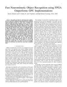
Fig. 1. Multi sensor data sets related to a common manifold. For each rotation angle of the head we are given two images, one from each row. We seek the common manifold, which encodes the head position (rotation angle).

To introduce and motivate our approach, consider the multisensor data set depicted in Fig. 1. The two synchronized image sets correspond to a person rotating his head from left to right. We consider each image as a signal in a highdimensional space (of O(104 )). (In a real application, the image set might contain X-ray and MRI images.) Despite the dissimilar appearance, both sets are the manifestations of the same phenomenon (a rotating head), and the same latent variable. The variation between the images is essentially one dimensional, as the rotation can be parameterized by a single rotation angle. We are not interested in the spatial domain pixelwise variation within a single image, but in the variations between the different images. By reducing the dimensionality of each input channel, we aim to recover a common parametrization corresponding to the rotation angle. Thus, the multi sensor embedding might improve the recognition of configurations related to the head position (rotation angle). The dissimilar appearance also implies that the density of both sets will differ. More particularly, consider a kernel density estimation scheme [3] applied to each set. Since the distances between images in each set will differ, so will the

2

density. Spectral embeddings (parameterizations) are known to depend on the density of the embedded data set [4]. In order to find a common ground in terms of density, the natural choice is to normalize the density of each set, and embed the sets under uniform density. This notion is formalized by the Laplace-Beltrami embedding and presented in Section III-A. In this work we provide two main contributions: In our core contribution, we propose to utilize Diffusion Maps [5], [4] to derive a unified representation of heterogenous data sources, corresponding to the same underlying phenomenon and manifold. Since our data sources are physically different, as with audio and video, they cannot be combined in their original form. However, their low-dimensional embeddings are in a common form that, most importantly, can be composed. We apply these approaches to audio visual speech recognition, and show that the use of heterogeneous data sources improves accuracy when compared to any single data source. The specific importance of density-invariant embeddings [6] and their use in pattern recognition applications is underscored. This is the new application contribution in the paper. Second, based on the proposed fusion scheme, we present a multi-sensor supervised pattern recognition framework for “group objects”. We apply the Hausdorff Distance [7] to learn and recognize “group objects” and derive a diffusion coordinates selection scheme. Namely, given the diffusion coordinates (spectral embedding) of a heterogeneous or homogeneous data source, we suggest an algorithm for choosing a subset of the coordinates that maximizes the Hausdorff classification margin, and improves the recognition rate. The paper is organized as follows: a survey of prior art in multi sensor data analysis is given in Section II. We summarize density invariant embeddings and spectral extensions in Section III, while two complementary approaches for the selection of the kernel bandwidth are presented in Section III-C. Our extension to group recognition is described in Section V and discussed in Section V-D. The new approach to diffusion coordinates selection is given in Section VI. We exemplify and verify our approach experimentally by applying it to audio-visual speech recognition in Section VII. Summary and concluding remarks are given in Section VIII. II. BACKGROUND Multisensor data analysis and fusion is discussed in multiple disciplines such as signal processing, biology, and image processing, to name a few. As a result, many different techniques have been proposed, which can be categorized into addressing two fundamental versions of the problem, the first being to recover an underlying process and the second for taskoriented fusion schemes. As we show, our technique builds upon an approach in the first class but is applicable to both. We stress, however, that only by defining proper classification methodologies can it be made to work at acceptable rates. The first class of problem involves data driven schemes designed to recover an underlying process that is manifested by the multisensor data. Multisensor registration of images is perhaps a paradigm example. In multi-modal medical imaging (MRI, CT), for example, the different image acquisition

processes give rise to individual pixel (voxel) relationships that are complex and difficult to model. Hence, multisensor image alignment is typically based on deriving canonical image representations that are invariant to the dissimilarities between the sensors, yet capture relevant image structure. The underlying structures are geometric primitives, such as feature points, contours and corners [8], [9], [10]. In our technique, of course, we do not have to define these primitives a priori but they should emerge implicitly from the embedding. A more targeted paradigm example is provided by Xia and Kamel [11], who formulate the data fusion problem as the acquisition of multiple input channels that sample the same underlying data source multiplied by different scaling factors. The fused signal is then given by a linear combination of the input sensors, recovered via L1 minimization. In such approaches it is common to model the underlying structure as a random variable or process. Thus, the different sensors are assumed to be different manifestations of the same random variable/process. For instance, in Viola’s work on multisensor image registration [12], multisensor images are modeled as random variables. The motion parameters are estimated by maximizing the mutual information (MI) between the different image modalities, with respect to the motion parameters. The non-parametric probabilities were computed by Parzen windows. Ozertem and Erdogmus [13] used MI to compute pairwise affinities between sensors and thus derive an importance-weighting scheme for each sensor. The scheme is shown to improve the performance of a particle filter based motion tracker. Extending this line, Hidden Markov Models (HMMs) have been widely used to model random processes and statespaces. Pan et al. [14] analyze audio-visual speech data by constructing two separate HMM models, one for each input channel. The HMM models are then unified by maximizing their mutual information. Hence, the assumption is that there exists a latent stochastic process (say, the speech process) that is manifested by both the audio and the visual processes, each modeled by a HMM. Another class of approaches involve dimensionalityreduction-based schemes. These are of particular interest to us, since our approach is in this class. For these approaches, the notion of the statistical model is replaced by the data manifold. Low dimensional manifolds can then be parameterized and unified. A general purpose approach to high-dimensional data embedding and alignment was presented by Ham et al. [15]. Given a set of a priori corresponding points in the different input channels, a constrained formulation of the graph Laplacian embedding is derived. First, they add a term fixing the embedding coordinates of certain samples to predefined values. Both sets are then embedded separately, where certain samples in each set are mapped to the same embedding coordinates. Second, they describe a dual embedding scheme, where the constrained embeddings of both sets are computed simultaneously, and the embeddings of certain anchor points in both datasets are constrained to be identical. Canonical Correlation Analysis (CCA) is a statistical approach that combines linear dimensionality reduction and fusion. Given two input sources x and y, CCA computes linear

3

projections of x and y such that the projections are maximally correlated. Kidron et al. [16] applied CCA to multisensor event detection, thus deriving a common parametrization of the audio and visual signals. The authors show that the CCA is ineffective in analyzing high dimensional data, as the estimation of the corresponding covariance matrix becomes statistically ill-posed. The issue was resolved by applying a sparsity prior, as the common manifold related to audio/visual events was sparse. CCA was applied by Sargin et al. [17] to open-set speaker identification by integrating speech and lip texture features. The authors also propose a method for synchronizing the speech and lip features using CCA. Although our foundation is different, we shall show how CCA can be utilized more effectively. Spectral embedding was applied to multisensor synchronization by Lafon et al. [18]. They showed that unsynchronized high-dimensional data (images) of the same phenomenon (rotating heads) acquired by different sensors, had a common low-dimensional manifold, and that this common manifold could be recovered by the Laplace-Beltrami embedding. (This motivated our opening illustration.) The low dimensional embeddings of the different sensors were then co-registered to synchronize the rotations of the heads. In this paper we assume the sensors to be synchronized a la Lafon, but further utilize sensor fusion to improve recognition. Our classifier design built onto diffusion embeddings thus extends the Lafon paper significantly. Another class of algorithms is based on Multiple Kernel Learning (MKL) and was introduced by Bach et al. [19], [20]. These approaches can be used to derive multisensor SVM classifiers. In contrast, CCA and the proposed scheme provide a unified representation of the multisensor data that can then be used by any data analysis scheme, not necessarily a binary classifier. Similar to our approach, a different kernel is applied to each data source and the fusion of the different sources is achieved by summing the kernel matrices corresponding to each data source. Lanckriet et al.[21] extended the MKL by deriving a SVM classifier using a kernel matrix that was the weighted sum of the kernel P matrices corresponding to the different data sources K = i wi Ki . The weights {wi } were optimized as part of the SDP optimization used to derive the SVM classifier’s parameters. These approaches were applied to biological data [21], [22]. Gene functional classifications were inferred by Pavlidis et al. [22] by applying MKLSVM classifiers to a heterogeneous data set consisting of phylogenetic profiles and DNA microarray expression measurements. Lanckriet et al.[21] analyzed Yeast functionals that were clustered by a weighted MKL-SVM classifier, trained on a heterogeneous set of five types of data sources. A third class of fusion algorithms has been developed for target or event detection. Although related to the previous schemes, now the focus is to optimize the set of parameters that must be estimated to support detection. For example, Dewasurendra et al. [23] applied the DempsterShafer evidence theory to process information from multiple sensor modalities. This Bayesian framework allows to update incoming data, and consider the reliability of the different sensors. A related problem is discussed by Zhu et al. [24].

The data acquired by different sensors is first compressed at each sensor, before being transmitted to a central processor. They derive an application specific compression matrix, which minimizes the estimate error variance of a parameter, related to the measurements by a linear model. A similar problem in target detection is considered by Sibul et al. [25] and Ghartey et al. [26]. Given a set of sensors that acquire signals from a target, the question is how to optimally fuse the information from all of the sensors, aiming to best estimate the target parameters. Our approach, presented in this paper, relates to all classes of algorithms. First, we recover the underlying manifold of each input sensor separately. In particular, we apply the density invariant embedding (Section III-A) that overcomes the fundamental obstacle posed by the sampling density variation over the different sensors. Second, in Section VI, we derive and apply an application-specific feature selection approach to improve recognition accuracy. This combination of embedding coordinates and feature selection should be useful for many of the problems listed above. III. D IFFUSION EMBEDDINGS AND EXTENSIONS The diffusion framework provides two essential computational tools for pattern recognition: (i) density invariant embeddings (Section III-A) and (ii) the extension of a given embedding to a new set of points (Section III-B). The first tool paves the way for a canonical embedding, invariant to the properties of a particular manifestation of a data source; while the second allows the extension of the knowledge from a learning set to a test set. A broader applicative view and mathematical analysis can be found in [6]. Two quantitative approaches for the selection of the kernel bandwidth ε are presented in Section III-C. A. Spectral and Density-Invariant Embeddings n

Given a set Ω = {xi }i=1 , xi ∈ Rd of data points, we start by constructing a weighted symmetric graph in which each data point xi corresponds to a node. In applications where a distance d(·, ·) already exists on the data, it is customary to weight the edge between xi and xj by w(xi , xj ) = exp(−d(xi , xj )2 /ε), where ε > 0 is a scale parameter (kernel bandwidth). We induce a random walk on the data set Ω by computing the row-normalized Markov matrix M w(xi , xj ) M (xi , xj ) = X , w(xi , xj ) xj ∈Ω

The embedding coordinates for the set Ω are given by the right K eigenvectors and eigenvalues of M M φk = λk φk .

(3.1)

n b = {b b consists bi ∈ RK . Ω Denote the embedding Ω xi }i=1 , x K of {φk }k=1 spectral embedding vectors. Each embedding vector φk is of length n, and is the k 0 th spectral coordinate. Thus, the i0 th entry in φk , is the k 0 th spectral coordinate of the sample xi . This is depicted in Fig. 2.

4

↑  ← x1 →  ↑ ↑  ← xˆ1 →   ↑ Spectral       M M n  → Embedding →   =  φ1 L φK  n  ← xˆ →   ↓ ↓  ← xn →  ↓  ↓ n    ← d → ← K → ← K → Fig. 2. Embedding the dataset. Given a set of n samples {xi }n i=1 , xi ∈ Rd we compute K eigenvectors, each of length n. Each eigenvector is a spectral embedding coordinate, and the embedding of each sample is given b i ∈ RK . by {b xi }n i=1 , x

Density-invariant embedding [4], [6] is essential to our application. Its focal point is to make the embedding reflect only the geometry of the data and not its density. Classical eigenmap methods [27], [28], provide an embedding that confounds information about the density of sample points and the manifold geometry, so the embedding coordinates heavily depend on the density of the data points. To remove the influence of the density of the data points, we renormalize the Gaussian edge weights wε (·, ·) with an estimate of the density and then compute the Graph-Laplacian embedding. This is summarized in Algorithm 1. Algorithm 1 Approximation of the Laplace-Beltrami diffusion 1: Start¡ with a rotation-invariant kernel wε (xi , xj ) = ¢ exp −kxi − xj k2 /ε . 2: Let qε (xi ) be an estimate of the density per sample point X qε (xi ) , wε (xi , xj ) (3.2) xj ∈Ω

and form the new kernel w eε (xi , xj ) = 3:

wε (xi , xj ) . qε (xi )qε (xj )

Apply the normalized graph Laplacian construction to this kernel, i.e., set w eε (xi , xj ) M (xi , xj ) = X . w eε (xi , xj ) j

4:

The density invariant embedding is given by the eigenvectors of M M φ l = λl φ l

B. Out of sample extension In most recognition tasks it is essential to extend the lowdimensional representation computed on a training set to n new samples. Let Ω = {xi }i=1 , xi ∈ Rd be a data set, n K b = {b bi ∈ R its spectral embedding, and {φk }K Ω xi }i=1 , x k=1 the corresponding diffusion embedding vectors, either density invariant or not. We present an approach for computing the embedding of a new point, y ∈ Rd , y ∈ / Ω, without having to embed the superset {Ω, y}. The embedding is extended to y K by extrapolating the spectral embedding vectors {φk }k=1 to y, using the Nystr¨om extension method [29]. Following Eq. K 3.1, the spectral embeddings {φk }k=1 are the eigenvectors of

a positive semi-definite (p.s.d.) matrix, and the Nystr¨om extension extrapolates the eigenvectors of p.s.d kernels (matrices) to new points. Thus, by extending the K embedding vectors b ∈ RK that to the point y, we get a K dimensional vector y is the spectral embedding of y. For ease of presentation, we apply the extension scheme to a Gaussian kernel, while other p.s.d kernels can be used mutatis mutandis. Let σ > 0 be a scale of extension, and consider the eigendecomposition of a Gaussian kernel of width σ on the training set Ω: X 2 2 µk φjk = e−kxj −xi k /σ φik , xj ∈ Ω . i

φik

0

where is the i th entry of the vector φk . As the kernel can be evaluated at any point in Rd , it is possible to take any y ∈ Rd in the right-hand side of this identity. This yields the following definition of the Nystr¨om extension of φk from Ω to Rd : 1 X −ky−xi k2 /σ2 i φ∗k , e φk , y ∈ Rd , (3.3) µk i where φ∗k is the extended value of the eigenvector φk at the K point y. By applying Eq. 3.3 to the K eigenvectors {φk }k=1 , b , the embedding of y. we derive y C. Kernel Bandwidth Selection In this section we discuss the selection of the kernel bandwidth parameter ε, used in Section III-A to derive the spectral embedding. For that we provide two data-driven approaches. The first, suggested by Singer et al. [30], and denoted by the Singer measure (SM ), is based on an asymptotic analysis of the discrete Markov walk induced by the spectral embedding on the data set [31]. By analyzing the discretization error of the discrete Markov walk, it is shown [30] that the following functional X X ¡ ¢ SM (ε) = wij = exp −kxi − xj k2 /ε i,j

i,j

can be used to characterize the discretization error. The sweet spot of this curve, in terms of discretization error, is the interval of ε for which the curve is linear in a log-log plot of SM (ε). The second approach, denoted the max-min measure, is based on the notion that spectral embeddings agglomerates local parameterizations of the data manifold to derive a global parametrization. More accurately, ε should be chosen such that the kernel describes the infinitesimal connectivity of the data set. Thus, we choose ε to be as small as possible while maintaining its local connectivity. In practice, we use the following local connectivity measure ¡ ¢ Hi (ε) = min kxi − xj k2 , i 6= j (3.4) j

Thus, Hi (ε) is the minimal distance connecting the data point xi to its neighborhood. The kernel bandwidth is then set as ε = C max (H (ε))

(3.5)

where C is typically in the range of 2-3. We provide experimental validation of both approaches in Section VII-B.

5

IV. M ULTI - SENSOR FUSION With the background in place, we now present the proposed data fusion scheme. For the sake of clarity, we restrict our discussion to the case of two input channels; the extension to an arbitrary number of channels is straightforward and is discussed later in this section. Suppose we are given two sets of measurements, Ω1 , Ω2 related to ª © a singleª phenomenon Ω = {x1 , ...,x © n }, where Ω1 = x11 , ..., x1n , x1i ∈ Rd1 and Ω2 = x21 , ..., x2n , x2i ∈ Rd2 . We seek to fuse Ω1 and Ω2 by computing a unified n b = {b low-dimensional representation Ω zi }i=1 . It is assumed that Ω1 and Ω2 are aligned, implying that x1i and x2i relate to the same epoch of xi . We start by computing the Laplace ©Beltrami Embedding ªn b1 = x b1i i=1 , x b1i ∈ RK1 (LBE) of Ω1 and Ω2 , denoted Ω © 2 ªn b2 = x b2i ∈ RK2 , respectively. Each embedding bi i=1 , x and Ω reflects the geometry of the data as viewed by that sensor. To combine these representations into a unified representation n {b zi }i=1 , we compose them to form µ 1¶ bi x b . (4.6) zi = b2i x b is made of n vectors of dimension K1 + K2 . Ω L Given L input channels {Ωl }l=1 , one would compute n oL bl , the embeddings of the L input channels, and Ω l=1

combine the embedding coordinates  1 bi x  ..  b zi =  .  .

(4.7)

bL x i As before, each input sensor might have a different embedding dimensionality Kl . A. Discussion In this section we relate and compare the proposed fusion scheme to CCA and MI. Experimental comparisons to CCA are presented in Section VII. Given multi sensors data sources (such as audio and video) whose manifestations are dissimilar, these approaches (and ours) implicitly assume that the different sources are related by a common latent representation. The geometrical embedding approaches (CCA and ours) assume that there exists a common low-dimensional manifold. CCA assumes it to be linear and proposes an optimal numerical scheme for its recovery, while our approach allows nonlinear manifolds. In contrast, MI implicitly assumes a common statistical model. These assumptions are application driven and axiomatic. For instance, there are dozens of papers on registering multisensor medical images by MI [12]. Non of them proved that there exists a common probability distribution among the multi modality images. We assume its existence due to their perceptual similarity, overlooking the dissimilar appearance. We also assume, due to the setup of the acquisition process, that the input images capture the same body parts. If these assumptions do not hold the registration will fail. The same applies to CCA, but there the common

latent representation is a linear manifold. If it fails, the CCA will provide inferior results (see Section VII). Another issue to consider is the numerical stability and accuracy. The CCA is based on eigendecomposition that is numerically stable and recovers the common linear manifold optimally. But, it is susceptible to the ‘curse-of-dimensionality’ due to the estimation of the covariance matrix [16]. Our scheme assumes a common nonlinear manifold and is applicable for high-dimensional data. It also handles the sampling density issue. The estimation of MI of high dimensional data sources is ill-posed due to the ‘curse-of-dimensionality’, and even for low-dimensional data, one has to resolve certain implementation details (density estimation scheme, interpolation etc.). V. G ROUP R ECOGNITION IN D IFFUSION S PACES The mathematical foundations laid in the previous sections pave the way for a data classification scheme able to handle group objects. Each group object consists of a set of high dimensional samples. Most state-of-the-art classifiers, such as SVM and NN, classify a single high-dimensional sample at a time, and there is no notion of a group. In the context of this |S| paper, we denote each such group as a signal S = {xi }i=1 . For instance, a signal S might be the utterance of a digit that consists of a set of high dimensional samples (vectors), each sample xi ∈ Rd being a temporal window. Given that there are C different classes of signals, we derive a recognition © ª|T | scheme able to classify an input test signal T = xTi i=1 to a particular class. The analysis of high dimensional signals, such as audio and video signals is of particular interest and utilizes low dimensional embeddings as discussed in the previous sections. In particular, the spectral fusion scheme allows us to represent multiple heterogeneous sources by a unified spectral embedding in RK , extending the application of those techniques for representing the input as a single channel. This implies that we can utilize the same classifier for both single (audio,video) and multi-sensor (audio/visual) data. We now develop this into our group recognition scheme, which consists of three phases: learning the data manifold, learning the training signals, and finally, recognition. Each is considered in turn. A. Learning the data manifold of the input sensors We start by learning the manifold of the high dimensional samples using spectral embedding. The manifold is learnt by n b = {b bi ∈ RK of a set computing the embedding Ω xi }i=1 , x n d of samples Ω = {xi }i=1 , xi ∈ R ; thus it should span the space of the input source. For instance, a set corresponding to the speech manifold of a speaker is acquired by having the subject read aloud an article. We thus assume that the article contains all possible phoneme and mouth positions. b will be later used to efficiently compute The embedding Ω the embeddings of other input samples, via out-of-sampleextension (Section III-B). When the input dataset consists of a single sensor, one can use either the Graph Laplacian Embedding (GLE) or the density invariant LBE. But, when dealing with a multi sensor dataset, one has to use the LBE to fuse the input sensors.

6

B. Learning the training signals In this phase the signals are known to consist of C classes c = 1, 2, ..., C; for our speech recognition example C = 10, corresponds to the digits ‘0’,..,‘9’. We are also given the b sample learning set Ω and its embedding Ω. C We are given C sets of training signals {Ac }c=1 |A |

Ac = {Sic }i=1c ,

(5.8) o|Sic | n where Sic = xc,i is a training signal. This hierarchy is j j=1

depicted in Fig. 3. We start by computing the embedding of the training signals. The embedding of a signal Sci is given by Sbic = o|Sic | n bc,i x , the embedding of its samples. Sbic has the same j j=1

number of samples (vectors) as Sic , each being an embedding n o|Ac | bc = Sbci of dimension K. We denote by A the embedding i=1 of a training set, given by the embeddings of its training signals. n oC The embedding hierarchy is also depicted in Fig. 3. bc b of the A is computed by extending the embedding Ω c=1

C

learning set to each sample x ∈ {Ac }c=1 .   A1 ,..., Ac ,..., AC  { { {  " c −1" "9"   "0"

{

Ac = S1c ,..., Sic ,..., S cAc

{

Sci = x1c ,i ,..., x cS,ci i

}

  Aˆ1 ,..., Aˆc ,..., AˆC  { { {  "0" "c −1" "9"  

}

{

Aˆc = Sˆ1c ,..., Sˆic ,..., Sˆ cAc

spectral embedding

{

Sˆci = xˆ1c ,i ,..., xˆ cS,ci i

}

}

Fig. 3. The data hierarchy of the group recognition problem. Each item to recognize is a signal Sci consisting of high dimensional samples. For recognition purposes, we are given {Ac }C c=1 sets of training signals.

to compute and assumes that both sets are given in the same coordinates system. It naturally handles nonlinear elastic deformations between the sets. As such, it is suitable for the group object recognition problem in general and the audiovisual task in particular. It follows by Eq. 5.9 that the SHD is determined by a single pair of samples a ∈ S1 and b ∈ S2 that are the furthest away, among all pairs of nearest neighbors in S1 and S2 . This observation paves the way for the iterative SHD feature selection scheme presented in Section VI. Given the SHD that quantifies the distance between Tb and the embedding bc , one can train and apply a variety of the training sets A of classification schemes, such as SVM, LDA and K-NN classifiers. In order to exemplify the effectivity of sensor fusion process we applied the 1NN classifier c∗ = arg

min c = 1..C i = 1.. |Ac |

dH (Tb, Sic ),

(5.10)

∗

Simply put, we look for the training signal Sic whose embedding is the closest to Tb, and classify T as T ∈ c∗ . D. Discussion The proposed scheme has several practical advantages. First, b needs to be computed only once the manifold embedding Ω and it can be done offline. Second, the training phase of our C scheme is fast. The embedding of the training sets {Ac }c=1 can be done on the fly. Adding a new class of signals C b Finally, c∈ / C does not require to recompute {Ac }c=1 or Ω. the embedding of each testing point x ∈T or training point C x ∈ {Ac }c=1 is computed independently, and can be fully parallelized for real-time applications. Our approach treats temporal signals, such as speech (audio and visual samples) as sets of points in high dimensional space, overlooking their temporal information. While the temporal information might improve recognition somewhat, we adopted this approach for two key reasons: (i) its ability to handle temporally unsynchronized signals; and (ii) its ability to handle missing samples.

C. Test signal recognition We conclude with the signal recognition step, where given © ª|T | a test signal T = xTi i=1 , xTi ∈ Rd we aim to identify its corresponding class c∗ . For that, we compute Tb the embedding VI. S PECTRAL FEATURES SELECTION of T by way of spectral extension as before. Simply put, Our recognition scheme is based on computing the SHD the spectral extension, allows us to position both the training between sets of points. In this section we derive a feature and test sets within the same K-dimensional diffusion based selection scheme that improves the recognition rate by maxcoordinates system. imizing the SHD classification margin. We emphasize that Given the embeddings of the Learning and Test sets, we other common feature selection approaches [3], [32], such as require a group object similarity measure, able to quantify the d discriminant analysis (LDA, QDA) and SVM are inapplicable notion of distance between sets of points in R . For that we utilize the Symmetric Hausdorff Distance (SHD) [7]. Given to group recognition, since they maximize the recognition two points sets S1 ∈ Rd and S2 ∈ Rd , the SHD dH (S1 , S2 ) margin of a single sample, and not that of a group (signal). Let S c be a signal belonging to the class c, its SHD is given by ½ ¾ margin ∆ (S c ) is given by classification 2 2 dH (S1 , S2 ) = max max min {kx1 − x2 k }, max min {kx1 − x2ck } . x2 ∈S2 x1 ∈S1 x1 ∈S1 x2 ∈S2 min dH (S c , Sic )− min dH (S c , Sic ) ∆ (S ) , min i=1..|Ac | (5.9) c = 1..C i=1..|Ac | The SHD is a min-max distance that does not require the c 6= c matching or alignment of the sets S1 and S2 . It is fast (6.11)

7

∆ (S c ) is the difference in SHD scores between the best false classification of S c (first term on the r.h.s of Eq. 6.11), and the best true classification (second term on the r.h.s of Eq. 6.11). We aim to have ∆ (S c ) À 0 as the signal S c is expected to be closer to the signals in c rather to those in c 6= c. Our supervised approach to feature selection utilizes two given training sets of signals AcF ∈ / c and AcT ∈ c. We aim to compute a vector of class specific weights wc ∈ RK , K X c wm = 1, such that it maximizes the weighted SHD margin m=1

∆w (S c ) , min dH (WC S c , WC S)− min dH (WC S c , WC S), S∈AF

S∈AT

(6.12) where WC is a K × K diagonal matrix with wc as its main diagonal. By WC S we imply that each sample x ∈S, x ∈ RK is pointwise weighted by wc . The optimal weight vector wc is given by c

c

wc (S ) = arg max ∆w (S ) . w

(6.13)

For now, we show how to maximize the margin for a particular training sample S c ; we will later generalize the scheme for a set of training samples {Sic }. Solving Eq. 6.13 directly can prove difficult, since for each weight vector wc there could be different nearest neighbors within the computation of the SHD. Hence, we propose the following iterative scheme. We start by assuming a uniform 1 c weight vector wc , wm = K ∀m. Given wc , Eq. 6.13 can be simplified by searching over AcT and AcF for the signals closest to S c SF = arg minc dH (WC S c , WC S)

we choose the P features with the largest margins ∆ (S c ). Finally, to gain robustness, we compute the average margin per feature ∆c , by averaging the margins ∆m (S c ) of all of the signals in AcT 1 X ∆ (S c ) . ∆c = c |AT | c c S ∈AT

As before, we choose the P features with the largest margins. Given the updated weight vector wc , we reiterate the process. This procedure is repeated for all C classes, each having its own weight vector wc . We found this scheme to converge within 2-3 iterations and provide improved recognition rates for small numbers of features. More experimental details are provided in Section VII. VII. E XPERIMENTAL RESULTS Our sensor fusion scheme was put to the test by applying it to audio-visual speech recognition. We compare the proposed multi sensor analysis scheme to visual-only and audioonly recognition and show an accuracy improvement. This application was chosen as it is a classical example of multisensor based recognition. In Section VII-E we compare our fusion scheme to PCA and CCA, because these are considered state-of-the-art techniques [16], [17]. That our performance compares demonstrates the power of the embedding coordinates; that they can be used to extend the above techniques demonstrates their potential power. A. Data acquisition and preprocessing

We recorded several grayscale movies depicting the lips of a subject reading a text in English together with the audio and track. The recording was made with a regular DV camera and ST = arg minc dH (WC S c , WC S). the audio was sampled at 32KHz. S∈AT Each video frame was automatically cropped into a rectan¡ Fa ¢ c Fa We can then find the pairs of samples, a ∈ S , b ∈ S F gle of size 140 × 110 around the lips, and was considered as a ¡ ¢ and aT r ∈ S c , bT r ∈ ST that determine the SHD margin. point in R140×110 . The frames were normalized to have zero Inserting those into Eq. 6.12 we get mean and unit variance. K K X X ¡ Fa ¢ ¡ Tr ¢2The audio signal was broken up into overlapping timec c 2 Fa 2 c 2 T rwindows centered at the beginning of each video frame. Since ∆w (S ) = (wm ) am − bm − (wm ) am − bm the video is sampled at 25 frames per second, we formed audio m=1 m=1 (6.14) windows 80ms long (equal in duration to two video frames) K ³¡ and reduced the frame-splitting artifacts by smoothing with a X ¢ ¡ Tr ¢ ´ c 2 a Fa 2 Tr 2 = (wm ) aF − b − a − b bell-shaped function. We computed the log of the magnitude m m m m m=1 of the FFT of each window, retaining only half of it, due to K X the conjugate symmetry of the FFT. We then computed the c 2 = (wm ) ∆m (S c ) , discrete cosine transform (DCT) of the result. This produces m=1 a feature vector in R1280 . To reduce the volume of the dataset c where ∆ (S ) is the margin per feature. we averaged the vector into 256 uniform bins. K X Using the conventions of Section IV, the set ΩA ∈ R256 c Given that wm = 1, one is tempted to adopt a greedy corresponds to the audio samples, while Ω ∈ R15400 correV m=1 approach to maximize the margin ∆ (S c ) in Eq. 6.14 such that sponds to the set of video frames. Note that in this setup ΩA c a single element is set to wm = 1 and the rest are set to zero, and ΩV are naturally aligned and contain the same number of 0 points. where c Following Section V, the manifold learning dataset conm0 = arg max ∆m (S ) . m sisted of 6000 video frames (and as many audio windows), In practice this approach proved to be too greedy, so we only corresponding to the speaker reading a press article. We will used ∆ (S c ) as a ranking measure. Then, at each iteration, refer to this data as text data. In order to acquire the training S∈AF

8

The audio and visual text data sets were embedded using the LBE discussed in Section III-A. In order to set the kernel bandwidth ε, we applied both the approaches presented in Section III-C. Figure 4 depicts both bandwidth selection measures for the audio and visual data sets. Based on Figs. 4a and 4c, and using a multiplier of C = 2 in Eq. 3.5, we set εA = 200 for the audio data and εV = 5000 for the video data. Examining the other measure in Figs. 4b and 4d, it is evident that these values coincide with the linear interval of the curve. Audio

94

94

92

92

90 88 86

88 86 84

84

82

82 80 100

90

80 150

200 ε

250

300

0.5

(a)

1

1.5 ε

(b)

2

2.5

3 4

x 10

Fig. 5. The recognition accuracy using a single sensor vs. the kernel bandwidth ε. The green dot marks the ε value based on the ‘max-min’ criterion. Varying ε over a wide range does not change the recognition accuracy significantly.

Audio

90

Video

Audio

Accuracy [%]

B. Data fusion and Kernel bandwidth selection

bandwidth. For these tests we used LR = 0.5, LBE and Nev = b A ∈ R20 and 20 diffusion coordinates per channel, such that Ω 20 b ΩV ∈ R . The Nev spectral features were chosen according to their eigenvalues’ magnitude. (The first eigenvector taken is the one corresponding to the largest eigenvalue.)

Accuracy [%]

and test sets of digits, we asked the subject to repeat each digit “zero”, “one”, ... , “nine” 50 times. We will refer to this data as digits data. A typical digit consists of 20-30 samples.

80 7

10

70

60 6

10

50

40

5

30

10

20

C. Density invariant embedding

10 4

10

0

0

1000

2000

3000

(a)

4000

5000

1

2

10

6000

i

3

10

(b)

10

ε

In this section we study the use of density invariant spectral embeddings for the single and multi sensor cases. We start by computing the approximate densities of ΩA and ΩV . Recalling that the density is positive and depends on the dynamic range of the data set, we use the following measure for evaluating the density uniformity

Video

Video 2500

7

10

2000

6

1500

10

1000 5

10

500

U (Ω) =

4

10

0

0

1000

2000

3000

(c)

i

4000

5000

6000

2

10

3

10

(d)

4

ε

10

Fig. 4. Setting the kernel bandwidth ε. The maximal minimal distance per sample is shown in (a) and (c), for the audio and visual data, respectively. It is common to set ε to be twice as large as the maximal minimal distance. In (b) and(d) we compute the measure suggested by Singer [30]. The interval of ε for which the measure is linear is the preferred one.

All of the spectral embeddings were computed using the Gaussian kernel exp(−kxi −xj k2 /ε), and the test and training sets were created by randomly splitting the digits data into two parts. We denote the ratio of the learning set to the digits data the learning ratio LR. Following the second step in Section V we extended the spectral embeddings from the text data to the digits data. These embeddings were computed separately for b A and Ω b V , respectively. The unified ΩA and ΩV , and denoted Ω b AV . Denote the corresponding embedding is then given by Ω Hausdorff distance based classifiers HA , HV and HAV for the audio, visual and unified classifiers, respectively. We b A and Ω b V were used emphasize that the same embeddings Ω to derive all classifiers. We then applied HA and HV to study the sensitivity of the recognition rate to the choice of the bandwidth ε. The results are reported in Fig. 5, where we measured the recognition rate of each channel separately. The recognition rate is averaged over all ten digits. The recognition is robust to changes of the

std (D (Ω)) mean (D (Ω))

(7.15)

where D is the density of each dataset. The density was computed by kernel based density estimation, using Gaussian kernels with the bandwidth computed in the previous section. The same one was used for the spectral embedding. The density comes out to be UV (Ω) = 0.0456 and UA (Ω) = 0.2531. It follows that the density of the visual channel is more uniform than that of the audio one. In terms of manifold learning, this implies that the visual signal was able to uniformly span the space of speech states. Figure 6 studies the influence of the density invariant embedding on the classification accuracy. We report the classification results for both the single and multi sensor cases, where the data is embedded using both the LBE and GLE. By that we aim to experimentally verify the conjecture used throughout this work: the notion that the audio and visual data are different manifestations of a common underlying lowdimensional process. Using the LBE, both ΩA and ΩV are represented in their common diffusion coordinates system. Figures 6a-6b compare the classification results in the single channel case (ΩA and ΩV ) using the LBE and GLE, using LR = 0.5 and Nev = 20. There is no significant difference in the recognition accuracy of the LBE and GLE. In contrast, Fig. 6c depicts the classification results for our proposed sensor fusion scheme, where the LBE outperforms the GLE.

9

Visual

90

90

85

85

80 75 70 65 5

10 #Eigenvectors

15

75 70 65

Laplace Beltrami Graph Laplacian

60 0

80

Laplace Beltrami Graph Laplacian

60 0

20

5

10 #Eigenvectors

(a)

15

We then studied the feature selection scheme introduced in Section VI, where we use the same number of coordinates Nev for all classifiers. The results are shown in Fig. 8, where the feature selection performed well for all classifiers, being superior to the common approach of selecting the spectral coordinates according to their eigenvalues.

20

Unified

(b)

Unified Accuracy

95

Accuracy [%]

90 85

Audio

95

95

90

90

85

85

80

80

Accuracy

95

Accuracy [%]

Accuracy [%]

Audio 95

75 70 65

80

60

75

55

70

50 0

65 5

10 #Eigenvectors

15

70 65 60

Beltrami with feature selection Beltrami

5

10 Features#

15

Beltrami Beltrami with feature selection

55 50 0

20

5

10 Features#

(a)

Laplace Beltrami Graph Laplacian

60 0

75

15

20

(b)

20

Visual 95

(c)

90

Accuracy

85

Fig. 6. Digits recognition results for Laplace Beltrmi (density invariant) and Graph Laplacian embeddings. (a) and (b) depict the recognition accuracy of the single sensor classifiers. (c) The recognition results of the unified sensor scheme.

80 75 70 65 60 Beltrami Beltrami with feature selection

55 50 0

Given the classifiers HA , HV and HAV , we compare their recognition accuracies in Fig. 7. In the multi sensor case, we use Nev embedding vectors from each input channels (2Nev embedding vectors overall). For small number of coordinates, Nev ≤ 8, the unified classifier performs as well as the HV , which is the best of HA and HV . But, for Nev > 8 we begin to witness the fusion effect, as the proposed fused classifier HAV is able to outperform each of the single sensor classifiers HA and HV . In particular, the recognition rate of HV , the best of the single sensor classifiers saturates around 88%, while the unified one HAV , achieves an accuracy of up to 95%. Adding more diffusion coordinates (Nev > 20) to HA and HV did not improve the classification accuracy.

15

20

Fig. 8. Feature selection results. The feature selection scheme outperforms the naive selection approach for all classifiers.

As for computational complexity, the proposed scheme is asymmetric by nature. Namely, most computations are done offline, computing the manifold embedding vectors, so that the recognition step is fast. The typical running time for the preprocessing of 6000 audio and visual frames, and the computation of the spectral embeddings was approximately 3 minutes. We run our Matlab implementation on an Intel(R) Core(TM)2 Duo running at 2.20GHz with 4GB of memory. The recognition of a single digit, consisting of 40 samples on average, took an average of 0.5 seconds. E. Comparison to Canonical Correlation Analysis and Principal Component Analysis

95 90 85 Accuracy [%]

10 Features#

(c)

D. Unified recognition results and feature selection

80 75 70 65 60

Unified Audio Visual

55 50 0

5

5

10 #Eigenvectors

15

20

Fig. 7. Digits recognition vs. the number of embedding coordinates for audio, visual and audio-visual data. All channels were embedded using a density invariant embedding. The unified audio-visual scheme significantly outperforms the single sensor recognition.

We compared the proposed unified recognition approach to linear dimensionality reduction schemes based on Principal Component Analysis (PCA). Those were found to be useful in previous works [16], [17]. The results are depicted in Fig. 9 and the maximal recognition rates for each scheme are reported in Table I. First, we applied CCA directly to the audio/video features. The recognition rate was quite low, topping at 66.7%, compared to the 94.8% achieved by the proposed scheme. The CCA aims to recover the two most correlated linear components, one from each sensor. Yet, in high-dimensional signals, such as our audio/video data, this assumption might prove too restrictive, as the signals are related by non-linear transforms. We also applied PCA to both sensors separately and appended the embeddings, the same way we fused the spectral embeddings in Section IV. The resulting recognition rate was up to 91.75%. Motivated by that,

10

Accuracy [%]

we applied the CCA and PCA to the spectral embeddings. The CCA improved the recognition rate significantly, and achieved the a recognition rate of 96.5%, the highest over all schemes. Applying the PCA to the spectral embeddings gained an accuracy of 95.1%. This is attributed to two fundamental issues: first, the CCA recovers the most correlated linear structures within the data, while the Diffusion Framework recovers non-linear structures. Second, Kidron et al. [16] show that the CCA is ineffective in analyzing high dimensional data, as the estimation the corresponding covariance matrix becomes statistically ill-posed. In [16] the issue was resolved by applying a sparsity prior, as the common manifold related to audio/visual events was sparse along the temporal axis. This is not the case in our data. To conclude, the proposed spectral embedding was able to provide better recognition rate then the PCA. Moreover, judging by the performance of CCA applied to the original dataset, it follows that the audio and video signals do not have a common linear manifold. Yet, when applied to the spectral embedding the CCA provided the best result overall. This reinforces the notion that the spectral embedding was able to extract a common nonlinear manifold.

95 90 85 80 75 70 65 60 55 50 45 40 35 30 0

Diffusion Unified CCA Unified CCA Diffusion Unified PCA Diffusion Unified PCA Unified

5

10 #Eigenvectors

15

20

Fig. 9. Recognition rates for the different sensor fusion schemes. The maximal retrieval rates are reported in Table I.

Rate

Spectral 94.82%

Spectral+PCA 95.1%

Spectral+CCA 96.52%

CCA 66.79%

PCA 91.75%

TABLE I R ETRIEVAL RATES FOR THE DIFFERENT SCHEMES .

VIII. S UMMARY AND C ONCLUSIONS In this work we introduced and tested a multisensor data analysis scheme, based on spectral embedding. The scheme was applied to audio-visual speech recognition. We embedded each data source separately and then appended the embeddings to derive the fused representation. The success of the scheme

provides some evidence that data manifolds can be “composed” in support of recognition. Such compositions could emerge as a fundamental tool in the future. Our recognition approach was explicitly based on the notion of group recognition, and an original contribution of this work was the development of a corresponding novel feature selection scheme. This provides a data point to confirm the power of diffusion coordinates as a foundation for recognition algorithms and extends the basis for classifiers to work with them. Diffusion embeddings require the specification of a resolution or bandwidth parameter in the kernel, and we also detailed two data-driven approaches for the selection of it. In summary, the experimental results show that the fusion effect is indeed achieved, and that multisensor based recognition can be made superior to single-sensor classifiers. Our final result, that PCA analysis applied to the spectral embedding further improves the recognition rate, suggests that even more is possible. Perhaps this is because even linear techniques can yield improvements when the requisite non-linear structure is captured by proper embeddings. R EFERENCES [1] J. Driver, “Enhancement of selective listening by illusory mislocation of speech sounds due to lip-reading,” Nature, no. 381, pp. 66–68, 1996. [2] Y. Gutfreund, W. Zheng, and E. I. Knudsen, “Gated visual input to the central auditory system,” Science, no. 297, pp. 1556–1559, 2002. [3] T. Hastie, R. Ribshirani, and J. Friedman, The elements of statistical learning: data mining, inference and prediction. Springer, 2002. [4] R. Coifman, S. Lafon, A. Lee, M. Maggioni, B. Nadler, F. Warner, and S. W. Zucker, “Geometric diffusions as a tool for harmonic analysis and structure definition of data: Diffusion maps,” Proceedings of the National Academy of Sciences, vol. 102, no. 21, pp. 7426–7431, May 2005. [5] R. Coifman, S. Lafon, A. Lee, M. Maggioni, B. Nadler, F. Warner, and S. Zucker, “Geometric diffusions as a tool for harmonics analysis and structure definition of data: Multiscale methods,” Proceedings of the National Academy of Sciences, vol. 102, no. 21, pp. 7432–7437, May 2005. [6] R. Coifman and S. Lafon, “Diffusion maps,” Applied and Computational Harmonic Analysis: Special issue on Diffusion Maps and Wavelets, vol. 22, pp. 5–30, July 2006. [7] “Hausdorff distance.” [Online]. Available: http://en.wikipedia.org/wiki/ Hausdorff distance/ [8] A. Gueziec, X. Pennec, and N. Ayache, “Medical image registration using geometric hashing,” IEEE Computational Science & Engineering, special issue on Geometric Hashing, vol. 4, no. 4, pp. 29–41, OctoberDecember 1997. [9] H. Li, B. S. Manjunath, and S. K. Mitra, “A contour-based approach to multisensor image registration,” IEEE Transactions on Image Processing, vol. 4, no. 3, pp. 320–334, March 1995. [10] R. Sharma and M. Pavel, “Registration of video sequences from multiple sensors,” in Proceedings of the Image Registration Workshop. NASA GSFC, 1997, pp. 361–366. [11] Y. Xia and M. Kamel, “Cooperative learning algorithms for data fusion using novel l1 estimation,” Signal Processing, IEEE Transactions on, vol. 56, no. 3, pp. 1083–1095, March 2008. [12] P. Viola and I. Wells, W.M., “Alignment by maximization of mutual information,” Computer Vision, 1995. Proceedings., Fifth International Conference on, pp. 16–23, Jun 1995. [13] U. Ozertem and D. Erdogmus, “Information regularized sensor fusion: Application to localization with distributed motion sensors,” J. VLSI Signal Process. Syst., vol. 49, no. 2, pp. 291–299, 2007. [14] H. Pan, S. Levinson, T. Huang, and Z.-P. Liang, “A fused hidden markov model with application to bimodal speech processing,” Signal Processing, IEEE Transactions on, vol. 52, no. 3, pp. 573–581, March 2004. [15] J. Ham, D. Lee, and L. Saul, “Semisupervised alignment of manifolds,” in Proceedings of the Tenth International Workshop on Artificial Intelligence and Statistics, Jan 6-8, 2005, Savannah Hotel, Barbados, pp. 120–127.

11

[16] E. Kidron, Y. Schechner, and M. Elad, “Cross-modal localization via sparsity,” Signal Processing, IEEE Transactions on, vol. 55, no. 4, pp. 1390–1404, April 2007. [17] M. E. Sargin, Y. Yemez, E. Erzin, and A. M. Tekalp, “Audiovisual synchronization and fusion using canonical correlation analysis.” IEEE Transactions on Multimedia, vol. 9, no. 7, pp. 1396–1403, 2007. [18] S. Lafon, Y. Keller, and R. R. Coifman, “Data fusion and multi-cue data matching by diffusion maps,” IEEE Transactions on Pattern Analysis and Machine Intelligence, vol. 28, no. 11, pp. 1784–1797, 2006. [19] F. R. Bach, G. R. G. Lanckriet, and M. I. Jordan, “Multiple kernel learning, conic duality, and the smo algorithm,” in ICML ’04: Proceedings of the twenty-first international conference on Machine learning. New York, NY, USA: ACM, 2004, p. 6. [20] F. Bach, “Exploring large feature spaces with hierarchical multiple kernel learning,” in NIPS, 2008, pp. 105–112. [21] G. R. Lanckriet, M. Deng, N. Cristianini, M. I. Jordan, and W. S. Noble, “Kernel-based data fusion and its application to protein function prediction in yeast,” in Proceedings of the Pacific Symposium on Biocomputing, January 2004, pp. 300–311. [22] P. Pavlidis, J. Weston, J. Cai, and W. N. Grundy, “Gene functional classification from heterogeneous data,” in Proceedings of the Fifth Annual International Conference on Computational Molecular Biology, NY, USA, 2001, pp. 242–248. [23] D. Dewasurendra, P. Bauer, and K. Premaratne, “Evidence filtering,” Signal Processing, IEEE Transactions on, vol. 55, no. 12, pp. 5796– 5805, Dec. 2007. [24] Y. Zhu, E. Song, J. Zhou, and Z. You, “Optimal dimensionality reduction of sensor data in multisensor estimation fusion,” Signal Processing, IEEE Transactions on, vol. 53, no. 5, pp. 1631–1639, May 2005. [25] L. Sibul, M. Roan, S. Schwartz, and C. Coviello, “Lossless information fusion for active ranging and detection systems,” Signal Processing, IEEE Transactions on, vol. 54, no. 10, pp. 3980–3990, Oct. 2006. [26] K. Ghartey, A. Papandreou-Suppappola, and D. Cochran, “Time-varying techniques for multisensor signal detection,” Signal Processing, IEEE Transactions on, vol. 54, no. 9, pp. 3353–3362, Sept. 2006. [27] M. Belkin and P. Niyogi, “Laplacian eigenmaps for dimensionality reduction and data representation,” Neural Computation, vol. 6, no. 15, pp. 1373–1396, June 2003. [28] M. Balasubramanian, E. L. Schwartz, J. B. Tenenbaum, V. de Silva, and J. C. Langford, “The Isomap algorithm and topological stability,” Science, vol. 295, no. 5552, p. 7, 2002. [29] C. Fowlkes, S. Belongie, F. Chung, and J. Malik, “Spectral grouping using the nystr¨om method.” IEEE Transactions on Pattern Analysis and Machine Intelligence, vol. 26, no. 2, pp. 214–225, 2004. [30] R. R. Coifman, Y. Shkolnisky, F. J. Sigworth, and A. Singer, “Graph laplacian tomography from unknown random projections,” IEEE Trans. Image Processing, vol. 10, no. 17, pp. 1891–1899, October 2008. [31] A. Singer, “From graph to manifold laplacian: the convergence rate,” Applied and Computational Harmonic Analysis, vol. 1, no. 21, pp. 135– 144, 2006. [32] I. Guyon and A. Elisseeff, “An introduction to variable and feature selection,” Journal of Machine Learning Research, vol. 3, pp. 1157– 1182, 2003.