Auditory Based Feature Vectors for Speech ...

Auditory Based Feature Vectors for Speech Recognition Systems WALEED H. ABDULLA Electrical & Electronic Engineering Department The University of Auckland 20 Symonds Street, Auckland NEW ZEALAND [mailto: [email protected]] Abstract: - Signal processing front end for extracting the feature set is an important stage in any speech recognition system. The optimum feature set is still not yet decided though the vast efforts of researchers. There are many types of features, which are derived differently and have good impact on the recognition rate. This paper presents one more successful technique to extract the feature set from a speech signal, which can be used in speech recognition systems. Our technique based on the human auditory system characteristics. It relies on the Gammatone filterbank to emulate the cochlea frequency resolution. Compared to the standard mel frequency cepstral coefficients and the perceptual linear prediction analysis front ends, our auditory based front-end yielded higher recognition rate when embedded in a continuous hidden Markov model based automatic speech recognition (ASR) system. Also our feature set has better classification characteristics when considering the F-ratio as a figure of merit. Key-Words: - Speech Recognition, Auditory Modelling, Feature Extraction.

1. Introduction A major problem in speech recognition system is the decision of the suitable feature set which can faithfully describe in an abstract way the original highly redundant speech signal. Several techniques have been developed so far for solving this problem. It has been known that the cochlea, the main component of the inner ear, performs the filterbank based frequency analysis on the speech signal to extract the relevant features. Thus, most techniques are pivoting around the filterbank methodology in extracting the features. The difference in the design of the filterbank offers the extraction of different features from the signal. The main parameters in the filterbank filter design are the frequency response, which defines the shape of the filters, the centre frequency and the bandwidth. These parameters can be selected based on the human auditory system. Dominant speech analysis techniques for ASR, namely Mel frequency cepstrum [1] and perceptual linear predictive (PLP) [2], try to emulate the human auditory perception. The Mel cepstrum technique uses filters with centre frequencies spaced equally on a linear scale from 100 to 1000Hz and equally on logarithmic scale above that. Above 1000Hz each centre frequency is 1.1 times the centre frequency of the previous filter. The shape of the magnitude

frequency response of each filter is normally considered triangular. The Q factor, the ratio of the centre frequency to the filter bandwidth, is constant along the whole spectral band. Each vector of log energy calculated from the filterbank outputs is processed by an inverse cosine transform to create what is called Mel frequency cepstral coefficients (MFCCs). The cosine basis attempt to approximate Karhunen-Loeve basis, which provides the necessary decorrelation between the feature vectors, and project the spectrum on directions of maximum global variability [3]. These MFCCs are considered as the extracted features from the speech signal, which in turn are presented to the speech recogniser for classification task. To improve the speech recognition rate the feature vectors are normally augmented by vectors representing the delta (speed) and the delta-delta (acceleration) of the spectral components, MFCCs [4]. The PLP differs from the Mel cepstrum in the type of filter shapes and smoothing of the shortterm spectrum coming out of its filterbank. The Mel cepstrum technique uses the truncation of the MFCCs for smoothing while the PLP approximates the cubic-root compressed modified spectrum by an autoregressive model and computes the model’s cepstral coefficients.

In this paper we develop a compromise between different front ends to design a model that is more coherent than the auditory models, and having the advantages of the Mel cepstrum and the PLP front ends in being fast. Our technique is based on the Gammatone auditory filter bank in extracting the relevant features. Gammatone filter modelling is a physiologically based strategy followed in mimicking the structure of the peripheral auditory processing stage. It models the cochlea by a bank of overlapping bandpass filters. The performance of this technique will be measured using the F-ratio as a figure of merit to show the classification ability of our technique against the classical Melcepstrum and the PLP techniques. Also the recognition rate of a CHMM based ASR system will be compared by using the above three techniques. Our Gammatone based method outperformed the classical Mel-cepstrum and the PLP methods in both classification and recognition rate tests.

2. Gammatone Auditory Filterbank Gammatone filter (GTF) modelling is a physiologically motivated strategy followed in mimicking the structure of the peripheral auditory processing stage. It models the cochlea by a bank of overlapping bandpass filters. The impulse response of each filter follows the Gammatone function shape. This function was introduced by Aertsen and Johannesma [5]. It has the following classical form:

h (t ) = γ ( n , b )t n −1e − bt cos(ωt + φ )u (t )

(1)

Here γ(n,b) is a normalization constant depending on the order, n, and the bandwidth related factor, b, w is the radian centre frequency, φ is the phase shift and u(t) is a unit step function. This function has also been modified for the sake of computation simplification by removing the cosine term from the classical form [6; 7]. The name of this filter derived from its relation to the Gamma function, which has for n>0 the form: ∞

Γ(n ) =

∫t

n −1

e − t dt

(2)

0

The tone is referring to the cosine term, which represents a tone at the centre frequency. Gammatone filter is very similar to the rounded exponential function, reox(p). Reox function is normally used in representing the magnitude response of the human auditory filters [8]. This

function is a parameterisation form of the auditory filters response using notched noise masker technique. It is known that 3rd – 5th order Gammatone filter gives very good approximation to the reox(p) filter over a 60dB range [9]. The main advantage of Gammatone filter over the reox filter is that the former belongs to a linear time invariant system family, while the later does not. This means that the Gammatone filters can be represented by a transfer function and consequently be electronically implemented, while the reox filter lack this property due to unknown phase response [10]. Also, the Gammatone filterbank can very well model the non-linear frequency characteristics of the cochlea even it is belonging to the linear system family. The Gammatone function corresponding to a cochlea filter centered at 1000Hz and with bandwidth of 125Hz is shown in Fig. 1. This figure shows also that the Gammatone function is a good fit to the impulse response of the auditory nerve fibre as measured with reversed-correlation (revcor) technique [11].

Figure 1: The Gammatone function

3. Bandwidth and centre frequency of the GTF The bandwidth of each filter in the Gammatone filterbank is determined according to the auditory critical band (CB) corresponding to its centre frequency. The CB is the bandwidth of the human auditory filter at different characteristic frequencies along the cochlea path. The first determination of the CB was done by Fletcher in 1938 [12]. He assumed that the auditory filters were rectangular, which greatly simplified the formulation of the signal and the noise powers within the CB. Although the rectangular critical band concept is not realistic, it is very useful. The bandwidth of the actual auditory filters can be related to it, by suggesting an equivalent rectangular bandwidth (ERB) filter that has a unit height and a bandwidth ERB. It passes the same power as the real filter do when subjected to white noise input.

This definition of ERB implies the mathematical formula: ∞

∫

2

(3)

H ( f ) df

0

4. Gammatone Filter Implementation

Where the maximum value of the filter transfer function, |H(f)| , is unity. Several physiologically motivated formulas have been derived for the ERB values and our preference is with that suggested by Glasberg et al. [9; 13]. It follows the following formula at centre frequency Fc:

ERB = 24.7(1 + 4.37 f c )

(4)

This formula gives the highest selectivity factor, Q factor, among all the other suggested ones. The Q factor is the ratio between the centre frequency and the bandwidth of each filter. Thus to determine the bandwidth of each filter, which is now represented by the ERB value, the centre frequency of each filter has to be ready beforehand. In the human auditory system, there are around 3000 inner hair cells along the 35mm spiral path cochlea. Each hair cell could resonate to a certain frequency within a suitable critical bandwidth. This means that there are approximately 3000 bandpass filters in the human auditory system. This resolution of filters can not be implemented practically using computational modelling techniques. However we can approximate this high resolution into some possibly implemented one. This can be achieved by specifying certain overlapping between the contiguous filters. The percentage-overlapping factor, v, will specify the number of channels, filters, required to cover the useful frequency band. This band is decided according to the requirements of the application. In our speech recognition system this band is in the range of 100 - 11025Hz, as this is the useful information distribution band. If we depend on Glassberg and Moore [13] recommendation and if we suppose that the information carrying band is bounded by fH Hz and fL Hz with v overlapping spacing the number of filters will be:

N=

9.26 f H + 228.7 ln v f L + 228.7

(5)

Then the centre frequency can be calculated by f c = −228.7 + ( f H + 228.7)e

where

1≤ n ≤ N

−

vn 9.26

(6)

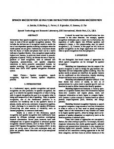
The previous sections described a physiologically motivated way for deciding the bandwidth and the center frequency of each filter in the Gammatone filterbank. The implantation of a bandpass filter from its time domain function is a straightforward procedure in signal processing. It is simply started by finding the Laplace transform of the Gammatone function, then mapping it into the digital form using bilinear transform or impulse invariant transform. There are several methods for representing and implementing the Gammatone function. Lyon suggested an all-pole version, by discarding the zeros from the transfer function of the Gammatone filter aiming for simple parameterization [10]. Lyon’s all-pole version reduces the computation, but at the cost of losing selectivity sharpness at low frequency. Another form was also suggested by Cooke, [7], in which he used the complex data to realize a fourth-order filter. The computations still as that of the eighthorder filter with real data. Cook’s method needs pre-multiplication of the input signal by a complex exponential at the specified centre frequency, filtering with a base-band Gammatone filter, postmultiplication by that exponential. Malcolm Slaney describes one simple way of implementation procedure of the Gammatone based filters [14]. Fourth-order Gammatone filter is also used in the design, as it gives the best reox function fit. It requires eighth-order digital filter to realize. Our preference is with Slaney method, because it preserves the original form of the Gammatone filter and of the simplicity of implementation. The frequency response of a 20-channel filterbank, covering 100-11025 Hz band, after the preemphasis by the equal loudness curve, is shown in Fig. 2. Amplitude Frequency Response

ERB =

Having decided the locations of the centre frequency of each filter the bandwidth can be calculated from (4) and we can now proceed to the implementation stage.

Frequency (Hz)

Figure 2: Frequency … response (6) of a Gammatone filterbank

The bandwidth of the channels is logarithmically proportional with the centre frequency. Fig. 3 shows the relation between the channel number, the centre frequency and the bandwidth. The tips of the filters moving along the centre of the horny shaped curve. The higher the channel number, the lower the centre frequency and bandwidth are, which is consistent with equation (6). The bandwidths of the filters are logarithmically varied with the channel numbers.

feature selection in speaker recognition applications [15]. It is defined as the ratio of the between-class variance (B) and the within-class variance (W). S peec h Signal

Speec h Signal

Ga m ma ton e Filterbank

Ga m ma ton e Filterbank

E qua l Loud ness P re-empha sis

Equa l Loud ness Pre-empha sis

Intensi ty - Loudness P ow er Law

LO G{ }

Invers e D isc rete Fourier Transform

Invers e Disc rete Cosine Transform

Gammatone Filterbank Characteristics

Frequency (Hz)

(a)

A uto Regre ssi ve Mod elling

Smo othin g

Ga m ma-PLP C oeffic ients Channel Number

Figure 3: Gammatone filterbank characteristics

5. Speech analysis using Gammatone filterbank The physiologically motivated Gammatone filters can be used as weighting coefficients for speech signals. In this case the energy within each filter is calculated by finding the magnitude of the Fourier transform of the speech signal and multiplying it by its corresponding weighting filter. The filters’ outputs are subjected to equal loudness preemphasis filter. From this stage we experimented with two options. The first option, Gamma-cepst is warping the energy spectra into cepstral coefficients domain using the inverse cosine transform. This transformation produces highly uncorrelated features, which are necessary for the HMM processing. To reduce the high dimensionality of the analyzed speech into low dimensionality space, a smoothing by truncating the output coefficients to 13 coefficients is necessary. The second option, Gamma-PLP, is to augment similar steps used in preparing the PLP coefficients. The block diagrams of both options are depicted in Fig. 4.

6. Evaluation based on the F-ratio The F-ration is a measure that can be used to evaluate the effectiveness of a particular feature. It has been widely used as a figure of merit for

(b)

Ga m ma-Cep st Co efficients

Figure 4: Block diagrams of two feature extraction paradigms. (a) Gamma-PLP (b) Gamma-cepst

In the contest of feature selection for pattern classification, the F-ratio can be considered as a strong catalyst to select the features that maximise the separation between different classes and minimise the scatter within these classes. The Fratio technique can be formulated as follows: Let us consider that the number of training feature vectors, training patterns, in the jth class of K classes be equal to Nj. Thus the F-ratio of the ith feature can be defined by

Fi =

Bi Wi

(7)

where Bi is the between-class variance and Wi is the pooled within-class variance of the ith feature. These can be mathematically defined by

Bi =

Wi =

1 K 1 K

K

∑ (µ

ij

− µi ) 2

(8)

j =1

K

∑W

ij

(9)

j =1

where µij and Wij are the mean and variance of the ith feature, respectively, for the jth class, and µi is the overall mean of the ith feature. In our approach in using the F-ratio we make use

of the HMM properties to facilitate the implementation of this technique. The HMM technique used is implicitly considering the Gaussian behaviour of the feature vectors which satisfies one condition needed by the F-ratio method. The second condition, uncorrelation, is satisfied by using the diagonal covariance within the structure of the HMM. In our approach we applied the F-ratio, formula (7), on each model, corresponding to a certain word, considering each state as a separate class. Then we averaged the resultant F-ratios of the different words. In this case K refers to the number of states in the HMM. The F-ratio averaging is straightforward, according to the formula 1 = H

Gamma PLP models

H

∑F i =1

(10)

i

where H is the number of models to be dealt with. The averaged F-ratio values can be sorted into descending order then the top Q features are selected, which simply determine the most vital features within the whole set of features. The number of coefficients of the full feature vector is Q=39, in proportion of 13 (power and 12 MFCCs) with their delta and delta-delta coefficients. The Fratio of 10 models and their average is depicted in Fig. 5.

F-ratio

Gamma cepst models

F-ratio

F

ave

better than the original 39 coefficients and be used in all our experiments. We compared the F-ratio characteristics of the Mel-cepst, Gamma-cepst, Gamma-PLP, and PLP models to evaluate the classification performance of them. Fig. 6 shows this comparison which indicates that the models performance from the highest to the lowest is in the following order: Gamma-cepst, Gamma-PLP, PLP, and Mel-cepst. Their corresponding F-ratio total means, mean(Fave), are 1.57, 1.45, 1.30, and 1.19.

Mean F-ratio

PLP models

Q static

delta

delta-delta

Figure 6: Classification properties based on F-ratio calculations of different feature extraction paradigms.

To consolidate the consistency of classification property with the recognition performance we embedded the above four features into a standard CHMM based ASR system. The models are left-toright, 9 states, 5 mixture models suitable for medium size, speaker independent isolated word recognition [16;17]. The testing datasets are DATASET-I that includes the 35 English digits, and DATASET-II that includes 105 randomly selected words. The recognition rates are depicted in Table 1.

Q static

delta

delta-delta

Figure 5: F-ratio of the between states procedure. The thick red line indicates the mean of the between states F-ratio.

It is obvious from this figure that the static coefficients set, Q1 to Q13, are more important than the dynamic delta coefficients set, Q14 to Q26, which in turn more important than the delta-delta coefficients set , Q27 to Q39. This motivated us to select the most prominent coefficients from the feature vectors. We selected the top 28 ranked coefficients in proportion of static=11, delt=9, and delta-delta=8. This selection has proved to be

Mel-cespt PLP Gamma-PLP Gamma-cepst

DATASET-I 97.3 98.1 98.8 99.6

DATASET-II 92.6 92.9 95.7 98.2

Table 1: Recognition rate performance results of the four feature sets.

For DATASET-I all the paradigms have almost the same performance while in DATASET-II, larger size data, the Gamma-cepst outperforms the features, which is consistent with the F-ratio results.

7. Conclusion An auditory motivated technique has been described to extract significant feature sets from the speech signal. It is mainly based on the Gammatone filterbank. Gammatone Auditory filter banks are non-uniform bandpass filters, designed to imitate the frequency resolution of human hearing. Two paradigms shown in Fig. 4 have been implemented and tested. They outperform their classical counterparts, i.e. mel frequency and PLP techniques. The classification performances have been tested since they are strong cue to the recognition performances. Intuitively, the more distant the classes are from each other, the better the chance of successful recognition of class membership of patterns. It is reasonable, therefore, to select as the feature space that d-dimensional subspace of the pattern representation space in which the classes are maximally separated. In comparison to the conventional mel frequency and PLP techniques, Gammatone based features were embedded in a standard CHMM based ASR system and the recognition rates were calculated. Table 1 shows that our technique outperforms the conventional feature based ASR systems and the Gamma-cepst features are the best performing paradigm. The F-ratio computation has two roles the first one is to show the classification performances. The second one is to select the most prominent features. We have seen that using 28 coefficients in proportion of: static=11, delta=9, and delta-delat=8 are performing better than the original 39 coefficients.

References: [1] Davis, B., and Mermelstein, P. (1980). "Comparison of parametric representations for monosylabic word recognirion in continuously spoken sentences." IEEE Trans. ASSP, 28(4), 357-366. [2] Hermansky, H. (1990). "Perceptual linear predictive (PLP) analysis for speech." J. Acoust. Soc. Am., 87, 1738-1752. [3] Hermansky, H., and Malayath, N. (1998). "Spectral basis functions from discriminant analysis." ICSLP'98, Sydney, Australia. [4] Furui, S. (1986). "Speaker-independent isolated word recognition using dynamic features of speech spectrum." IEEE Trans. ASSP, 34, 5259. [5] Aertsen, A., and Johannesma, P. (1980). "Spectro-temporal receptive fields of auditory neurons in the grass frog. I. Characterization of

tonal and natural stimuli." Biol. Cybern., 38, 223 - 234. [6] Solbach, L. (1998). "An architecture for robust partial tracking and onset localization in single channel audio signal mixes," PhD thesis, Technical University of Hamburg-Harburg, Germany. [7] Cooke, M. (1993). "Modelling Auditory Processing and Organization", Cambridge University Press, U.K. [8] Patterson, R. D., Nimmo-Smith, I., Weber, D. L., and Milroy, R. (1982). "The deterioration of hearing with age: Frequency selectivity, the critical ratio, the audiogram and speech threshold." J. Acoust. Soc. Am., 72, 1788 1803. [9] Patterson, R. D. (1994). "The sound of a sinusoid: Spectral models." J. Acoust. Soc. Am., 96(3), 1409 - 1418. [10] Lyon, R. F. (1997). "All-pole models of auditory filtering." Diversity in auditory mechanics, Lewis, ed., World Scientific Publishing, Singapore, 205 - 211. [11] de-Boer, E., and H. R. de Jongh. (1978). "On cochlea encoding: Potentialities and limitations of the reverse-correlation technique." J. Acoust. Soc. Am., 63(1), 115 - 135. [12] Allen, J. B. (1995). "Speech and hearing in communication", ASA edition, Acoustical Society of America, New York. [13] Glasberg, B. R., and Moore, B. C. (1990). "Derivation of auditory filter shapes from notched-noise data." Hearing Research, 47, 103 - 108. [14] Slaney, M. (1993). "An efficient implementation of the Patterson-Holdsworth auditory filter bank." Apple Computer Technical Report #35, Apple Computer Inc. [15] Paliwal, K. K. (1992). "Dimensionality reduction of the enhanced feature set for the HMM-based speech recognizer." Digital Signal Processing, 2, 157-173. [16] Abdulla, W.H. and N.K. Kasabov (1999). "Two pass hidden Markov model for speech recognition systems". Proc. ICICS'99. Singapore, Paper #175. [17] Abdulla, W.H., (2002) "Signal Processing and Acoustic Modelling of Speech Signal for Speech Recognition Systems", PhD Thesis, Information Science Department, University of Otago, New Zealand.

Auditory Based Feature Vectors for Speech Recognition Systems Dr. Waleed H. Abdulla Electrical & Computer Engineering Department The University of Auckland, New Zealand

[[email protected]]

Tsinghua University – Speech & Language Technology Centre © Waleed H. Abdulla - 2012

1

Outlines 

Introduction



ASR Systems and Signal Modelling



The Human Ears



Equivalent rectangular band (ERB)



The Gammatone Filterbank (GTF)



Speech Signal Analysis based on GTF



Classification Evaluation



Conclusions


2

Introduction 

Automatic speech recognition (ASR) is the process of converting an incoming acoustic signal to its corresponding stream of words.



ASR systems can be:    

Speaker Dependent Isolated Words Limited vocabulary Resticted Domain

OR OR OR OR

Speaker Independent Continuous Large vocabulary Unrestricted Domain


3

Introduction 

The general paradigm of speech recognition systems comprises two main parts: front-end and back-end

Signal Processing Part

Statistical Modeling Part


4

Block diagram of the ASR systems

ASR systems comprises:

Speech Dataset

• Training

• Recognition

sn

Recognition Phase Ot

Feature Extraction

Recognition

Ot



Training

Initial Training set

W

HMM

 , qt

qt Training Phase

Trainin


5

Speech Signal Processing Speech Signal

Digital Filterbank

Power Estimation

Fourier Transform

Wavelets

Linear Prediction

Mel Filterbank

Fourier Transform

Cepstrum

Cepstrum

PLP Coding

Reflection Coefficients


6

MFCC & PLP Filterbanks

MFCC Filterbank

PLP Filterbank


7

Signal Modelling

Feature Extraction

Speech Signal

sn



Sampling Frequency 22050 Hz

Preemphasis

H(z)= 1 - 0.97 z -1



Sampling at 9 ms rate

Hanning Window 23 ms

Time Domain

Frequency Domain Power & 12 MFCC

Normalised MFCC 12 Coefficients

36 & 72 ms Delta MFCC

Delta-Delta MFCC

Normalised Power 72 ms Delta Power Delta-Delta Power

Feature Vectors Concatenation OR Streaming

Ot


8

The Structure of the Human Ears


9

Human Basilar Membrane


10

Cochlea characteristic frequency for different species 

In 1961, Don Greenwood developed a mathematical function relating the characteristic frequency, fc, at any location along the length of the cochlea to the distance, x, from the apex (Greenwood 1961). The function is:

f c  A(10ax / L  K ) 

Where:



A is a high frequency control constant L is the cochlea length in (mm) a is the slop factor K is the low frequency control constant

  


11

Reverse Correlation (Revcor) technique Revcore technique states that, for a linear system, it is possible to extract the system parameters by operations on stochastic input and output signals (de-Boer and H. R. de Jongh 1978). The revcore function can be represented mathematically by the equation:

g( t )  t m e  t cos(t ) (b)

e

|ff(t)|

(a)

Amplitude



Time (samples)

Frequency


12

Critical band and equivalent rectangular bandwidth Critical band (CB) is the bandwidth of the human auditory filter at different characteristic frequencies positioned along the cochlea path. The bandwidth of the human auditory filter can be measured psycho-acoustically in masking experiments using a sine wave signal (single tone) and a broadband noise as a masker.



Experiments show that sounds can be distinguished by ear only if they fall into different critical bands, and they practice the masking process on each other when they fall into the same critical band.

actual filter

|

|H(f)|2



frequency Tsinghua University – Speech & Language Technology Centre © Waleed H. Abdulla - 2012

13

Equivalent rectangular bandwidth (ERB) 

The bandwidth of the actual auditory filter can be related to an equivalent rectangular bandwidth (ERB) filter that has a unit height and a bandwidth ERB. It passes the same power as the real filter does when subjected to a white noise input. 

ERB   H (f ) df 2

0


14

Formulae for the ERB 

Various formulas have been derived for the ERB values:



Zwicker 1961

ERB1  25  75(1  1.4f c ) 0.69 2



Glasberg and Moore 1990

ERB2  24.7(1  4.37f c )

 Moore and Glasberg 1983 ERB 3  6.23f c  93.39f c  28.52 2


15

Comparison of Different ERB Functions


16

General Formula for ERB éæ f öm ù m ê c ÷ ERB = êçç ÷÷ + BWmin úú êëçè Q ÷ø úû

1/ m

Where fc is the centre frequency, Q is the ear quality factor, which is the ratio between the centre frequency and its corresponding filter bandwidth, BWmin is the minimum bandwidth allowed, and m is the order.

Lyon recommended the following parameters (Slaney 1988): Q = 8, BWmin = 125 Hz, and m = 2 to produce ERBLy

éæ f ö2 ù 2 ERBLy = êêçç c ÷÷÷ + 125 úú ç êëè 8 ø úû


17

General Formula for ERB Greenwood recommended: Q = 7.24, BWmin = 22.85, m = 1 to form ERBGr

fc ERBGr = + 22.85 7.24 Glassberg and Moore (Glasberg and Moore 1990) recommended Q = 9.26, BWmin = 24.7, m = 1 to get ERBGM

ERBGM

fc = + 24.7 = 24.7(1 + 0.00437 f c ) 9.26

ERBGM is used in our approach as it approximates most of the other estimates.


18

Comparison Between Three ERB Definitions

  f  2 ERB Ly   c   125 2    8 

ERB Gr 

fc  22 .85 7 .24

ERBGM  24.7(1  0.00437 f c )


19

Critical Band Number 

For a certain frequency, it represents the number of critical bands required until reaching that frequency. Let us consider the change in the critical-band number, z, as the frequency changes by df is given by: dz =

Dz 1 1 df = df = df Df Df / Dz ERB( f ) fc

z=ò 0

For

1 df ERB( f )

ERB ( f ) = 24.7(1 + 4.37 f ) fc

z=ò 0

1 df = 0.00926ln(4.37 f c + 1) 24.7(1 + 4.37 f )


20

Gammatone Filters 

The impulse response of these filters

h ( t ) = g ( n , b )t n-1e-bt cos( wt + f )u ( t )


21

ERB of Gammatone Filters ¥

ERB = ò H ( f ) df 2

0

H( f ) =

( n - 1)! 1 . n/2 2 é b 2 + 4p 2 ( f - f c ) 2 ù êë úû

ERB = 2p ( n - 1)!

2-2( n-1)

[ (n -1)!]

2

b

For n = 4, ERB = 0.9817b b = 1.0186 ERB


22

Number of Channels and the Overlapping Spacing fH

z=ò

fL

1 df ERB ( f )

ERB = fH

z=ò

fL

f + BWmin Q

For m = 1,

Q f + QB df = Q ln H f + BQ f L + QB

where B = BWmin

If the overlapping factor between the contiguous filters is number of channels, N, is related to z, as follows:



then the

z = N .v N=

Q f + QB 9.26 f H + 228.7 .ln H = ln v f L + QB v f L + 228.7

For Q = 9.26 and B = 24.7


23

Gammatone Filterbank For a certain band fL  fH with  overlapping between filters

N= For

9.26 f H + 228.7 ln v f L + 228.7 1 n  N

f c ( n )   228 . 7  ( f H  228 . 7 ) e



vn 9 . 26

ERB ( n )  24 . 7 1  4 . 37 f c ( n ) 


24

Characteristics of the GTF


25

Gammatone Filterbank

Frequency response of a 30-channel filterbank, covering 200-11025 Hz band


26

Gammatone Filterbank

Amplitude Time in samples

Filter number is on the lower right corner

Impulse responses of a 20-filters Gammatone filterbank.


27

Equal Loudness Contours This graph shows that the ear is not equally sensitive to all frequencies

ISO recommendation R226 of equal loudness contours for pure tones and normal threshold of hearing for persons aged 18-25 years.


28

Equal Loudness Preemphasis Filter The non-uniformity of the loudness sensing can be compensated for by a filter with the following transfer function

 4 ( 2  56.8  10 6 ) E()  2 (  6.3  10 6 ) 2 .( 2  0.38  10 9 ).(6  9.58  10 26 )


29

Gammatone Filterbank Toward filter 20

Toward filter 1

Amplitude frequency responses of a 20-filters Gammatone filterbank after subjecting the filters to the equal loudness pre-emphasis filter. Tsinghua University – Speech & Language Technology Centre © Waleed H. Abdulla - 2012

30

Speech Signal GTF Frequency Analysis

Speech Signal Frames

Speech signal analysis of a spoken digit “9” using 30 Gammatone filters. (a) Spectra of the speech signal, (b) Log spectra of the speech signal.


31

Feature Extraction Paradigms

(a)

S p e e c h S ig n a l

S p e e c h S ig n a l

G a m m a to n e F ilte r b a n k

G a m m a to n e F ilte r b a n k

E qua l Loud ness P r e - e m p h a s is

E qua l Loud ness P r e - e m p h a s is

I n te n s i ty - L o u d n e s s P ow er Law

LO G{ }

I n ve r s e D is c r e te F o u r ie r Tr a n s f o r m

A u to R e g r e s s i ve M o d e llin g

G a m m a - P L P C o e f f ic ie n ts

(b)

I n ve r s e D is c r e te C o s in e Tr a n s f o r m

S m o o th in g

G a m m a - C e p s t C o e f f ic ie n ts

Block diagrams of two feature extraction paradigms. Tsinghua University – Speech & Language Technology Centre © Waleed H. Abdulla - 2012

32

Feature Evaluation Based on F-Ratio 

F-ratio is a measure of the feature effectiveness. It is the ratio of the between class variance (B) to the within class variance (W). For the ith feature in the jth class of K classes: Fi 

Bi Wi

1 Bi  K 1 Wi  K

K

2   ( )   ij i j 1 K

W j 1

ij


33

F-Ratio Based on HMM 

HMM satisfies the F-ratio conditions  

Features have Gaussian distribution. Diagonal covariance implies uncorrelated features

For K states in each model and for H models we have:

F ave

1  H

H

F i 1

i


34

F-ratio

F-Ratio Characteristics

Mean F-ratio

Q static

delta

delta-delta

F-ratio of the between states procedure. The thick red line indicates the mean of the between states F-ratio. Tsinghua University – Speech & Language Technology Centre © Waleed H. Abdulla - 2012

35

F-ratio

Performance Evaluation

Q static

delta

delta-delta

Classification properties based on F-ratio calculations of different feature extraction paradigms.


36

Feature

Rank

F-ratio MFCC

Rank

F-ratio GTCC

Rank

F-ratio GTPLP

1

2

4.46

3

5.19

2

4.8

2

4.65

2

1

2.59

2

4.68

1

3.78

1

3.92

3

15

2.59

1

3.84

3

3.62

14

2.67

4

6

2.12

4

2.86

14

2.58

6

2.5

5

14

1.75

15

2.63

15

2.22

15

2.4

6

4

1.72

16

2.21

6

2.17

4

1.96

7

5

1.53

14

2.2

16

2.12

3

1.87

8

19

1.45

7

1.92

4

1.79

19

1.66

9

17

1.27

17

1.68

5

1.65

5

1.64

10

28

1.26

5

1.61

19

1.4

17

1.28

11

3

1.11

6

1.45

7

1.34

16

1.28

32

12

0.23

11

0.23

34

0.26

25

0.25

33

36

0.22

13

0.21

37

0.21

23

0.23

34

13

0.17

38

0.19

36

0.21

37

0.2

35

37

0.16

35

0.19

35

0.18

38

0.16

36

25

0.15

26

0.18

12

0.18

13

0.15

37

26

0.14

36

0.17

25

0.17

36

0.15

38

38

0.1

37

0.08

39

0.15

26

0.14

39

39

0.08

39

0.07

38

0.12

39

0.08

Mean Fratio

0.8839

1.1471

1.0753


Rank

F-ratio PLP

0.9862

37

a

MFCC13

b

PLP13

c

GTCC13

d

GTPLP13

e

Shows the states of the word three as detected by its four static features based CDHMMs. (a) Model MFCC13 is constructed from 13 static mel scale coefficients. (b) Model PLP13 is constructed from 13 static perceptual linear prediction coefficients. (c) Model GTCC13 is constructed from 13 static Gammatone cepstral coefficients. (d) Model GTPLP13 is constructed from 13 static Gammatone PLP coefficients. (e) The spectrogram of the input signal to envisage the frequency content of each state. Tsinghua University – Speech & Language Technology Centre © Waleed H. Abdulla - 2012

38

Classification Performance

Absolute threshold

recognition

Margin

Spoken words other than “zero”

MFCC

21.51

PLP

21.78

GTPLP

25.14

GTCC

28.95

“zero”


39

Recognition Rate Performance

DATASET-I

DATASET-II

Mel-cespt

100

95.2

PLP

100

96.1

Gamma-PLP

100

97.8

Gamma-cepst

100

98.9

DATASET-I : 10 digits DATASET-II : 31 words S/N ratio = 20 dB


40

Conclusions 

Efficient auditory motivated technique is introduced.



It is mainly based on Gammatone filterbank (GTF).



GTF composed of non uniform bandpass filters imitating the frequency resolution of the cochlea.



Two paradigms: Gamma-cepst and Gamma-PLP are investigated.



Classification performance based on the F-ratio figure of merit has been investigated as it is a strong cue to the recognition performance.



Gamma-cepst feature set outperforms the other feature sets.


41


42