energies Article
Augmented Nonlinear Controller for Maximum Power-Point Tracking with Artificial Neural Network in Grid-Connected Photovoltaic Systems Suliang Ma *,† , Mingxuan Chen *,† , Jianwen Wu † , Wenlei Huo † and Lian Huang † School of Automation Science and Electrical Engineering, Beihang University, Beijing 100191, China;
[email protected]; (J.W.);
[email protected] (W.H.);
[email protected] (L.H.) * Correspondence:
[email protected] (S.M.);
[email protected] (M.C.); Tel.: +86-10-8233-8384 (M.C.) † These authors contributed equally to this work. Academic Editor: Senthilarasu Sundaram Received: 20 October 2016; Accepted: 24 November 2016; Published: 30 November 2016
Abstract: Photovoltaic (PV) systems have non-linear characteristics that generate maximum power at one particular operating point. Environmental factors such as irradiance and temperature variations greatly affect the maximum power point (MPP). Diverse offline and online techniques have been introduced for tracking the MPP. Here, to track the MPP, an augmented-state feedback linearized (AFL) non-linear controller combined with an artificial neural network (ANN) is proposed. This approach linearizes the non-linear characteristics in PV systems and DC/DC converters, for tracking and optimizing the PV system operation. It also reduces the dependency of the designed controller on linearized models, to provide global stability. A complete model of the PV system is simulated. The existing maximum power-point tracking (MPPT) and DC/DC boost-converter controller techniques are compared with the proposed ANN method. Two case studies, which simulate realistic circumstances, are presented to demonstrate the effectiveness and superiority of the proposed method. The AFL with ANN controller can provide good dynamic operation, faster convergence speed, and fewer operating-point oscillations around the MPP. It also tracks the global maxima under different conditions, especially irradiance-mutating situations, more effectively than the conventional methods. Detailed mathematical models and a control approach for a three-phase grid-connected intelligent hybrid system are proposed using MATLAB/Simulink. Keywords: photovoltaic (PV) systems; DC/DC converter; maximum power-point tracking (MPPT); artificial neural network (ANN); non-linear controller; augmentation system
1. Introduction Global energy consumption has increased noticeably because of the population explosion. The sustainable use of renewable energy solves one of the major concerns of the world community, since fossil energy sources will not last forever [1]. The energy generated using photovoltaic (PV) systems is inexhaustible; hence, the PV system is a suitable candidate for a long-term, reliable, and environmentally-friendly source of electricity [2]. This paper presents a study on intelligent PV systems used in the grid-connected mode. The PV generator, also known as PV array, produces DC power that depends on the environmental conditions and the operating point imposed by the load. To provide a large amount of power, the PV system uses a DC/DC converter to isolate the operating point of the generator (voltage and current) from the load. Such a power converter is regulated by an algorithm that searches for the maximum power point (MPP, i.e., the optimal operation condition); this algorithm is known as the maximum
Energies 2016, 9, 1005; doi:10.3390/en9121005
www.mdpi.com/journal/energies
Energies 2016, 9, 1005
2 of 24
Energies 2016, 9, 1005
2 of 25
power-point tracking (MPPT) algorithm. The classical structure of a grid-connected PV system is connected PV system is presented in Figure 1, in which the PV generator interacts with a DC/DC presented in Figure 1, in which the PV generator interacts with a DC/DC converter controlled by converter controlled by an MPPT algorithm [3,4]. Such a structure enables the PV system to modify an MPPT algorithm [3,4]. Such a structure enables the PV system to modify the operation conditions the operation conditions according to the environmental circumstances (mainly dependent on the according to the environmental circumstances (mainly dependent on the irradiance and temperature), irradiance and temperature), so that maximum power is produced [5,6]. so that maximum power is produced [5,6]. measurement signal control signal
PV System
Cin
vpv MPPT
ipv
DC/DC Converter
u1
Grid & Load
DC/AC Converter
Cdc
vdc
u2
vgrid
controller
Figure 1. 1. Typical Typical structure Figure structure of of aa two-stage two-stage photovoltaic photovoltaic (PV) (PV) system. system.
Figure 1 also illustrates the grid-interface of the PV system, which is composed of a DC-link capacitor Cdc dc and capacitor C and a DC/AC DC/ACconverter converter(inverter). (inverter). The Theinverter inverter is is controlled controlled to to follow follow aa required required power provide synchronization, synchronization, and protect against islanding. Moreover, the inverter must regulate factor, provide the DC-link DC-linkvoltage voltageatatthe thebulk bulk capacitor , during which process, scenarios occur. Infirst the capacitor CdcC,dcduring which process, twotwo scenarios can can occur. In the first scenario, the inverter regulates the DC component of the C dc voltage. However, due to the scenario, the inverter regulates the DC component of the Cdc voltage. However, due to the sinusoidal sinusoidal powerinto injection into the grid, the Cdc voltage a sinusoidal perturbation at twice the power injection the grid, Cdc voltage exhibitsexhibits a sinusoidal perturbation at twice the grid grid frequency, with a magnitude inversely proportional to the capacitance [4]. In the second frequency, with a magnitude inversely proportional to the capacitance [4]. In the second scenario, scenario, the DC component the Cdcis voltage is notregulated, properly regulated, which multiple producesharmonic multiple the DC component of the Cdc of voltage not properly which produces harmonic components with amplitudes inversely proportional to the capacitance In both these components with amplitudes inversely proportional to the capacitance [4]. In both[4]. these cases, the cases, the DC/DC converter output terminals are exposed to voltage perturbations that can DC/DC converter output terminals are exposed to voltage perturbations that can be transferred be to transferred to the terminals, PV generator terminals, thereby the MPPT The boost the PV generator thereby degrading thedegrading MPPT process. Theprocess. boost topology is topology the most is the most used topology in power the DC/DC powerbecause converter, because of the levels low voltage levels widely usedwidely topology in the DC/DC converter, of the low voltage exhibited by exhibited by commercial PV modules [7]. Figure 1 shows that the MPPT algorithm plays an important commercial PV modules [7]. Figure 1 shows that the MPPT algorithm plays an important practical practical in the of utilization of theEach PV system. Each PV cellpoint has named a specific named the role in therole utilization the PV system. PV cell has a specific the point maximum power maximum power point (MPP) on its operational curve (i.e., the power–voltage curve) at which it can point (MPP) on its operational curve (i.e., the power–voltage curve) at which it can generate maximum generate [8]. Therefore, the non-linear of the (depending on the power [8].maximum Therefore,power the non-linear characteristics of thecharacteristics MPP (depending onMPP the environment) have environment) have led to development of different MPPT techniques. led to the development of the different MPPT techniques. In the onon various MPPT methods to track the In the last last decade, decade, several severalresearchers researchershave havefocused focused various MPPT methods to track maximum power of PVof modules/arrays [5,9,10]. [5,9,10]. The prevalent methods aremethods the perturb-andthe maximum power PV modules/arrays The MPPT prevalent MPPT are the observe (P&O) method [11–13], incremental conductance (INC) method [14–16], fuzzy logic perturb-and-observe (P&O) method [11–13], incremental conductance (INC) method [14–16],control fuzzy (FLC)control method(FLC) [17–19], artificial neural network (ANN) method [20–22], sliding[20–22], mode control logic method [17–19], artificial neural network (ANN) method sliding(SMC) mode method(SMC) [23–25], and the swarm-intelligence algorithm [26–28]. control method [23–25], and the swarm-intelligence algorithm [26–28]. The P&O method is the most common MPPT method in industrial industrial applications applications because because of of its its The P&O method is the most common MPPT method in proper balance balancebetween betweensimplicity simplicityand andoperation. operation.Albeit Albeit simplicity, main drawbacks of P&O proper itsits simplicity, thethe main drawbacks of P&O are are trapping in local minima, malfunctions of sudden in weather conditions, and trapping in local minima, malfunctions in caseinofcase sudden changeschanges in weather conditions, and incorrect incorrect recognition of MPP paths incomplex differentenvironments. complex environments. Slowperformance dynamic performance recognition of MPP paths in different Slow dynamic in the case in small the case smalllow step sizes, low and permanent oscillations around MPP are the of stepofsizes, efficiency, andefficiency, permanent oscillations around the MPP are thethe other defects of other defects of the P&O algorithm. the P&O algorithm. The P&O method is a kind of hill-climbing methods. The INC method takes into account another hill-climbing method developed using the derivative of conductance (Ipv/Vpv). The INC method tracks the MPP based on whether the PV system operation proceeds to the right or to the left of the MPP.
Energies 2016, 9, 1005
3 of 24
The P&O method is a kind of hill-climbing methods. The INC method takes into account another hill-climbing method developed using the derivative of conductance (Ipv /Vpv ). The INC method tracks the MPP based on whether the PV system operation proceeds to the right or to the left of the MPP. However, the INC method outputs are unsatisfactory at low irradiance levels as the differentiation process becomes more difficult. The advantages of FLC are its robustness and non-linearity. FLC has a simple structure, as it does not require knowledge about the model; rather, it requires information regarding the operation of the model. On one hand, FLC can be effective if its parameters and membership functions are chosen through experiments along with an expert opinion. On the other hand, this is also a drawback. The other drawback of FLC is the high cost of implementation, which is due to the complexity of its algorithm. ANNs feature several advantages such as robust operation, fast tracking, non-linear system tolerance, and offline training. Therefore, various ANN-based PV MPPT techniques have been developed recently. SMC is applied in MPPT controllers, using the power-electronic-converter non-linearized model with high control precision. However, the chattering problem in the SMC systems and the requirement of model accuracy are major reasons that limit the development of SMC applications in PV systems. With the development of heuristic algorithms and artificial intelligence, many optimization methods have been applied in various fields. One such example is the swarm-intelligence algorithm applied to MPPT, as proposed by some experts. The swarm-intelligence algorithm has strong global search capabilities to track the MPP under conditions of single irradiance or variable irradiance, without requiring a system model; however, it is likely to be premature at the initial stage. It should be noted that the aforementioned papers lack proper evaluation of the system performance in intelligent systems, and no comparisons have been made between the hybrid ANN method and the conventional methods such as the P&O, IC, and FLC, in different complex environments. To the best of the authors’ knowledge, there is no published paper presenting a framework using an intelligent hybrid method for a PV system in the grid-connected mode. The results presented in this paper confirm the superiority and effectiveness of the proposed method. The major contributions of this paper are listed below: 1. 2.
3.
A grid-connected PV system including the topological structure, MPPT algorithm, DC/DC boost converter, and DC/AC inverter control strategy is proposed. The presented paper applies the ANN + AFL controller to extract maximum power from solar power. The control effect is compared with that of several algorithms (previously mentioned) under various conditions to prove its performance and superiority. The advantages and disadvantages of ANN + AFL are discussed based on the error analysis, in order to show the effectiveness and superiority of the presented controller over the conventional controllers.
The remainder of this paper is organized as follows: Section 2 presents the structure of the PV system proposed in this paper and a non-linear mathematical model of the solar cell. Section 3 introduces the training results of the proposed ANN structure for MPPT and analyzes the errors in the network. Section 4 presents the AFL non-linear control that tracks the output reference power of the ANN over a wide range based on the non-linear mathematical analysis of DC/DC convertors, and designs a DC/AC controller for connecting the PV system to the grid. Finally, Section 5 illustrates the performance of the proposed solution, using detailed simulations executed under various conditions, and compares it with the other MPPT technologies. The presentation of our conclusions ends the paper. 2. Grid-Connected Photovoltaic (PV) Generation System 2.1. Structure of the Proposed System As mentioned previously, irradiance and temperature create non-linear characteristics in the PV output power. Since the ANN can be used for non-linear tasks, its use in different areas has been
Energies 2016, 9, 1005
4 of 24
increasing. An ANN does not require reprogramming because it is based on the learning process. Energies in 2016, 9, 1005 4 ofin 25order Therefore, this paper, irradiance and temperature are detected to train the ANN controller Energies 2016, 9, 1005 4 of 25 to obtain the MPP reference. Therefore, in this paper, irradiance and temperature are detected to train the ANN controller in order The power-electronic-converter model belongs the class of the typical non-linear system Therefore, in MPP this paper, irradiance and temperature areto detected to train the ANN controller in order to obtain the reference. models. Conventional controllers such as the proportional-integral (PI) controller based on small-signal to obtain MPP reference. The the power-electronic-converter model belongs to the class of the typical non-linear system modeling cannot track the reference rapidly or precisely under conditions where converter The power-electronic-converter model to the class of (PI) the controller typical non-linear models. Conventional controllers such as thebelongs proportional-integral based the onsystem smallmodels. Conventional controllers such as the proportional-integral (PI) controller based on smallquiescent operating point shifts within a wide dynamic range. signal modeling cannot track the reference rapidly or precisely under conditions where the converter signalpaper modeling cannot the reference rapidly conditions the converter This proposes antrack AFL controller based onora precisely DC/DC converter, whichwhere can solve the problems quiescent operating point shifts within a wide dynamic range. under quiescent operating point shifts within a wide dynamic range. existing in conventional controllers. This paper proposes an AFL controller based on a DC/DC converter, which can solve the This paper proposes an AFLcontrollers. controller based on a DC/DC converter, which can solve the problems in conventional Figure 2 existing shows the structure of the grid-connected PV system proposed in this paper, along problems existing in conventional controllers. Figure 2 shows the structure of the system with proposed in this paper, alongcontrolled with with the whole PV scheme in which the grid-connected PV generator PV interacts a DC/DC converter FigurePV 2 shows the structure ofPV the generator grid-connected PV with system proposed in this paper, alongby with the whole scheme in which the interacts a DC/DC converter controlled an by antheMPPT algorithm using anthe ANN. By detecting thewith irradiance and temperature information, whole PV scheme in which PV generator interacts a DC/DC converter controlled by an MPPT algorithm using an ANN. By detecting the irradiance and temperature information, the ANN the ANN produces the maximum power, with offline training. According to the theory of exact MPPT algorithm using an ANN. By detecting the irradiance and temperature information, the ANN produces the maximum power, with offline training. According to the theory of exact nonlinearnonlinear-feedback linearization, the controller is utilized tototrack the MPP reference given by produces linearization, the maximum power, withAFL offline training. theory of exact feedback the AFL controller is utilized to According track the MPPthe reference given by nonlinearthe ANN. feedback linearization, the AFL controller is utilized to track the MPP reference given by the ANN. the ANN. The DC/AC inverter control can maintain the DC-link voltage at a constant value, is The DC/AC inverter control can maintain the DC-link voltage at a constant value, which is usedwhich as The DC/AC inverter control can maintain the DC-link voltage at a constant value, which is used as usedthe as the reference inpaper. this paper. reference in this the reference in this paper. Solar Solar irradiation irradiation
iph iph
PV PV system system
DC/DC DC/DC converter converter
Cin Cin
Irradiation Irradiation ANN ANN
Temperature Temperature
Offline training Offline training with Quadratic with Quadratic Optimization Optimization MPPT MPPT
Pph Pph Pmpp Pmpp
AFL AFL DC/DC DC/DC Controller Controller
DC/AC DC/AC converter converter
Cdc Cdc
Vdc Vdc Vref Vref
Grid Grid & & Load Load
PI PI DC/AC DC/AC Controller Controller
Figure 2. Structure ofPV a PV systemwith withaaclassical classical maximum tracking (MPPT)-based Figure 2. Structure of a system maximumpower-point power-point tracking (MPPT)-based Figure 2.neural Structure of a PV system with a classical maximum power-point tracking (MPPT)-based artificial network (ANN). artificial neural network (ANN). artificial neural network (ANN).
2.2. PV Cell Model
2.2.Cell PV Cell Model 2.2. PV Model
Several studies have presented the mathematical model for a PV cell. Ahmed and Salam studied Several presented themathematical mathematical model for Ahmed andand Salam studied studies presented the model fora aPVPV Ahmed Salam studied aSeveral structure ofstudies thehave PVhave cell with a double diode [11], which consisted ofcell. acell. current source representing a structure of the PV cell with a double diode [11], which consisted of a current source representing a structure of flux, the PV cell was withconnected a double parallel diode [11], which consisted of a current source the light which to two diodes. The diodes model the cell representing behavior in the the light flux, which was connected to two diodes. The diodes modellosses. the cell behavior in Two resistances—shunt andparallel series—are used to represent the internal Other models light darkness. flux, which was connected parallel to two diodes. The diodes model the cell behavior in darkness. darkness. Two resistances—shunt and series—are used to represent the internal losses. Other models are proposed to simplify the model ofused the PV cell by using diode.losses. SimilarOther to this last research, a Two resistances—shunt and series—are to represent theone internal models are proposed are proposed PV to simplify the model ofpaper the PVtocell by using one diode. the Similar to this last research, a single-model cell is utilized in this formalize and simplify PV cell as shown in Figure to simplify the model of is the PV cell by using one diode. Similar to thisthe last research, a single-model PV single-model PV cell utilized in this paper to formalize and simplify PV cell as shown in Figure 3. cell is3.utilized in this paper to formalize and simplify the PV cell as shown in Figure 3.
Figure 3. Equivalent circuit of a PV array. Figure 3. Equivalent circuit of a PV array.
Figure 3. Equivalent circuit of a PV array.
Energies 2016, 9, 1005
5 of 25
Energies 2016, 9, 1005
5 of 24
The basic equations representing the I–V characteristics of the PV-cell model are given below. By neglecting the series and parallel resistances of the PV array, i.e., by setting Rs = 0 and Rsh = ∞, the The basic representing I–V characteristics of the PV-cell model are given below. PV current canequations be approximated by thethe expression [23]: By neglecting the series and parallel resistances of the PV array, i.e., by setting Rs = 0 and Rsh = ∞, the AVpv i = I − B ( e − 1) (1) PV current can be approximated by the expression [23]: pv sc In such a model, Isc represents ithe=short-circuit − 1) that is almost proportional to the (1) Isc − B(e AVpvcurrent pv irradiance [24], B is the diode saturation current, and A represents the inverse of the thermal voltage − B s tc V o c
Power (W)
Power (W)
such a on model, Isc represents theThe short-circuit current that almost proportional that In depends the temperature [29]. model parameters are iscalculated as A = I s tc e to the, irradiance [24], B is the diode current, and A represents the inverse of the thermal voltage ln(1 −saturation impp istc ) Bstc = −B V that depends on the temperature Vmpp −Voc [29]. The model parameters are calculated as A = Istc e stc oc , Bstc , and , where i stc and Tstc are the short-circuit current and temperature, ln ( 1 − i /i ) B= mpp stc B =1+α1T+(Tαpv (−BTstc , and Bstc = T ) Vmpp −Voc , where istc and Tstc are the short-circuit current and T pvstc− Tstc ) temperature, of under the module under test(STC). conditions (STC). Vocthe represents the respectively, respectively, of the module standard teststandard conditions Voc represents open-circuit open-circuit voltage, while V and i correspond to the PV voltage and current, respectively, at mpp mpp voltage, while Vmpp and impp correspond to the PV voltage and current, respectively, at the MPP for the the MPP for the given operating conditions. α is the voltage temperature coefficient. The nonlinear v given operating conditions. αv is the voltage temperature coefficient. The nonlinear relation between relation between the PV power and voltage, given in Equation (1), produces a nonlinear relation the PV power and voltage, given in Equation (1), produces a nonlinear relation between the PV power between the PV power and voltage, which exhibits a maximum as depicted in Figure 4. Meanwhile, and voltage, which exhibits a maximum as depicted in Figure 4. Meanwhile, Equation (1) establishes Equation (1) establishes that the variable ipv isofnothing a function of Vpvand at atemperature. specific irradiance and that the variable ipv is nothing but a function Vpv at abut specific irradiance Therefore, temperature. Therefore, PV, defined of V(2): pv , is a function pv as shown in the output power of the the PV,output definedpower as Ppv,of is the a function of VpvasasPshown in Equation Equation (2): P = M (V pv ) (2) Ppvpv= M(Vpv ) (2)
(a)
(b)
Figure 4. 4. PV of of thethe entire analyzed PVPV array for Figure PV power power characteristics: characteristics:(a) (a)The Thepower powercharacteristics characteristics entire analyzed array different solar irradiation; (b) The power characteristics of the entire analyzed PV array for different for different solar irradiation; (b) The power characteristics of the entire analyzed PV array for temperature. different temperature.
A SunPower SPR-305NE-WHT-D 305W module is used as the reference module and attained A SunPower SPR-305NE-WHT-D 305W module is used as the reference module and attained under the STC with a solar irradiance of 1000 W/m22 and a temperature of 25 ◦°C. Simulations are under the STC with a solar irradiance of 1000 W/m and a temperature of 25 C. Simulations are performed using MATLAB/Simulink. The proposed MPPT method is developed for a 21.96 kW PV performed using MATLAB/Simulink. The proposed MPPT method is developed for a 21.96 kW PV array consisting of 72 PV modules connected as 6 series modules and 12 parallel strings. The array consisting of 72 PV modules connected as 6 series modules and 12 parallel strings. The parameters parameters of the solar module (SunPower SPR-305NE-WHT-D 305W) are presented in Table 1. of the solar module (SunPower SPR-305NE-WHT-D 305W) are presented in Table 1.
Energies 2016, 9, 1005
6 of 25
Table 1. Parameters of the SunPower SPR-305NE-WHT-D 305W module under STC. Energies 2016, 9, 1005
6 of 24
Parameter Value Voc (open-circuit voltage) 64.2 V Table 1. ParametersIscof(short-circuit the SunPower SPR-305NE-WHT-D 305W module under STC. current) 5.96 A VMP (rated voltage) 54.7 V Parameter Value current) 5.58 A IMP (rated Max (rated power) 305.2 P Voc (open-circuit voltage) 64.2 VW NP I(number of parallel cells) 5.961 A sc (short-circuit current) of series cells) 96V NS (number VMP (rated voltage) 54.7 IMP (rated current) 5.58(%/°C) A coefficient) 0.001 αv (Temperature PMax (rated power) 305.2 W of parallel cells) 1 P (number Figure 4a,b present the N power characteristics of the entire analyzed PV array, considering the NS (number of series cells) 96 solar irradiation and temperature changes. Figure 4a,b show the power characteristics of the entire ◦ αv (Temperature coefficient) 0.001 (%/ C)
analyzed PV array for the solar irradiation and temperature changes, respectively. The curves clearly show the nonlinear characteristics, and they are strongly influenced by climate changes. Figure 4a,b present the power characteristics of the entire analyzed PV array, considering the solar irradiation andNetwork temperature changes. Figure 4a,b showPower-Point the power characteristics of the entire 3. Artificial Neural (ANN) Method for Maximum Tracking (MPPT) analyzed PV array for the solar irradiation and temperature changes, respectively. The curves clearly show the nonlinear characteristics, they are strongly influenced by climate changes. 3.1. Neural Network Construction for and MPPT ANNs have recently been developed further, not only in theory but Tracking also in practice [30–35]. A 3. Artificial Neural Network (ANN) Method for Maximum Power-Point (MPPT) common ANN for MPPT, shown in Figure 5, has three layers: input, hidden, and output layers. 3.1. Neural Network Several studies thatConstruction use ANNs for to MPPT approximate nonlinear functions have been published. In this paper, the ANN input can bedeveloped the PV-array environmental parameters suchinas irradiance or ANNs have recently been further, not only in theory but also practice [30–35]. temperature and the output is the maximum power. The ANN output is used as the reference power A common ANN for MPPT, shown in Figure 5, has three layers: input, hidden, and output layers. for the DC/DC The training data arenonlinear determined by using MATLAB/Simulink simulate Several studies controller. that use ANNs to approximate functions have been published. Intothis paper, the PV array based on parameters supplied by the manufacturer. For every case, the specific the ANN input can be the PV-array environmental parameters such as irradiance or temperature irradiance and istemperature values are The recorded as the isinput the ANN. TheforMPP and the output the maximum power. ANN output used data as thetoreference power the corresponding to each input combination is also recorded as the output data of the ANN. The DC/DC controller. The training data are determined by using MATLAB/Simulink to simulate the network implemented for determining thethe maximum powerFor of the PV case, array,the when the PV array is PV arrayisbased on parameters supplied by manufacturer. every specific irradiance subjected to various environmental parameter conditions. The network is obtained through training and temperature values are recorded as the input data to the ANN. The MPP corresponding to each (supervised) using isaalso training function—the Levenberg–Marquardt the input combination recorded as the output data of the ANN. Thealgorithm. network isHowever, implemented parameters of a specific PV array have changed over the years; hence, the data used to train the ANN for determining the maximum power of the PV array, when the PV array is subjected to various may not be accurate. Therefore, theThe output reference power is nottraining the exact optimal power environmental parameter conditions. network is obtained through (supervised) using Nevertheless, this reference operation point is close to the MPP. a training function—the Levenberg–Marquardt algorithm. However, the parameters of a specific The DC-DC boost-converter reference thetoANN, a method in this PV array have changed over the power years; hence, thegiven data by used train such the ANN mayproposed not be accurate. paper shows clear advantages over the conventional methods, especially under the condition of Therefore, the output reference power is not the exact optimal power Nevertheless, this reference irradiance mutation. operation point is close to the MPP. Input layer
Hidden layer
Output layer
Irradiation k
Temperature
i
ωij
j
ωjk
Figure 5. 5. Structure Structure of of and and ANN ANN in in aa MPPT. MPPT. Figure
Pmpp
Energies 2016, 9, 1005
7 of 24
The DC-DC boost-converter power reference given by the ANN, such a method proposed in this paper shows clear advantages over the conventional methods, especially under the condition of irradiance mutation. Energies Network 2016, 9, 1005Analysis for MPPT 3.2. Neural
7 of 25
From Figure 4, it Analysis can be observed 3.2. Neural Network for MPPT that the output of the PV system varies over time and with the environmental conditions; therefore, periodic training of the ANN is crucial. Five hundred and From Figure 4, it can be observed that the output of the PV system varies over time and with the sixty-seven sample data (with irradiances between 0 W/m2 and 1000 W/m2 and temperatures between environmental conditions; therefore, periodic training of the ANN is crucial. Five hundred and sixty−10 ◦seven C andsample 55 ◦ C)data are generated to train the network. an ANN, number of layers, −10 number 2 and the (with irradiances between 0 W/m2 To andcreate 1000 W/m temperatures between of neurons eacharelayer, transmission function layer, and the type of training network, °C and in 55 °C) generated to train the network.ofToeach create an ANN, number of layers, numbermust be fixed. The proposed ANN has twofunction layers in which theand firsttype layer has seven neurons of neurons in each layer, transmission of each layer, of training network, mustand be the fixed. Thehas proposed ANN hasThe two first layerslayer in which the transfer first layerfunction has sevenisneurons andand the second second layer one neuron. of the “tansig” the second has one neuron. The first of the transferisfunction is “tansig” and of the250 second layer epochs is layerlayer is “purelin”. Moreover, the layer training function “training”. The use training “purelin”. Moreover, the training “training”. use of 250 training the in and the application of “training” as afunction trainingisfunction areThe sufficient to get good epochs results and as shown application of “training” as a training function are sufficient to get good results as shown in Figure Figure 6a. The training data are obtained by simulating the PV system in MATLAB/Simulink using 6a. The training data are obtained by simulating the PV system in MATLAB/Simulink using the the Levenberg–Marquardt algorithm. The error is computed by a mean-squared-error (MSE) algorithm Levenberg–Marquardt algorithm. The error is computed by a mean-squared-error (MSE) algorithm during the training process. The admissible MSE for the ANN is approximately 10−4 in Figure 6b and during the training process. The admissible MSE for the ANN is approximately 10−4 in Figure 6b and the distribution of the error is around zeropoint. point. the distribution of the error is aroundthe thecenter, center,at at the the zero
(a)
(b) Figure 6. Cont.
Energies 2016, 9, 1005 Energies 2016, 9, 1005
8 of 24 8 of 25
(c)
(d) Figure 6. 6. Testing Testingdata datafor forANN ANNcontroller: controller:(a) (a)Output Outputofofthe theneural-network neural-network training with amount Figure training with thethe amount of of target data; (b) Mean-squared-error (MSE) in converging process; (c) Absolute error in neuraltarget data; (b) Mean-squared-error (MSE) in converging process; (c) Absolute error in neural-network network (d) training; (d)error Relative error in neural-network training; Relative in neural-network training. training.
Figure 6c,d show the changing trend surfaces for the absolute and relative errors at different Figure 6c,d show the changing trend surfaces for the absolute and relative errors at different irradiances and temperatures. In most cases, the absolute error in the maximum ANN output power irradiances and temperatures. In most cases, the absolute error in the maximum ANN output power is less than 30 W and the relative error is under 0.5%. In addition, the errors in the ANN output is less than 30 W and the relative error is under 0.5%. In addition, the errors in the ANN output maximum power are large at low irradiance conditions. The values of the errors are dozens of watts maximum power are large at low irradiance conditions. The values of the errors are dozens of watts or or below 4%. However, the PV system rarely works under these circumstances. Thus, the results of below 4%. However, the PV system rarely works under these circumstances. Thus, the results of ANN ANN training are satisfactory, and are regarded as the reference powers that are followed by the training are satisfactory, and are regarded as the reference powers that are followed by the DC/DC DC/DC converter controllers. converter controllers. 4. Topology Topology and and Control Control Strategy Strategy for forProposed ProposedPower PowerConverter Converter 4. 4.1. Nonlinear Nonlinear Model Model of of DC/DC DC/DC Converter Converter 4.1. A simplified simplified circuit circuit schematic schematic of of the the PV PV system system is is presented presented in in Figure Figure 7. 7. The The circuit circuit uses uses aa boost boost A converter because of the wide adoption of such a step-up DC/DC structure in PV systems; converter because of the wide adoption of such a step-up DC/DC structure in PV systems; nevertheless, nevertheless, the analysis presented inbe this paper can be extended other DC/DC topologies the analysis presented in this paper can extended to other DC/DC to topologies also. The scheme also. uses The scheme uses a voltage source as the system load, to model the DC links of double-stage structures a voltage source as the system load, to model the DC links of double-stage structures in commercial in commercial PV inverters where the DC/AC stage regulates the DC-link voltage (Cdc capacitor voltage) [29]. This voltage-source model is widely used to represent the closed-loop grid-connected
Energies 2016, 9, 1005
9 of 24
Energies 2016, 9, 1005 of 25 PV inverters where the DC/AC stage regulates the DC-link voltage (Cdc capacitor voltage)9 [29]. This voltage-source model is widely used to represent the closed-loop grid-connected inverters owing inverters owing tobalance its satisfactory between accuracy which and simplicity, which confirmed in to its satisfactory betweenbalance accuracy and simplicity, is confirmed in is [36–38]. In the [36–38]. In the topological structure, P mpp is the ANN output, namely, the reference power. The control topological structure, Pmpp is the ANN output, namely, the reference power. The control goal of the goal the boostisconverter is thatoutput the actual output power of the be PVcompatible should be compatible with boostofconverter that the actual power of the PV should with the Pmpp of the the P mpp of the DC/DC controller. DC/DC controller.
iCin
PV
Diode
iL L
IGBT
ipv
Cin
Load
PWM
Ppv Pmpp
Cdc
AFL
u
DC/DC Controller Figure 7. 7. Topology Topology of of the the DC/DC DC/DC boost Figure boost converter converter in in PV PV systems systems
The dynamic behavior of the DC/DC converter is modeled by the switched Equations (2) and (3) The dynamic behavior of the DC/DC converter is modeled by the switched Equations (2) and [39], where iL represents the inductor current, Vpv is the PV voltage, ipv represents the PV module (3) [39], where iL represents the inductor current, Vpv is the PV voltage, ipv represents the PV module current, Vb is the load voltage, and L and Cin represent the inductor and capacitor values: current, Vb is the load voltage, and L and Cin represent the inductor and capacitor values: diL V pv − Vdc (1 − u ) (3) di L =Vpv − Vdc (1 − u) dt= L (3) dt L dV pv i pv − iL dVpv = i pv − i L (4) (4) dt = Cin dt Cin 4.2. Augmented-State Feedback Linearization (AFL) Control for Nonlinear Systems 4.2. Augmented-State Feedback Linearization (AFL) Control for Nonlinear Systems The nonlinear-equation system formed by Equations (1)–(4) describes the PV system dynamic The nonlinear-equation system formed by Equations (1)–(4) describes the PV system dynamic behavior under all operating conditions. The traditional PI controller is designed as a linear system. behavior under all operating conditions. The traditional PI controller is designed as a linear system. In general, engineers linearize the nonlinear systems using small-signal modeling methods and adjust In general, engineers linearize the nonlinear systems using small-signal modeling methods and the parameters of PI in the linear systems. However, in this method, we need a steady-state point adjust the parameters of PI in the linear systems. However, in this method, we need a steady-state that is to be fixed as the converter working state. In other words, in the changing irradiance and point that is to be fixed as the converter working state. In other words, in the changing irradiance and temperature cases, a linear method such as small-signal modeling cannot satisfy the requirements. temperature cases, a linear method such as small-signal modeling cannot satisfy the requirements. Based on the nonlinear control theory presented in Appendix A, we can establish a transformational Based on the nonlinear control theory presented in Appendix A, we can establish a matrix that varies with time to linearize the nonlinear system under a particular condition [40–42]. transformational matrix that varies with time to linearize the nonlinear system under a particular Then, the state feedback controller is projected onto the linear system to accomplish dynamic tracking. condition [40–42]. Then, the state feedback controller is projected onto the linear system to accomplish However, the control effect of ordinary state feedback have steady-state errors. dynamic tracking. However, the control effect of ordinary state feedback have steady-state errors. In conclusion, this paper proposes an augmented control strategy based on the above-mentioned In conclusion, this paper proposes an augmented control strategy based on the above-mentioned nonlinear control theory, which meets the goal of dynamic tracking to eliminate steady-state errors. nonlinear control theory, which meets the goal of dynamic tracking to eliminate steady-state errors. In order to eliminate the dynamic power-tracking error under the steady-state condition, a state In order to eliminate theRdynamic power-tracking error under the steady-state condition, a state variable (Ppvpv−−PP mpp )dt. The augmented state-space description of the nonlinear variable xx33 is is defined definedas asxx33== ∫(P mpp)dt. The augmented state-space description of the nonlinear system can be written as follows: ∑ system ∑ can be written as follows:
Energies 2016, 9, 1005
10 of 24
• x1 = •
x2 −Vdc + VLdc u L M ( x2 )− x1 Cin
(5)
x2 = x• = x M ( x ) − P mpp 3 2 2
where the state variable x1 is the inductor current and x2 is the capacitor Cin voltage, which is the PV output voltage as well. The description of ∑ can be written as: •
x = f ( x ) + g( x )u x2 −Vdc L M ( x2 )− x1 Cin
f (x) =
,
g( x ) = 0 0
x2 M( x2 ) − Pmpp
Vdc L
According to the nonlinear control theory and the definitions mentioned in Appendix A, the augmented system ∑ can be partially feedback-linearized by constructing the output function that will be mentioned below. Assuming the output function y = ω (x), the criteria Lg ω (x) = 0, Lg L f ω (x) = 0, and Lg L2 f ω (x) 6= 0 should be met. By analyzing the characteristics of the control matrix g(x), the criteria can be met when the output function is considered to be ω (x) = x3 . A new state variable Z can be defined as T
Z = ϕ(x) = [ω (x), L f ω (x), L2 f ω (x)] to construct the coordinate transformation. The augmented system ∑ can be mapped to a third-order linear time-invariant system Π as presented in Equation (6): 0 1 0 0 • Z = 0 0 1 Z+ 0 ν (6) 0 0 0 1 where ν is the controlled variable in system Π. The controlled variable u in system ∑ can be written as: u=
−L3 f ω (x) + ν Lg L2 f ω (x)
(7)
From Equation (7), it can be seen that the controlled variables in system ∑ can be presented by the controlled variable ν in the third-order linear time-invariant system Π. The response curve of system ∑ is determined by the controlled variable ν. The control law ν = −KZ = −k1 z1 − k2 z2 − k3 z3 can be designed according to the theory of linear systems; then, substituting it into Equation (6), we obtain Equation (8): ••
•
z1 + k 3 z1 + k 2 z1 + k 1
Z
z1 dt = 0
(8)
R where z1 = ω (x) = x3 = ( Ppv − Pmpp )dt. The state variable z1 is determined by the feedback-coefficient matrix K = [k1 , k2 , k3 ] in the third-order differential equation, and the effect of the PV output power Ppv given by the ANN tracking reference Pmpp is determined as well. The analysis of the feedback-coefficient matrix is presented in Appendix A. A third-order system can be considered to be the product of a first-order system and a second-order system. The system can be reduced to a reasonable order according to the system distribution of the roots, i.e., by designing the dominant-pole placement. The system in this paper is designed as a second-order system, i.e., the distance between the roots and the imaginary axis in the first-order system is larger than 3 times the distance between the roots and the imaginary axis in the second-order
order system. The system can be reduced to a reasonable order according to the system distribution of the roots, i.e., by designing the dominant-pole placement. The system in this paper is designed as a second-order system, i.e., the distance between the roots and the imaginary axis in the first-order system is larger than 3 times the distance between the roots and the imaginary axis in the secondEnergies 9, 1005 The state variables z order 2016, system. z1,2 , and z1,3 can be written as z1,1 11 =ωofn 24, 1,1 ,
z1,2 = − ξωn + ωn ξ 2 − 1 , and z1,3 = − ξωn − ωn ξ 2 − 1 , where ξ is the second-order system damping p 2 system. The state variables p z1,1 , z1,2 , and z1,3 can be written as z1,1 = ωn , z1,2 = −ξωn + ωn ξ −ξ1, ratioz1,3 that=affects theωnsystem’s In order to bedamping an overdamped and −ξωn − ξ 2 − 1,dynamic where ξ performance. is the second-order system ratio thatsystem, affects the ω system’s performance. an overdamped system, ξwhich should be greater than n is to should bedynamic greater than or equal to In 3. order thebesystem’s natural frequency, affects the steadyor equal to 3. ωn is the system’s natural frequency,ωwhich affects the steady-state precision and state precision and the corresponding velocity, and n is supposed to be k times LCin , the circuit the corresponding velocity, and ωn is supposed to be k times LCin , the circuit resonant frequency. resonant frequency. The control parameters of the system are presented in Equation (9): The control parameters of the system are presented in Equation (9): k1 = ωn3 = k (1 √ LCin )3 3 3 = k (1/ LC k = ω ) 1 n + 1)ωn2 2 in (9) kk2 == ((22ξξ + (9) 1) ω n 2 k (2 ξ 1) ω = + k33= (2ξ + 1)ωn n The augmented augmented state-space state-space feedback feedback linearization linearization control control strategy strategy is is presented presented in in Figure Figure8. 8. The
State Feedback in Linear System
The Augmented System
Virtual Output
Linearization Mapping Augmented state-space feedback linearization control strategy. strategy. Figure 8. Augmented
4.3. DC/AC Inverter and Control Figure 9 shows shows aa typical typical topology topology of ofaatwo-stage two-stagegrid-connected grid-connectedPV PVsystem, system,which whichincludes includesa DC/DC boost converter and a DC/AC converter. The first-stage DC/DC boost converter connected to a DC/DC boost converter and a DC/AC converter. The first-stage DC/DC boost converter connected thethe PVPV panel steps upup the output to panel steps the outputDC DCvoltage voltageofofthe theDC DCbus bustotoaaproper properlevel level for for the the DC/AC DC/ACinverter, inverter, Energieson 2016, 9, MPPT 1005 12 of 25 based the algorithm.
U dc +
ea
L
ua
eb
ub
-
uc
ec
Uabc
Iabc
θg
abc
PWM *
ud *
abc
DC/AC Controller
+ + -
uq
+
+ +
eq
Id
PLL
Iq
-
PI
+
Idref
ωL
PI
-
PI
ωL
u0 = 0 *
dq
θg
u
dq
+ -
+
Iqref
Udcref
0
Figure 9. 9. Control Control strategy strategy of of the the DC/AC DC/AC inverter. Figure inverter.
A three-phase voltage-source inverter is used as the interface between the DC-link voltage and the grid. The second-stage DC/AC inverter provides proper sinusoidal current to the grid with unity power factor and keeps the DC bus voltage at a stable operating point. The control strategy of the DC/AC inverter involves two loops, which are an external DC bus voltage loop and an internal current loop. The external DC bus voltage loop is responsible for regulating the DC-link voltage to a stable value. The internal current loop should be controlled in
Energies 2016, 9, 1005
12 of 24
A three-phase voltage-source inverter is used as the interface between the DC-link voltage and the grid. The second-stage DC/AC inverter provides proper sinusoidal current to the grid with unity power factor and keeps the DC bus voltage at a stable operating point. The control strategy of the DC/AC inverter involves two loops, which are an external DC bus voltage loop and an internal current loop. The external DC bus voltage loop is responsible for regulating the DC-link voltage to a stable value. The internal current loop should be controlled in terms of the unity power factor with the grid. The DC/AC inverter control strategy is based on the instantaneous powers of the d–q frame references applied for pulse-width modulation (PWM) control. According to the instantaneous power theory, the active power p and reactive power q can be written as in Equation (10): (
p = 32 (ed id + eq iq ) q = 23 (ed iq − eq id )
(10)
where ed , eq and id , iq are the d–q components of the grid voltage and output current, respectively. | E| is the amplitude of the grid voltage. At the d–q frame references under the voltage-oriented control (Voc ) method, ed = | E|, eq = 0. Thus, ( p = 32 ed id q = 23 ed iq
(11)
Ignoring the inverter attenuation losses, the instantaneous value of the DC-link power pdc can be described as shown in Equation (12): pdc = idc udc (12) The active power p and pdc can be represented as per the following equation idc udc = p =
3 e i 2 dd
(13)
It can be observed that the DC-link voltage is proportional to the d-axis current of the inverter output current, and the DC-link voltage control can be accomplished by controlling the d-axis current. The control scheme of the grid-side inverter is shown in Figure 9. The internal d–q current loop references can be calculated from the external loop, and the PI controller is used to regulate the d–q grid currents [43–45]. The outputs of the d–q current controllers, ∆Vgd and ∆Vgq , which denote a variation of the grid voltage, are added to the d–q grid voltages to obtain the dynamic response with the feedforward of the grid voltage [46]. In order to operate in terms of unity power factor with the grid, Iqref is set to 0. 5. Simulation Results and Discussion There are two major operation criteria discussed in this paper for simulating the PV system operation under realistic conditions: 1. 2.
The effect of fast irradiance variations must be investigated for the evolution of the operating point of the PV array for slow temperature variations. The operating point of the PV array must be analyzed under rapid irradiance changes at a fixed temperature of 25 ◦ C. Simulation parameters are presented in Appendix B.
5.1. Simulation Case 1 In this case, the duration of simulation is 1 s which is separated into six parts as follows. The temperature and irradiance variations are illustrated in Figure 10.
temperature of 25 °C. Simulation parameters are presented in Appendix B. 5.1. Simulation Case 1 Energies 1005 In2016, this9,case,
13 of 24 the duration of simulation is 1 s which is separated into six parts as follows. The temperature and irradiance variations are illustrated in Figure 10.
Temperature( oC)
Irradiance(W/m2)
Part A: A: In order to assess the intelligence of the hybrid structure, the irradiance is increased to 1000 from 300 300 W/m W/m2 2between between0.2 0.2ssand and0.5 0.5s,s,at ataauniform uniform speed. speed. The The temperature temperature 1000 W/m W/m22 from ◦ is also increased between0.2 0.2ssand and0.5 0.5 ss at at aa uniform uniform speed. speed. increased from from − −55 °CCbetween Part B: B: The value of of 1000 1000 W/m W/m22,, and The irradiance irradiance is is maintained maintained at a constant value and the the temperature is ◦ increased to to 45 45 °C uniform speed. speed. increased C between 0.5 s and 0.6 s at a uniform 2 from 2 between 2 from 2 between Part C: C: The irradiance 1000 W/m 0.6 s0.6 ands 0.7 Thes. irradiance isis decreased decreasedtoto350 350W/m W/m 1000 W/m ands.0.7 ◦ temperature is maintained at a constant value of 45 °C. The temperature is maintained at a constant value of 45 C. 2 2 2 between 2 between Part D: The The irradiance 350350 W/m 0.7 s0.7 ands and 0.8 s.0.8 Thes. Part D: irradiance is is increased increased to to900 900W/m W/mfrom from W/m ◦ temperature is maintained at a constant value of 45 °C. The temperature is maintained at a constant value of 45 C. 2 2 2 Part E: The 0.80.8 s and 0.90.9 s at a Part E: The irradiance irradiance is is decreased decreased to to 250 250 W/m W/m2from from900 900W/m W/mbetween between s and s at ◦ C. auniform uniformspeed. speed.The Thetemperature temperatureisismaintained maintainedatata aconstant constantvalue valueofof4545°C. Part F: The temperature is decreased from 45 °C at a uniform speed, between 0.9 s ◦ Part F: The temperature is decreased from 45 C at a uniform speed, between 0.9 s and and 1.0 1.0 s, s, and and 2 the irradiance is maintained at a constant value of 250 W/m . 2 the irradiance is maintained at a constant value of 250 W/m .
Figure 10. Temperature Temperature and irradiance variations in case 1. Figure
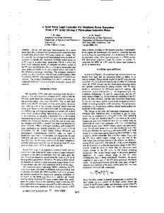
The control effects for the different DC/DC controllers under similar power references given by the ANN are shown in Figures 11 and 12. It can be observed that there is an obvious steady-state error in the feedback linearization method without augmentation (ANN + FL).The conventional PI controller (ANN + PI) tracks the ANN reference well under stable conditions or in the case of slow and uniform changes. However, a dynamic tracking overshoot exists under the condition of strong irradiance or when the irradiance changes rapidly. In other words, the ANN + FL and ANN + PI controllers cannot meet the demands of tracking the power reference under all conditions of the PV system. In order to illustrate the comparisons between each method distinctly, the output of each method divided by the ANN reference, are shown in Figure 12. It can be clearly observed that ANN + AFL is better than ANN + PI, and ANN + PI is better than ANN + FL, especially when avoiding the steady-state error.
Energies 2016, 9, 1005
14 of 25
Energies 2016, 9, 1005 The control effects for the different DC/DC controllers under similar power references given by 14 of 24
the ANN are shown in Figures 11 and 12.
(a)
(b) Figure 11. Output powers of PV systems with ANN and different DC/DC control strategies: (a)
Figure 11. Output powers of PV systems with ANN and different DC/DC control strategies: (a) Output Output power (overall); (b) Output power (detailed). power (overall); (b) Output power (detailed). Energies 2016, 9, 1005 15 of 25 104 102 100 98 96
104
94
ANN+PI ANN+FL ANN+AFL ANN Standard
92
100
90 88 0.1
96 0.598 0.6 0.602 0.604 0.606 0.608 0.61 0.2
0.3
0.4
0.5
0.6
0.7
0.8
0.9
1
Time(s)
Figure 12. Output of each method divided by the ANN reference.
Figure 12. Output of each method divided by the ANN reference. It can be observed that there is an obvious steady-state error in the feedback linearization method without augmentation (ANN + FL).The conventional PI controller (ANN + PI) tracks the ANN reference well under stable conditions or in the case of slow and uniform changes. However, a dynamic tracking overshoot exists under the condition of strong irradiance or when the irradiance changes rapidly. In other words, the ANN + FL and ANN + PI controllers cannot meet the demands of tracking the power reference under all conditions of the PV system. In order to illustrate the comparisons between each method distinctly, the output of each method divided by the ANN reference, are shown in Figure 12. It can be clearly observed that ANN + AFL is
dynamic tracking overshoot exists under the condition of strong irradiance or when the irradiance changes rapidly. In other words, the ANN + FL and ANN + PI controllers cannot meet the demands of tracking the power reference under all conditions of the PV system. In order to illustrate the comparisons between each method distinctly, the output of each method divided by the ANN reference, are shown in Figure 12. It can be clearly observed that ANN + AFL is Energies 2016, 9, 1005 15 of 24 better than ANN + PI, and ANN + PI is better than ANN + FL, especially when avoiding the steadystate error. Figures 13 13 andand 14 depict the performances of theof various MPPT Under these theseoperating operatingconditions, conditions, Figures 14 depict the performances the various controllers including the INC, fuzzy, and P&O controllers. It can be observed that each algorithm can MPPT controllers including the INC, fuzzy, and P&O controllers. It can be observed that each track the MPP effectively. algorithm can track the MPP effectively.
Energies 2016, 9, 1005
16 of 25
(a)
(b) Figure 13. 13. Output Output powers powers of of PV PV system system with with perturb-and-observe perturb-and-observe (P&O), (P&O), incremental incremental conductance conductance Figure (INC), fuzzy, and ANN + AFL methods: (a) Output power (overall); (b) Output power (detailed). (INC), fuzzy, and ANN + AFL methods: (a) Output power (overall); (b) Output power (detailed).
(b) Energies 2016, 9,Figure 1005 13. Output powers of PV system with perturb-and-observe (P&O), incremental conductance (INC), fuzzy, and ANN + AFL methods: (a) Output power (overall); (b) Output power (detailed).
16 of 24
14. Output power eachmethod method divided byby thethe ANN output power. FigureFigure 14. Output power ofofeach divided ANN output power.
In terms of the power-tracking process, under the stable condition or with slow and uniform
In changes, terms ofeach thealgorithm power-tracking process, under the stable condition or with slow and uniform demonstrates acceptable effects. Thealgorithm tracking operating point initially jumps, and then, it tracks the MPP slowly in the INC, changes, each demonstrates acceptable effects. and operating P&O methods, the irradiation changes This is because Thefuzzy, tracking pointwhen initially jumps, and then, itsuddenly. tracks the MPP slowly these in thethree INC, fuzzy, algorithms retain the duty cycles calculated at the last moment before the irradiation changed and P&O methods, when the irradiation changes suddenly. This is because these three algorithms suddenly. retain the duty cycles calculated at the last moment before the irradiation changed suddenly. It can be observed that the method presented in this paper (ANN + AFL) provides good dynamic It can be observed that the method in thisofpaper (ANN + AFL) provides good dynamic operation, faster convergence speed,presented less oscillations operating point around MPP, and more operation, faster convergence speed, less oscillations of operating point around MPP, and more effective tracking of global maxima under different conditions, than the INC, fuzzy, and P&O methods. In order illustrate the comparisons between each method distinctly, the output powers Energies to 2016, 9, 1005 17 of 25 of each method divided by the ANN output power, are shown in Figure 14. tracking of global under different conditions, than being the INC, fuzzy,than and 100% P&O at the It iseffective worth mentioning that,maxima in Figure 14, the reason for the ratio greater methods. beginning, is an error existing between the output power reference given by the ANN and the PV In order to illustrate the comparisons between each method distinctly, the output powers of each output power a lowby irradiance level. power, The error analysis remains methodat divided the ANN output are shown in Figure 14. consistent with that in Figure 6. The DC-link voltage and the current the for PVthe grid-connected inverter areatdepicted in It is worth mentioning that,output in Figure 14, the of reason ratio being greater than 100% the beginning, is an error existing between the output power reference given by V theand ANN the PV Figure 15. It can be observed that the DC-link voltage is maintained at 700 theand fluctuations are output power atrange a low irradiance within an acceptable about 10 level. V. The error analysis remains consistent with that in Figure 6. The DC-link voltage and the output current of the PV grid-connected inverter are depicted in The effectiveness of the MPPT method presented in this paper is shown in Figure 15b. The output Figure 15. It can be observed that the DC-link voltage is maintained at 700 V and the fluctuations are current within is consistent with the PV output characteristic curve in Figure 4. an acceptable range about 10 V. 720 715 710 705 700 695 690 685 680 0.1
0.2
0.3
0.4
0.5
Time(s)
0.6
(a)
Figure 15. Cont.
0.7
0.8
0.9
1
695 690 685 680 Energies 2016, 9, 1005
0.1
0.2
0.3
0.4
0.5
Time(s)
0.6
0.7
0.8
0.9
1
17 of 24
(a)
(b) Figure 15. DC-link voltage and inverter output current: (a) DC-link voltage; (b) Three-phase output
Figure 15. DC-link voltage and inverter output current: (a) DC-link voltage; (b) Three-phase current. output current. The effectiveness of the MPPT method presented in this paper is shown in Figure 15b. The output current 5.2. Simulation Case 2 is consistent with the PV output characteristic curve in Figure 4. 5.2. Simulation Case 2the performance of proposed method under extreme shading conditions, In order to evaluate different control methods and the algorithms which presented in simulation casepartial 1 are shading tested 18 under Energies 2016, 9,In 1005 of 25 order to evaluate performance of proposed method under extreme simulation case 2. different In this case, duration of simulation 0.6 s. The temperature maintained at conditions, controlthe methods and algorithms whichispresented in simulation case is 1 are tested a constant value of case 25 ◦ C2.inIn allthis sections. irradiance illustrated in under simulation case, The the temperature duration of and simulation is variations 0.6 s. Theare temperature is Figure 16. The changes every 0.05 from 0.15 s to 0.6 s as follows: maintained at airradiance constant value of 25 °C in all ssections. The temperature and irradiance variations are illustrated in Figure 16. The irradiance changes every 0.05 s from 0.15 s to 0.62s as follows: 0 s~0.15 s: The irradiance is maintained at a constant value of 500 W/m . 2 from 00.15 s~0.15 s: The irradiance is maintained constant of500 500W/m W/m22.. s~0.2 s: The irradiance is increasedat toa1000 W/mvalue 2 2. 0.15 s~0.2 s:s:The W/m 2. 0.2 s~0.25 Theirradiance irradianceisisincreased decreasedtoto1000 200 W/m W/m2from from500 1000 W/m 0.2 s~0.25 s: The irradiance is decreased to 200 W/m2 2from 1000 W/m22. 0.25 s~0.3 s: The irradiance is increased to 900 W/m from 200 W/m . 0.25 s~0.3 s: The irradiance is increased to 900 W/m2 from 200 W/m2. 2 2 from 0.3 s~0.35 s: The irradiance is decreased to 300 W/m 900 W/m . 0.3s~0.35 s: The irradiance is decreased to 300 W/m2 from 900 W/m2. 2 2 0.35 s~0.4 s: The irradiance is increased to 800 W/m from 300 W/m . 0.35s~0.4 s: The irradiance is increased to 800 W/m2 from 300 W/m2. 2 2 0.4 s~0.45s:s:The Theirradiance irradianceisisdecreased decreasedtoto400 400W/m W/m from 800 W/m . 2 from 2. 0.4s~0.45 800 W/m 2 from 400 W/m2 . 0.45 s~0.5 s: The irradiance is increased to 700 W/m 0.45s~0.5 s: The irradiance is increased to 700 W/m2 from 400 W/m2. 2 from 700 W/m2 . 0.5 s~0.55s:s:The Theirradiance irradianceisisdecreased decreasedtoto500 500W/m W/m 2 from 0.5s~0.55 700 W/m2. 2 2 2. 2 . 0.55 s~0.6s:s:The Theirradiance irradianceisisincreased increasedtoto600 600W/m W/mfrom from 500 W/m 0.55s~0.6 500 W/m
Figure 16. Temperature Temperature and irradiance variations in case 2.
The analysis is similar to that of simulation case 1. The control effects with different DC/DC controllers are shown in Figure 17. Speed, accuracy, reliability, power loss, and oscillation during the tracking period are the main factors monitored in the evaluation and validation processes.
Energies 2016, 9, 1005
18 of 24
Figure 16. Temperature and irradiance variations in case 2.
The analysis analysis is is similar similar to to that that of of simulation simulation case case1.1. The The control control effects effectswith withdifferent differentDC/DC DC/DC controllers are shown in Figure 17. Speed, accuracy, reliability, power loss, and oscillation during controllers are shown reliability, power loss, and oscillation during the tracking period period are are the the main main factors factors monitored monitored in in the the evaluation evaluationand andvalidation validationprocesses. processes.
(a)
19 of 25
Percent of Tracking ANN Instruction(%)
Energies 2016, 9, 1005
(b) Figure 17. 17. Output and different DC/DC control strategies: (a) Figure Outputpowers powersofofthe thePV PVsystem systemwith withANN ANN and different DC/DC control strategies: Output power (overall); (b) Output of each method divided by ANN reference. (a) Output power (overall); (b) Output of each method divided by ANN reference.
ystem Output Power(kW)
It can be observed from Figure 17 that the ANN + PI controller can track the MPP with a small It can be observed from Figure 17 that the ANN + PI controller can track the MPP with a small steady-state error, but it cannot provide good dynamic operation when the irradiation changes steady-state error, but it cannot provide good dynamic operation when the irradiation changes suddenly. The ANN + FL controller can provide good dynamic operation; however, it demonstrates suddenly. The ANN + FL controller can provide good dynamic operation; however, it demonstrates an obvious steady-state error. The MPP in this condition can be tracked by all methods proposed in an obvious steady-state error. The MPP in this condition can be tracked by all methods proposed in Figure 17. The proposed ANN + AFL technique however tracked the MPP in a much shorter time Figure 17. The proposed ANN + AFL technique however tracked the MPP in a much shorter time and and with fewer oscillations during the tracking period than other methods. with fewer oscillations during the tracking period than other methods. In order to illustrate the comparisons between each method distinctly, the output of each method In order to illustrate the comparisons between each method distinctly, the output of each method divided by the ANN reference, are shown in Figure 17b. It can be clearly observed that the control divided by the ANN reference, are shown in Figure 17b. It can be clearly observed that the control effect of ANN + AFL is better than ANN + PI, and ANN + PI is better than ANN + FL, especially when effect of ANN + AFL is better than ANN + PI, and ANN + PI is better than ANN + FL, especially when avoiding the steady-state error. avoiding the steady-state error. Figure 18 depicts the performances of the MPPT controllers including the INC, fuzzy, and P&O Figure 18 depicts the performances of the MPPT controllers including the INC, fuzzy, and P&O controllers. It can be observed that each algorithm can track the MPP effectively. However, most of controllers. It can be observed that each algorithm can track the MPP effectively. However, most of these methods suffer from slow convergence time or low efficiency. these methods suffer from slow convergence time or low efficiency.
PV System Output Power(kW)
divided by the ANN reference, are shown in Figure 17b. It can be clearly observed that the control effect of ANN + AFL is better than ANN + PI, and ANN + PI is better than ANN + FL, especially when avoiding the steady-state error. Figure 18 depicts the performances of the MPPT controllers including the INC, fuzzy, and P&O controllers. It1005 can be observed that each algorithm can track the MPP effectively. However, most Energies 2016, 9, 19 ofof 24 these methods suffer from slow convergence time or low efficiency.
Energies 2016, 9, 1005
20 of 25
(a)
(b) Figure 18. P&O, INC, fuzzy, and ANN + AFL methods: (a) Figure 18. Output Outputpowers powersofofthe thePV PVsystem systemwith with P&O, INC, fuzzy, and ANN + AFL methods: Output power (overall); (b) (b) Output power (detailed). (a) Output power (overall); Output power (detailed).
As shown, the fuzzy and P&O method track the MPP within around half the tracking time of As shown, the fuzzy and P&O method track the MPP within around half the tracking time of the INC algorithm. The proposed ANN + AFL algorithm tracks the MPP within a very short time and the INC algorithm. The proposed ANN + AFL algorithm tracks the MPP within a very short time only little power loss. In order to illustrate the comparisons between each method distinctly, the and only little power loss. In order to illustrate the comparisons between each method distinctly, the output powers of each method divided by the ANN output power, are shown in Figure 18b. output powers of each method divided by the ANN output power, are shown in Figure 18b. It is worth mentioning that, in Figure 18b, the reason for the ratio being greater than 100% at the It is worth mentioning that, in Figure 18b, the reason for the ratio being greater than 100% at the irradiance switching point, is an error existing between the output power reference given by the ANN irradiance switching point, is an error existing between the output power reference given by the ANN and the PV output power at a low irradiance level. The error analysis remains consistent with that in and the PV output power at a low irradiance level. The error analysis remains consistent with that in Figure 6. Figure 6. It can be observed that, even under conditions when the irradiation changes rapidly, the method It can be observed that, even under conditions when the irradiation changes rapidly, the method presented in this paper (ANN + AFL) can provide good dynamic operation, faster convergence speed, presented in this paper (ANN + AFL) can provide good dynamic operation, faster convergence speed, less oscillations of operating point around MPP, and more effective tracking of global maxima under less oscillations of operating point around MPP, and more effective tracking of global maxima under different conditions, than the INC, fuzzy, and P&O methods. An important outcome resulting from different conditions, than the INC, fuzzy, and P&O methods. An important outcome resulting from the application of the ANN + AFL technique for MPPT is the reduction in power loss during both the the application of the ANN + AFL technique for MPPT is the reduction in power loss during both the tracking and steady-state periods. tracking and steady-state periods. At the same time, the DC-link voltage is maintained at 700 V and the output current of the PV as shown in Figure 19, is consistent with the PV output characteristic curve in Figure 4.
Figure 6. It can be observed that, even under conditions when the irradiation changes rapidly, the method presented in this paper (ANN + AFL) can provide good dynamic operation, faster convergence speed, less oscillations of operating point around MPP, and more effective tracking of global maxima under different conditions, than the INC, fuzzy, and P&O methods. An important outcome resulting from Energies 2016, 9, 1005 20 of 24 the application of the ANN + AFL technique for MPPT is the reduction in power loss during both the tracking and steady-state periods. At the the same same time, time,the theDC-link DC-linkvoltage voltageisismaintained maintainedatat700 700V V and output current At and thethe output current of of thethe PVPV as as shown in Figure is consistent with output characteristic curve in Figure shown in Figure 19,19, is consistent with thethe PVPV output characteristic curve in Figure 4. 4.
Energies 2016, 9, 1005
21 of 25
(a)
60
a phase current b phase current c phase current upper envelope lower envelope
Three phase current(A)
45 30 15 0 -15 -30 -45 -60 0.1
0.15
0.2
0.25
0.3
0.35
Time(s)
0.4
0.45
0.5
0.55
0.6
(b) Figure voltage andand inverter output current: (a) DC-link voltage; (b) Three-phase output Figure 19. 19. DC-link DC-link voltage inverter output current: (a) DC-link voltage; (b) Three-phase current. output current.
6. 6. Conclusions Conclusions A nonlinear control A detailed detailed analysis analysis and and design design of of an an MPPT MPPT solution solution based based on on ANN ANN and and the the nonlinear control theory was introduced in this paper. This solution aimed at performing fast MPPT in PV PV systems. systems. theory was introduced in this paper. This solution aimed at performing fast MPPT in In the nonlinear nonlinear characteristics temperature In terms terms of of the characteristics of of PV PV systems, systems, which which were were based based on on the the temperature and irradiation, an ANN was utilized to deliver the reference power to the DC/DC boost and irradiation, an ANN was utilized to deliver the reference power to the DC/DC boostconverter. converter. Under extremely low lowirradiance irradiancelevels, levels,the the relative error percentage lesser Training Under extremely relative error percentage waswas lesser thanthan 4%. 4%. Training data data showed a trifling relative error percentage lesser than 0.5% in the normal irradiance range showed a trifling relative error percentage lesser than 0.5% in the normal irradiance range between 2 2 and 2 . W/m2. between W/m 1000 200 W/m200 1000and W/m After After the the reference reference power power was was supplied supplied by by the the ANN, ANN, an an AFL AFL control control strategy strategy was was proposed proposed for for the DC/DC boost converter, according to the non-linear control theory. the DC/DC boost converter, according to the non-linear control theory. The ANN + + AFL ANN + + PI, The control control effect effect of of ANN AFL was was better better than than that that of of ANN PI, which which was was better better than than that that of of ANN ANN ++ FL, FL, especially especially on on avoiding avoiding steady-state steady-state errors. errors. The The proposed proposed ANN ANN ++ AFL AFL control control strategy strategy showed good dynamic dynamic performance performancewith withonly onlyaatrifling triflingsteady-state steady-stateerror error while tracking MPP showed aa good while tracking thethe MPP of of the PV units even with rapid changes in irradiation. It demonstrated precise and fast tracking of the MPP, better than the ANN + PI and ANN + FL methods. The control strategy of the inverter was designed with full consideration of the requirements of the PV system operating in the grid-connected mode. The results showed that, under the gridconnected mode, the DC-link voltage was maintained at 700 V and the output current of the PV
Energies 2016, 9, 1005
21 of 24
the PV units even with rapid changes in irradiation. It demonstrated precise and fast tracking of the MPP, better than the ANN + PI and ANN + FL methods. The control strategy of the inverter was designed with full consideration of the requirements of the PV system operating in the grid-connected mode. The results showed that, under the grid-connected mode, the DC-link voltage was maintained at 700 V and the output current of the PV system was consistent with the PV output characteristic curve. The system was simulated using MATLAB/Simulink. From the simulation results, it could be observed that, an important outcome resulting from the application of the ANN + AFL technique for MPPT is the reduction in power loss during both the tracking and steady-state periods. With rapid changes in irradiation and temperature, the method presented in this paper (ANN + AFL) could provide good dynamic operation, faster convergence speed, trifling steady-state error, and fewer oscillations of the operating point around the MPP. Acknowledgments: This paper was supported by the National Natural Science Foundation of China (51377007) and by the Specialized Research Fund for the Doctoral Program of Higher Education in China (20131102130006). Author Contributions: All authors contributed equally to this work. Conflicts of Interest: The authors declare no conflict of interest.
Appendix A. Nonlinearity Control Theory and Parameter Analysis in Third-Order Systems Appendix A.1. Some Definitions in Nonlinearity Control Theory 1.
Vector field: Given a subset S in Rn , a vector field is represented by a vector-valued function V: S→Rn in standard Cartesian coordinates (x1 , . . . , xn ). If each component of V is continuous, then V is a continuous vector field, and more generally, V is a Ck vector field if each component of V is k times continuously differentiable. A vector field can be visualized by assigning vectors to individual points within an n-dimensional space. A vector field defines a unique dynamical system described as a differential equation: •
x = f (x)
2.
(A1)
i.e., a vector field f, with initial condition x0 , determines an integral curve t→(x1 (t), . . . , xn (t)), which is a solution to Equation (A1) such that x(0) = x0 . Lie derivative: If f is a smooth vector field on U and h is a smooth function on U, then, f (h) is a smooth function on U defined by: n
f (h(x)) =
∑ fi (x)(
i =1
∂h(x) ) ∂xi
(A2)
A vector field can be interpreted as an operator mapping the function h onto the function f (h). The function f (h) is called the Lie derivative of the function h along the vector field f ; it is usually denoted as Lf h, which is a more convenient notation for repeated operations: L f1 L f2 L f3 . . . L f i h = f 1 ( f 2 ( f 3 (. . . f i (h) . . .))) Repeated Lie derivatives along the same vector field f are denoted as Lkf h = L f (Lkf −1 h), L0f h = h. The Lie derivative Lf h of a smooth function h along a vector field f is also denoted by hdh, f i. 3.
Lie bracket: If f and g are smooth vector fields on U and h is a smooth function on U, then, [f, g](h) is a smooth function on U defined by:
[ f , g](h) = f ( g(h)) − g( f (h)) = L f Lg h − Lg L f h
(A3)
Energies 2016, 9, 1005
22 of 24
The Lie bracket [f, g] of two vector fields f and g is also denoted by ad f g. [f, g] is a vector field. Repeated Lie brackets are denoted as adif g = ad f ( adif−1 g), ad0f g = g. Appendix A.2. Multi-Input Feedback Linearization Theorem •
m
The nonlinear system x = f (x) + ∑ gi (x)ui = f (x) + G (x)u, x ∈ Rn is locally feedback i =1
linearizable, i.e., locally transformable in V 0 , a neighborhood of the origin contained in U0 , into a linear controllable system in the Brunovsky controller form by means of: 1.
a nonsingular state feedback: u = K (x) + β(x)v, K (0) = 0
2.
where K(x) is a smooth function from V 0 onto Rn , β(x) is an m × m matrix with smooth entries, nonsingular in V 0 a local diffeomorphism in V 0 : z = T (x), T (0) = 0, if, and only if, in U0 : j
1.
Θl = Span{ ad f gi : 1 ≤ i ≤ m, 0 ≤ j ≤ l }, 0 ≤ l ≤ n − 2, is involutive and of constant rank.
2.
Rank Θn−1 = n Rank Gn −1 = n.
Appendix B. Simulation Parameters Simulation Parameters Output power under the STC = 21.96 kW, Carrier frequency in VMPPT PWM generator = 5 kHz and in grid-side controller = 10 kHz, Boost converter parameters: L = 0.5 mH, Cin = 330 µF, Cdc = 630 µF, √ Udc = 700 V, ωo = 1/ LCin = 2.46 × 10³ , ωn = 2ωo = 4.92 × 10³ , ξ = 5, k = 2, k1 = ωn3 = 1.2 × 10¹¹ , k2 = ωn2 (2ξ + 1) = 2.67 × 10⁸ , k3 = ωn (2ξ + 1) = 5.42 × 10⁴ , PI coefficients in the grid-side controller: KpVdc = 50, KiVdc = 3, KpId = 10, KiId = 5, KpIq = 10, KiIq = 5. References 1. 2. 3. 4. 5. 6. 7. 8. 9. 10. 11. 12.
Renewable Energy Policy Network for the 21st Century (REN21). Renewables 2010; Global Status Report; REN21 Secretariat: Paris, France, 2010. International Energy Agency (IEA). Technology Roadmap Solar, Photovoltaic Energy; IEA: Paris, France, 2010. Kish, G.J.; Lee, J.J.; Lehn, P.W. Modelling and control of photovoltaic panels utilising the incremental conductance method for maximum power point tracking. IET Renew. Power Gener. 2012, 6, 259–266. [CrossRef] Femia, N.; Petrone, G.; Spagnuolo, G.; Vitelli, M. A technique for improving P&O MPPT performances of double-stage grid-connected photovoltaic systems. IEEE Trans. Ind. Electron. 2009, 56, 4473–4482. Esram, T.; Chapman, P.L. Comparison of photovoltaic array maximum power point tracking techniques. IEEE Trans. Energy Convers. 2007, 22, 439–449. [CrossRef] Gonzalez, D.; Ramos-Paja, C.A.; Petrone, G. Automated procedure for calculating the controller parameters in photovoltaic dc/dc converters. Int. Rev. Electr. Eng. 2011, 6, 3027–3040. Adinolfi, G.; Femia, N.; Petrone, G.; Spagnuolo, G.; Vitelli, M. Design of dc/dc converters for DMPPT PV applications based on the concept of energetic efficiency. J. Sol. Energy Eng. 2010, 132. [CrossRef] Rezvani, A.; Gandomkar, M.; Izadbakhsh, M.; Ahmadi, A. Environmental/economic scheduling of a micro-grid with renewable energy resources. J. Clean. Prod. 2015, 87, 216–226. [CrossRef] Hohm, D.P.; Ropp, M.E. Comparative study of maximum power point tracking algorithms. Prog. Photovolt. Res. Appl. 2003, 11, 47–62. [CrossRef] Salas, V.; Olias, E.; Barrado, A.; Lazaro, A. Review of the maximum power point tracking algorithms for stand-alone photovoltaic systems. Sol. Energy Mater. Sol. Cells 2006, 90, 1555–1578. [CrossRef] Ahmed, J.; Salam, Z. An improved perturb and observe (P&O) maximum power point tracking (MPPT) algorithm for higher efficiency. Appl. Energy 2015, 150, 97–108. Piegari, L.; Rizzo, R. Adaptive perturb and observe algorithm for photovoltaic maximum power point tracking. IET Renew. Power Gener. 2010, 4, 317–328. [CrossRef]
Energies 2016, 9, 1005
13. 14. 15.
16. 17. 18.
19. 20.
21.
22. 23. 24.
25. 26.
27.
28.
29. 30.
31. 32. 33. 34.
23 of 24
Mamarelis, E.; Petrone, G.; Spagnuolo, G. A two-steps algorithm improving the P&O steady state MPPT efficiency. Appl. Energy 2014, 113, 414–421. Hussein, K.H.; Muta, I.; Hoshino, T.; Osakada, M. Maximum photovoltaic power tracking: An algorithm for rapidly changing atmospheric conditions. IEEE Proc. Gener. Transm. Distrib. 1995, 142, 59–64. [CrossRef] Hsieh, G.C.; Chen, H.L.; Chen, Y.; Tsai, C.M.; Shyu, S.S. Variable frequency controlled incremental conductance derived MPPT photovoltaic stand-along DC bus system. In Proceedings of the 23th Annual IEEE Applied Power Electronics Conference and Exposition, Austin, TX, USA, 24–28 February 2008. Qiang, M.; Mingwei, S.; Liying, L.; Guerrero, J.M. A novel improved variable step-size incremental-resistance MPPT method for PV systems. IEEE Trans. Ind. Electron. 2011, 58, 2427–2434. Algazar, M.M.; Al-Monier, H.; EL-halim, H.A.; Salem, M.E.E.K. Maximum power point tracking using fuzzy logic control. Int. J. Electr. Power Energy Syst. 2012, 39, 21–28. [CrossRef] Liu, L.; Liu, C.; Wang, J.; Kong, Y. Simulation and hardware implementation of a hill-climbing modified fuzzy-logic for maximum power point tracking with direct control method using boost converter. J. Vib. Control 2015, 21, 335–342. [CrossRef] Chiu, C.S.; Ouyang, Y.L. Robust maximum power tracking control of uncertain photovoltaic systems: A unified T-S fuzzy model-based approach. IEEE Trans. Control Syst. Technol. 2011, 19, 1516–1526. [CrossRef] Khaldi, N.; Mahmoudi, H.; Zazi, M.; Barradi, Y. The MPPT control of PV system by using neural networks based on Newton Raphson method. In Proceedings of the 2014 International Renewable and Sustainable Energy Conference (IRSEC), Quarzazate, Morocco, 17–19 October 2014. Singh, M.D.; Shine, V.J.; Janamala, V. Application of artificial neural networks in optimizing MPPT control for standalone solar PV system. In Proceedings of the 2014 International Conference on Contemporary Computing and Informatics (IC3I), Mysore, India, 27–29 November 2014. Elobaid, L.M.; Abdelsalam, A.K.; Zakzouk, E.E. Artificial neural network-based photovoltaic maximum power point tracking techniques: A survey. IET Renew. Power Gener. 2015, 9, 1043–1063. [CrossRef] Valencia, P.A.O.; Ramos-Paja, C.A. Sliding-mode controller for maximum power point tracking in grid-connected photovoltaic systems. Energies 2015, 8, 12363–12387. [CrossRef] Bianconi, E.; Calvente, J.; Giral, R.; Mamarelis, E.; Petrone, G.; Ramos-paja, C.A.; Spagnuolo, G.; Vitelli, M. A fast current-based MPPT technique employing sliding mode control. IEEE Trans. Ind. Electron. 2013, 60, 1168–1178. [CrossRef] Gonzalez Montoya, D.; Ramos-Paja, C.A.; Giral, R. Improved design of sliding mode controllers based on the requirements of MPPT techniques. IEEE Trans. Power Electron. 2015, 31, 235–247. [CrossRef] Liu, Y.H.; Huang, S.C.; Huang, J.W.; Liang, W.C. A particle swarm optimization-based maximum power point tracking algorithm for PV systems operating under partially shaded conditions. IEEE Trans. Energy Convers. 2012, 27, 1027–1035. [CrossRef] Renaudineau, H.; Donatantonio, F.; Fontchastagner, J.; Petrone, G.; Spagnuolo, G.; Martin, J.-P.; Pierfederici, S. A PSO-Based Global MPPT Technique for Distributed PV Power Generation. IEEE Trans. Ind. Electron. 2015, 62, 1047–1058. [CrossRef] Benyoucef, A.S.; Chouder, A.; Kara, K.; Silvestre, S.; Sahed, O.A. Artificial bee colony based algorithm for maximum power point tracking (MPPT) for PV systems operating under partial shaded conditions. Appl. Soft Comput. 2015, 32, 38–48. [CrossRef] Trejos, A.; Gonzalez, D.; Ramos-Paja, C.A. Modeling of step-up grid-connected photovoltaic systems for control purposes. Energies 2012, 5, 1900–1926. [CrossRef] Punitha, K.; Devaraj, D.; Sakthivel, S. Artificial neural network based modified incremental conductance algorithm for maximum power point tracking in photovoltaic system under partial shading conditions. Energy 2013, 62, 330–340. [CrossRef] Rezvani, A.; Gandomkar, M. Modeling and control of grid connected intelligent hybrid photovoltaic system using new hybrid fuzzy-neural method. Sol. Energy 2016, 127, 1–18. [CrossRef] Mutlag, A.H.; Mohamed, A.; Shareef, H. A nature-inspired optimization-based optimum fuzzy logic photovoltaic inverter controller utilizing an eZdsp F28335 Board. Energies 2016, 9. [CrossRef] Shiau, J.; Wei, Y.; Lee, M. Fuzzy controller for a voltage-regulated solar-powered MPPT system for hybrid power system application. Energies 2015, 8, 3292–3312. [CrossRef] Bhatnagar, P.; Nema, R.K. Maximum power point tracking control techniques: State-of-the-art in photovoltaic applications. Renew. Sustain. Energy Rev. 2013, 23, 224–241. [CrossRef]
Energies 2016, 9, 1005
35. 36. 37. 38.
39. 40.
41. 42.
43. 44.
45. 46.
24 of 24
Ahmed, J.; Salam, Z. A critical evaluation on maximum power point tracking methods for partial shading in PV systems. Renew. Sustain. Energy Rev. 2015, 47, 933–953. [CrossRef] Manganiello, P.; Ricco, M.; Petrone, G.; Monmasson, E.; Spagnuolo, G. Optimization of perturbative PV MPPT methods through online system identification. IEEE Trans. Ind. Electron. 2014, 61, 6812–6821. [CrossRef] Mamarelis, E.; Petrone, G.; Spagnuolo, G. A hybrid digital-analog sliding mode controller for photovoltaic applications. IEEE Trans. Ind. Inf. 2103, 9, 1094–1103. [CrossRef] Haroun, R.; Aroudi, A.E.; Cid-Pastor, A.; Garcia, G.; Olalla, C.; Martinez-Salamero, L. Impedance matching in photovoltaic systems using cascaded boost converters and sliding-mode control. IEEE Trans. Power Electron. 2015, 30, 3185–3199. [CrossRef] Erickson, R.W.; Maksimovic, D. Fundamentals of Power Electronics, 2nd ed.; Springer: Berlin, Germany, 2007. Hossein, A.M.; Hossein, M. Improving the performance of a nonlinear boiler-turbine unit via bifurcation control of external disturbances: A comparison between sliding mode and feedback linearization control approaches. Nonlinear Dyn. 2016, 85, 229–243. Xibei, D.; Alok, S. Hydropower plant frequency control via feedback linearization and sliding mode control. J. Dyn. Syst. Meas. Control 2016, 138. [CrossRef] Francesco, A.; Maurizio, C.; Marcello, P.; Antonino, S. Input-output feedback linearization control with on-line MRAS-based inductor resistance estimation of linear induction motors including the dynamic end effects. IEEE Trans. Ind. Appl. 2016, 52, 254–266. Dannehl, J.; Wessels, C.; Fuchs, F.W. Limitation of voltage-oriented PI current control of grid-connected PWM rectifier with LCL filters. IEEE Trans. Ind. Electron. 2009, 56, 380–388. [CrossRef] Dannehl, J.; Fuchs, F.W.; Hansen, S.; Thogersen, P.B. Investigation of active damping approaches for PI-based current control of grid-connected pulse width modulation converter with LCL filters. IEEE Trans. Ind. Appl. 2010, 46, 1509–1517. [CrossRef] Dannehl, J.; Fuchs, F.W.; Thogersen, P.B. PI state current control of grid-connected PWM converters with LCL filters. IEEE Trans. Power Electron. 2010, 25, 2320–2330. [CrossRef] Hwang, T.S.; Park, S.Y. A seamless control strategy of a distributed generation inverter for the critical load safety under strict grid disturbances. IEEE Trans. Power Electron. 2013, 28, 4780–4790. [CrossRef] © 2016 by the authors; licensee MDPI, Basel, Switzerland. This article is an open access article distributed under the terms and conditions of the Creative Commons Attribution (CC-BY) license (http://creativecommons.org/licenses/by/4.0/).