G.S.V.S. Sivaram, Samuel Thomas, Hynek Hermansky. Center for Language and ... Index Terms: Speaker Verification, Neural Networks, Factor. Analysis. 1.
Mixture of Auto-Associative Neural Networks for Speaker Verification G.S.V.S. Sivaram, Samuel Thomas, Hynek Hermansky Center for Language and Speech Processing Department of Electrical and Computer Engineering The Johns Hopkins University Baltimore, USA {sivaram,samuel,hynek}@jhu.edu
Abstract The paper introduces a mixture of auto-associative neural networks for speaker verification. A new objective function based on posterior probabilities of phoneme classes is used for training the mixture. This objective function allows each component of the mixture to model part of the acoustic space corresponding to a broad phonetic class. This paper also proposes how factor analysis can be applied in this setting. The proposed techniques show promising results on a subset of NIST08 speaker recognition evaluation (SRE) and yield about 10% relative improvement when combined with the state-of-the-art Gaussian Mixture Model i-vector system. Index Terms: Speaker Verification, Neural Networks, Factor Analysis
1. Introduction Auto-Associative Neural Networks (AANNs) have been recently proposed as an alternative to Gaussian Mixture Models (GMMs) for modeling the distribution of data [1]. An AANN is a feed-forward neural network trained to reconstruct its input at its output through a hidden compression layer. AANNs have several advantages compared to the GMMs - they relax the assumption of feature vectors to be locally normal and can capture higher order moments. In [1, 2], AANNs have been used instead of GMMs for speaker verification. However, these systems do not meet the performance of GMM based systems. This could be due to the limitation of a single AANN being used for modeling the entire acoustic space. This paper introduces a mixture of AANNs for speaker verification. The mixture consists of several AANNs tied using posterior probabilities of various broad phoneme classes. Since AANN is not a density model, these posteriors are obtained from a separate multilayer perceptron (MLP) classifier trained to estimate posterior probabilities of phoneme classes. This paper also proposes how the adaptation parameters of the mixture of AANNs can be modeled in a lower dimensional subspace using factor analysis. The remainder of the paper is organized as follows. In section 2, we summarize the earlier work on AANNs for speaker verification where a single AANN is used to characterize a This research was funded by the Office of the Director of National Intelligence (ODNI), Intelligence Advanced Research Projects Activity (IARPA), through the Army Research Laboratory (ARL). All statements of fact, opinion or conclusions contained herein are those of the authors and should not be construed as representing the official views or policies of IARPA, the ODNI, or the U.S. Government.
speaker. Section 3 describes the proposed mixture of AANNs. Experimental results are presented in Section 4. The subspace modeling of adaptation parameters of the proposed model is described along with results in section 5. The paper concludes with a discussion on future work in Section 6.
2. Auto-Associative Neural Networks 2.1. Modeling Data with AANNs AANNs are feed-forward neural networks with several layers trained to reconstruct the input at its output through a hidden compression layer [3]. Five layer AANNs are used in all our experiments. This architecture consists of three non-linear hidden layers between the linear input and output layers. The second hidden layer contains fewer nodes than the input layer, and is known as the compression layer. For an input vector x, the network produces an output ˆ (x, W) which depends both on the input x and the parameters x W of the network (the set of weights and biases). For simplicity, ˆ (W). While training the netwe denote the network output as x work, the parameters W of the network are typically adjusted to minimize the average squared error cost between the input ˆ (W) over the training data as in (1). The x and the output x network is trained using the error back-propagation algorithm. ˆ ˜ ˆ (W)k2 . min E kx − x (1) {W}
Once this network is well trained, the average reconstruction error of input vectors that are drawn from the distribution of the training data will be small compared to vectors drawn from a different distributions [1]. The reconstruction error can be linked to the likelihood by modeling the likelihood of input x under the AANN model W as ˆ (W)k2 ). p (x; W) ∝ exp(−kx − x Assuming the data to be i.i.d, minimizing the average reconstruction error of training data with respect to W is same as maximizing the likelihood of the data. 2.2. Speaker Verification using AANN In previously proposed AANN based speaker verification systems [1, 2], a single AANN is trained on large amounts of data containing multiple speakers. This AANN captures speaker independent distribution of the input acoustic feature vectors, and is used as the universal background model (UBM). For each speaker in the enrollment set, a speaker-specific AANN model
Acoustic Features A1
Broad Class Posteriors Test Utterance
UBM Model A4
UBM average reconstruction error
A3 A2
A5 Decision Logic
MLP Acoustic Features
Speaker Model A4
A1 A3 Acoustic Features
Decision
A2
A5
Speaker average reconstruction error
Component AANNs
Figure 1: Block schematic of the proposed mixture of AANNs based speaker verification system.
is obtained by retraining the entire UBM-AANN using the enrollment data. During the test phase, the average reconstruction error of the test data is computed under both UBM-AANN model and the claimed speaker AANN model. The final score for each test utterance is computed as the difference between these average reconstruction errors. In the ideal case, if the claim is verified, the average reconstruction error of the test data will be larger under the UBM-AANN model than the claimed speaker AANN model, and vice versa. This approach is similar to conventional UBM-GMM techniques [4] except for the maximum a posteriori probability (MAP) adaptation to obtain speaker specific model. Unlike in the MAP adaptation of UBM-GMM, in which only those components that are well represented in the adaptation data get significantly modified, there is no such an ability available during the adaptation of UBM-AANN. To address this issue, we introduce a mixture of AANNs as described in the following section.
3. Mixture of AANNs We propose a mixture of AANNs composed of several independent AANNs, each modeling only part of the acoustic vector space. The means by which a given frame of the data is assigned to an appropriate AANN is by using a separate multilayer perceptron (MLP) trained on labeled data to estimate the posterior probability of the underlying speech sound class. Thus, in this proposed scheme, the features that describe the speaker identity for training the mixture of AANNs are no longer required to provide the information about the underlying speech class as this information is now provided by the MLP. This may prove useful in certain applications. The following objective function is minimized for training the mixture " c # X 2 ˆ (Wj )k , P (Cj /x) kx − x min E (2) {W1 ,...,Wc }
j=1
where c denotes the number of mixture components or number of broad phoneme classes, and the set Wj consists of parameters of the j th AANN of the mixture. P (Cj /x) is the posterior probability of j th broad phonetic class Cj given x. The above objective function can be simplified as c X j=1
ˆ ˜ ˆ (Wj )k2 . min E P (Cj /x) kx − x
{Wj }
(3)
Since (2) can be simplified as (3), each AANN component of the mixture can be independently trained using the backpropagation algorithm as in (1). The only difference in training j th AANN component is that the corresponding error vector needs to be weighted by P (Cj /x) in the back-propagation algorithm. This allows each AANN component to model the distribution of feature vectors belonging to a particular broad phonetic class. 3.1. Speaker Verification using Mixture of AANNs A mixture of AANNs with five broad phoneme classes namely - vowels, fricatives, nasals, stops and silence trained on large amounts of data is used as a UBM. Once the UBM has been trained, the next step is to adapt it using the enrollment data. Since the amount of adaptation data is limited, we retrain only the last layer weights of each AANN component. This procedure is referred as the adaptation of the mixture throughout this paper. We also restrict the number of nodes of the third hidden layer to the size of the output layer to limit the number of adaptation parameters. The average reconstruction error of data D = {x1 , . . . , xn } under a mixture model is given by
e (D; W1 , . . . , Wc ) =
n P c P
P (Cj /xi ) kxi − xˆi (Wj )k2
i=1 j=1
n
.
The block schematic of the proposed framework is shown in Fig. 1.
4. Speaker Verification System 4.1. Acoustic Features The acoustic features used in our experiments are 39 dimensional FDLP features [5]. In this technique, sub-band temporal envelopes of speech are first estimated in narrow sub-bands (96 linear bands). These sub-band envelopes are then gain normalized to remove reverberation and channel artifacts. After normalization, the frequency axis is warped to the mel scale. We use 37 Mel bands in the frequency range of 125-3800 Hz to derive a gain normalized mel scale energy representation of speech similar to the mel spectogram obtained in conventional MFCC feature extraction. These mel band energies are converted to cepstral coefficients by using a log operation followed
(4)
by DCT. We use 13 cepstral coefficients along with derivative and acceleration components yielding 39 dimensional features. 4.2. Mixture of AANNs System As described in Sec. 3.1, we train a mixture of AANNs with five components on sufficiently large amounts of data to serve as UBM. Gender specific UBMs are trained on a telephone development data set consisting of audio from the NIST 2004 speaker recognition database, the Switchboard II Phase III corpora and the NIST 2006 speaker recognition database. We use only 400 male and 400 female utterances each corresponding to about 17 hours of speech. Posteriors to train the UBM are derived from an MLP trained on 300 hours of conversational telephone speech (CTS) [6]. The 45 phoneme posteriors are combined appropriately to obtain 5 broad phonetic class posteriors corresponding to vowels, fricatives, plosives, nasals and silence. Each AANN component of the UBM has a linear input and a linear output layer along with three nonlinear (tanh nonlinearity) hidden layers. Both input and output layers have 39 nodes corresponding to the dimensionality of the input FDLP features. We use 160 nodes in the first hidden layer, 20 nodes in the compression layer and 39 nodes in the third hidden layer. Speaker specific models are obtained by adapting (retraining) only the last layer weights (39×39 parameters) of each AANN component. Once the UBMs and speaker models have been trained, a score for a trial is computed as difference between the average reconstruction error (given by (4)) values of test utterance under the UBM model and the claimed model. 4.3. Results As a baseline, we train a gender independent UBM-GMM system with 1024 components on FDLP features (Sec. 4.1). The UBM-GMM is trained using the entire development data described in above section. The speaker specific GMM models are obtained by MAP adapting the UBM-GMM with a relevance factor 16. As a second baseline, we train gender specific AANN systems as described in Sec. 2.2. These systems use 160 nodes in both the second and fourth hidden layers and 20 nodes in the compression layer. The UBMs are trained using the same development data that is used for training the mixture of AANNs (see Sec. 4.2). Table 1: Performance in terms of Min DCF (×103 ) and EER (%) in parentheses on different NIST-08 conditions System GMM (1024 comp.) Baseline AANN Mixture of AANNs Mixture of AANNs + GMM
C6 84.4 (17.3) 88.3 ( 28.7) 86.7 (22.5)
C7 60.8 (11.7) 75.9 (20.6) 60.4 (11.8)
C8 69.1 (14.3) 77.0 (25.7) 57.3 (12.8)
81.3 (16.4)
51.9 (10.9)
54.4 (11.4)
results to the conventional GMM system. The score combination (equal weighting) of GMM baseline and the proposed system further improves the performance. However, state-ofthe-art GMM systems use factor analysis to obtain much better gains. In the next section, we describe how such techniques can be developed for the current framework.
5. Subspace Modeling of Mixture of AANNs In a recent work, factor analysis of GMMs has been used as a front-end for extracting a lower dimensional representations that capture both speaker and channel variabilities of mean supervectors known as i-vectors [7]. In a simple i-vector system, cosine distance between test and enrollment i-vectors is used as a score. Similarly, we model the adaptation parameters of mixture of AANNs in a lower dimensional subspace that captures both speaker and channel variabilities. The learning of subspace is formulated as a regularized weighted least squares problem. We compare our update equations with that of total variability space training of GMMs [7]. The current work draws motivation from [8] in which the joint factor analysis (JFA) of GMMs is reinterpreted as signal coding using overcomplete dictionaries. The subspace modeling of adaptation parameters is formulated as follows. The development data consists of m speakers with h(s) sessions for sth speaker. The mixture of AANNs - UBM with c components is adapted for each session of a speaker to obtain speaker and session specific model. We denote the vectorized last layer weights of j th AANN component of this mixture model as w js,h . The number of points (soft) aligned with this component is denoted with njs,h , and is obtained by summing the corresponding posterior values of the sth speaker and hth session along time (frames). The weight supervector is obtained by concatenating the vectorized weights w js,h as below.
w s,h
2 1 3 w s,h 6 . 7 7 6 =4 . 5 w cs,h
The mean and covariance matrix of this vector are computed using the soft counts as: 0 1−1 m h(s) m h(s) X X X X w=@ N s,h A N s,h w s,h s=1 h=1
Σ
=
s=1 h=1
0 1−1 m h(s) X X @ N s,h A s=1 h=1
02 31 m h(s) X X @4 N s,h (w s,h − w) (w s,h − w)T 5A s=1 h=1
The performance is evaluated on a subset of the NIST-08 telephone core conditions (C6, C7 and C8) consisting of 3851 trials from 188 speakers. Table 1 lists both minimum detection cost function (DCF) and equal error rate (EER) of various systems. The proposed mixture of AANNs system performs much better than the baseline AANN system and yields comparable
where,
N s,h
2 1 ns,h I d 6 6 =6 4 0
0 n2s,h I d ncs,h I d
3
7 7 7, 5
and I d is a d × d identity matrix with d being the cardinality of w 1s,h . We model the supervector w s,h in a lower dimensional affine subspace parameterized by T i.e., w s,h = w + T q s,h , where q s,h represents the unknown i-vector associated with the hth session of sth speaker. To find T , the following weighted least squares cost function is minimized with respect to its arguments: “ ” L T , q 1,1 , . . . , q m,h(m) =
m h(s) X X
s=1 h=1
+
s=1 h=1
Table 2: Performance in terms of Min DCF (×103 ) and EER (%) in parentheses on different NIST-08 conditions using subspace approaches. System Mixture of AANNs 300 dim. i-vectors GMM 400 dim. i-vectors Score combination (0.25 - 0.75)
ˆ ` ´˜ k w s,h − w + T q s,h k2Σ−1 N s,h
m h(s) X“ X
|
the approaches, cosine distance between test and enrollment ivectors is used as a score [7]. The proposed subspace approach improves the basic mixture of AANNs system (see Table 1) and combines well with the state-of-the-art GMM i-vector system yielding 10% relative improvement in DCF.
“
T
−1
λ tr T Σ
N s,h T
{z
”
+
q Ts,h q s,h
”
(5)
}
regularization term
∂L =0⇒ ∂q s,h
Differentiating (5) with respect to T and setting it equal to zero yields, m h(s)
X X −1 ∂L =0⇒ {Σ N s,h T q s,h q Ts,h − ∂T s=1 h=1
Σ−1 N s,h [w s,h − w] q Ts,h + λΣ−1 N s,h T } = 0 ⇒
m h(s) X X
s=1 h=1
“ ” Σ−1 N s,h T λI + q s,h q Ts,h =
m h(s) X X
Σ−1 N s,h [w s,h − w] q Ts,h
(7)
s=1 h=1
To obtain T , we iterate between (6) and (7) for several times. In other words, for a given T , we first find the i-vectors {q 1,1 , . . . , q m,h(m) } using (6). In the next step, we solve for T in (7) using the i-vectors {q 1,1 , . . . , q m,h(m) } found in the previous step. This procedure is repeated for several times until convergence. The above update equations can be compared with the total variability space training of GMMs [7]. Note that (6) and (7) resemble the maximum likelihood (ML) update equations in [7], except for the λI term in (7). 5.1. Results The results using the proposed factor analysis are summarized in Table 2. The development data for training the subspaces consists of Switchboard II, Phases 2 and 3; Switchboard Cellular, Parts 1 and 2 and NIST 2004-2005 SRE [9]. Gender specific 300 dimensional subspaces are trained for mixture of AANNs as described in Sec. 5. A 400 dimensional total variability space of GMMs is also trained as a baseline. For both
C7
C8
70.3 (16.7)
48.4 (10.9)
43.0 (10.0)
64.7 (14.6)
29.7 (7.4)
32.1 (6.0)
61.1 (13.6)
25.8 (7.4)
26.6 (5.8)
6. Conclusions & Future Work
where k.kA denotes a norm given by kxk2A = xT Ax, and λ is a small positive constant. Differentiating (5) with respect to q s,h and setting equal to zero yields,
ˆ ` ´˜ −T T Σ−1 N s,h w s,h − w + T q s,h + q s,h = 0 ⇒ “ ”−1 T T Σ−1 N s,h (w s,h − w) q s,h = I + T T Σ−1 N s,h T
C6
(6)
We have described an alternative modeling technique for speaker verification that replaces the conventional GMM by a mixture of AANNs. The technique requires a side information about the underlying class of the speech sounds that is currently being provided by a separate MLP module. The technique has been extended to include factor analysis to deal with some sources of unwanted variability. Further, the proposed system combines well with the state-of-the-art GMM i-vector system.
7. References [1] B. Yegnanarayana and S. Kishore, “AANN: an alternative to GMM for pattern recognition”, Neural Networks, pp. 459–469, 2002. [2] K.S.R. Murty and B. Yegnanarayana, “Combining evidence from residual phase and MFCC features for speaker recognition”, IEEE Signal Processing Letters, pp. 52–55, 2005. [3] M.A. Kramer, “Nonlinear principal component analysis using auto-associative neural networks”, AICHE Journal, pp. 233–243, 1991. [4] D. Reynolds, T. Quatieri and R. Dunn, “Speaker verification using adapted Gaussian mixture models”, Digital Signal Processing, pp. 19–41, 2000. [5] S. Ganapathy, J. Pelecanos and M.K. Omar, “Feature Normalization for Speaker Verification in Room Reverberation”, in Proc of ICASSP 2011. [6] S. Ganapathy, S. Thomas and H. Hermansky, “Static and Dynamic Modulation Spectrum for Speech Recognition”, Proc. of ISCA Interspeech, 2009. [7] N. Dehak, P. Kenny, R. Dehak, P. Dumouchel and P. Ouellet, “Front-end factor analysis for speaker verification”, IEEE Transactions on Audio, Speech, and Language Processing, 2010. [8] D. Garcia-Romero and C.Y. Espy-Wilson, “Joint Factor Analysis for Speaker Recognition Reinterpreted as Signal Coding Using Overcomplete Dictionaries”, Proc. of ISCA Odyssey, 2010. [9] O. Glembek, L. Burget, N. Dehak, N. Brummer, P. Kenny, “Comparison of Scoring Methods used in Speaker Recognition with Joint Factor Analysis”, In Proc of ICASSP, 2009.