Automated 3-D Reconstruction Using a Scanning Electron Microscope Nicolas Cornille†‡
Dorian Garcia†
Michael A. Sutton†
Stephen R. McNeill†
Jean-Jos´e Orteu‡ ´ ‡ Ecole des Mines d’Albi, CROMeP Campus Jarlard 81013 Albi Cedex 09 (France) e-mail:
[email protected]
† University of South Carolina Department of Mechanical Engineering 300 Main St. — Columbia, SC 29308 (USA) e-mail:
[email protected]
Abstract Methods for both the accurate calibration and also the use of an Environmental Scanning Electron Microscope (ESEM) for accurate 3D reconstruction are described. Unlike previous work, the proposed methodology does not require either known motions of a target or use of calibration target with accurate fiducial marks. Experimental results from the calibration studies show the necessity for taking into account and correcting for distortions in the SEM imaging process. Moreover, the presence of high-frequencies components in the distortion field demonstrates that classic parametric distortion models are not sufficient to model distortions in a typical ESEM system. Results from preliminary 3-D shape measurements indicate that the calibration process removes measurement bias and reduces random errors to a range of ±0.05 pixel, which corresponded to ±43 nanometers for the objects being studied in this work. Keywords: scanning electron microscope, accurate calibration, digital image correlation, stereo-vision, 3-D shape from motion.
1
Introduction
The increasing interest in micro- and nano-scale investigations of material behavior at reduced length scales requires the development of high-magnification, non-contacting, 3-D shape measuring systems. Optical methods have emerged as a de facto standard for 2-D and 3-D macro-scale measurements. Since its early development at the University of South Carolina [33], the digital image correlation (DIC) technique for measuring two and three-dimensional shapes and/or deformations has been shown to be a versatile and effective measurement method due to its high spatial resolution, its high sensitivity and its non-contacting nature. However, the extension of DIC to the micro- or nano-scale with an SEM system faces the challenges of calibrating the imaging system, as well as measuring 3-D shapes using the single imaging sensor usually available. Many authors have successfully applied the DIC technique to a wide range of macro-scale problems [15, 22, 21, 11, 26, 34, 6, 32]. It has become commonplace to try to apply DIC at the micro- or nano-scale, using either optical microscopy or electron microscopy [31, 24, 12, 18, 25, 36]. However, few
authors have investigated the problem of the accurate calibration of their micro- or nano-scale imaging systems, and specifically the determination and correction of the underlying distortions in the measurement process. One reason may be that the obvious complexity of high-magnification imaging systems weakens the common underlying assumptions in parametric distortion models (radial, decentering, prismatic, . . . ) commonly used to correct simple lens systems (e.g., digital cameras) [2, 7]. Recently, Schreier et al. proposed a new methodology to calibrate accurately any imaging sensor by correcting a priori for the distortion [30, 29] using a non-parametric model. The a priori correction of the distortion transforms the imaging sensor into a virtual distortion-free sensor plane using translations of a grid-less planar target. The same target can then be used to calibrate this ideal virtual imaging sensor using unknown arbitrary motions. As opposed to classical calibration techniques relying on a dedicated target marked with fiducial points of some sort (ellipses, line crossings, . . . ), the approach of Schreier et al. can be applied on any randomly textured planar object (the so-called “speckle pattern”). Since it is rather difficult, if not impossible, to realize a proper classical calibration target aimed at being imaged at high magnification, this method appears well suited for calibrating a SEM, only requiring a suitable planar speckle pattern. This paper presents our preliminary results for (a) the accurate calibration of a SEM system and (b) the application of the calibrated SEM system for 3-D shape measurement using a series of arbitrary specimen motions. The results indicate that two known translations of a randomly textured specimen are sufficient to transform a SEM into an accurate 3-D shape measurement system for high magnification studies.
2
SEM Imaging Considerations
The SEM imaging process is based upon the interaction between atoms of the observed specimen and the SEM electron beam: a heated filament generates electrons which are accelerated, concentrated and focused using a tray of electromagnetic lenses. When the electron beam strikes the specimen, a variety of signals are emitted which can be measured by dedicated detectors. Within all these emitted signals, two of them are of a particular interest: the secondary electrons (SE) and the back-scattered electrons (BSE). The SE originate close to the
surface of the specimen and are correlated to its topography: the SE signal amplitude is a function of the local orientation of the specimen surface with respect to the detector location. Relative to SE, the BSE signal is emitted from interactions that occur over a slightly larger depth under the the specimen surface and is mainly correlated to the local atomic composition.
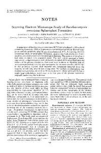
Fig. 1 — Difference between acquisition with SE (left) and BSE detector (right): The SE detector is strongly influenced by sample topography. The BSE is most strongly influenced by local specimen composition.
2.1
3
Calibration Procedure
Our calibration procedure for the SEM follows the methodology developed at the University of South Carolina [29]. It is a two-step process:
Operating Conditions
SEM operational parameters such as the detector type, accelerating voltage, working distance, etc. will affect the quality of the images. In this regard, the major requirements for image correlation in an SEM are (a) adequate image contrast, (b) random texture in the images, (c) appropriate spatial frequency in the random texture (d) temporal invariance in the images and (e) minimal image changes during the rigid-body motion of the specimen. Since SE detector imaging (which depends on topography of the sample) will violate (e) in most cases, BSE imaging is preferred. Moreover, the surface texture is improved when using the BSE detector (see Fig. 1). Since BSE imaging is also slightly affected by topography, in this work we chose to acquire all BSE images at a low accelerating voltage. In this way, the primary beam electrons do not penetrate deeply into the specimen. Another advantage of a low voltage incident beam is that surface details are enhanced in comparison to high voltage [27].
2.2
Figure 2 shows a schematic of two common models for the SEM imaging process. At low magnification (lesser than 1000×), the general model of perspective (or central) projection is applied because the observed area and electron beam sweep angle are both large. At higher magnification, the electron beam scanning angle is small and projection rays can be considered as parallel: the center of projection is at infinity and the parallel projection typically is assumed. In addition to these projection issues, the SEM imaging process is obviously not distortion free. These distortions must be taken into account and as we will see in Section 5.1, classic parametric models (radial and tangential distortion effects) are clearly not sufficient. The calibration procedure we use is explained in Section 3.
Parallel and Perspective Projections
1. Determination of the distortion removal function (warping function) based on a series of in-plane translations of a flat, randomly textured, calibration target. This warping function transforms the SEM imaging system into an ideal, distortion-free, virtual imaging sensor. 2. Calibration of this virtual imaging sensor through a traditional bundle-adjustment calibration technique. This step requires another image sequence of the same target undergoing arbitrary rigid-body motions. As will be shown below, the first step in the calibration process uses digital image correlation to precisely measure the displacements1 into the image sequence undergone by a set of arbitrary chosen points: the so-called “image matching” or “image registration” problem. This novel approach greatly simplifies the second step in the process by completely eliminating the need for a calibration target made up of fiducial markers such as ellipses or crossing lines. This is particularly important since, for obvious reasons, it is rather difficult, if not impossible, to realize a proper dedicated target which is suitable at high magnifications.
3.1
SEM Imaging Sensor
A priori Distortion Removal z B
90◦
100µm −x A
y
100µm
Rays ≈ parallel
C
Fig. 3 — Motions of the calibration target made with the translation stage for the estimation of the distortion removal functions. The given numerical values are suitable for magnification 200×.
Specimen
The determination of the warping function which transforms the physical imaging sensor into an ideal, virtual sensor 1A
Fig. 2 — At low magnification, perspective projection is used. At high magnification, parallel projection is typically employed.
displacement of a given object point into the imaging space is often called a “disparity”. A set of disparities related to the same two images is commonly referred as a “disparity map”.
plane is accomplished by acquiring a series of images of a randomly textured planar target undergoing in-plane translations [30, 29]. The theoretical background of this technique comes from the theoretical fact that any perspective transformation (and so any affine transformation) transforms a line into a line [5]. While only two known, non-parallel translations are required to determine the a priori distortion removal function, the accuracy of the warping functions can be greatly improved using additional (unknown) translations. A typical translation sequence is illustrated in Fig. 3 (AB and AC are usually chosen as the two know motions). As noted previously, the disparity maps for each image of the translation sequence with respect to a common reference image are computed using digital image correlation. To establish the warping function, software has been developed [14] to accurately determine the two B-spline vector functions relating image coordinates to coordinates on a virtual sensor plane; here, the calibration object is the virtual sensor plane.
3.2
Calibration
After determining the warping function that establish the ideal, virtual sensor plane, the virtual imaging system can be calibrated using bundle adjustment techniques. The bundle adjustment technique was originally developed for photogrammetry applications [3, 16, 17], i.e., the shape measurement using multiple views of an object. The technique has since been used with great success for various single camera calibration applications [4, 19]. It is clear that a reliable shape measurement using different views of a rigid object can only be made if sufficiently large triangulation angles are realized between the different orientations of the imaging system. Equivalently, sufficient triangulation angles can be realized using a stationary imaging system by rotating the calibration object in front of it. This principle is used to achieve reliable calibration of the virtual imaging system by moving the calibration target with the SEM rotation stage.
4
Automated 3-D Reconstruction Calibration Parameters
Image 1
Image 2
Feature Point Detection
Feature Point Detection
Epipolar Geometry Estimation
Motion Estimation
Feature Point Detection
Point Set Matching
Point Set Matching
Dense Matching
Image n
Dense Matching
Epipolar Geometry Estimation
Motion Estimation
Triangulation
3-D Shape
Fig. 4 — Steps of the Automated 3-D Reconstruction
M
m3
m1
C1
m2
C2 T2→1
C3 T2→3
Fig. 5 — Measuring the 3-D shape of a moving specimen is equivalent to measuring the shape of a static specimen with a moving imaging sensor.
The most common approach for calibration and use of a single-sensor imaging system in 3-D surface reconstruction is to require accurate knowledge of the rigid-body object motions within a sequence of images (see Fig. 4). To mitigate the requirement for accurate motions, a novel approach is proposed that does not require any information regarding the required rigid-body motions. Indeed, a relationship exists between any image pair in the scene: the epipolar geometry [5, 23]. This geometry depends upon the relative positions of the two imaging sensor locations. If this geometry can be estimated from a pair of images in the sequence, then the rigid-body transformation between the two respective views can be estimated. By repeating this process for each image pair, the motion between each view and then the general motion of the scene is obtained. The main problem in implementing this approach is the estimation of the epipolar geometry from a pair of images. This is a rather delicate process and will not be fully developed here; the reader can refer to [1, 35, 37] for details. The first stage in this process is the extraction of some points (called feature points) from each image in order to obtain appropriate corresponding matches throughout the image sequence.
Feature Points Extraction Point detectors are most often compared with respect to their localization accuracy criterion. For this work, where the precise location of a feature point in the image (e.g., a corner) is not required but the ability to repeatedly identify corresponding points in the detection process is paramount, the work of Schmid et al. [28] indicates that the best detector evaluated with this criterion is the Harris detector [9].
Feature Points Matching In order to estimate the epipolar geometry between each pair of images, feature points are optimally matched using a Zero mean Normalized Cross Correlation (ZNCC) function. To prevent false matching, a robust method (Least Median of Squares) is used to detect and remove outliers.
Epipolar Geometry and Motion Estimation A minimum of seven point correspondences is required to estimate the epipolar geometry with an appropriate parameterization. In practice, an 8-point algorithm [20] is implemented which uses eight or more point pairs. To improve the stability of the process, isotropic scaling is applied to the coordinates [10] before carrying out the 8-point algorithm. Finally, an
optimization approach is used to minimize a physically meaningful quantity such as the distance from each point to the appropriate epipolar line. Then, using the intrinsic parameters given by the calibration, the motion is recovered [13, 38] (note that specific scene information is required to recover the scale factor for the magnitude of the translation).
Dense Matching and Refinement of the Estimated Motion After the epipolar geometry is estimated, one approach to complete the matching process for each feature point restricts the search area to its epipolar line and the surrounding area, oftentimes referred to as the “epipolar band” (thick epipolar line). In this work, a different approach is employed. Using the feature points where corresponding matching points have been identified, an estimation of the disparity map is determined in order to make the dense correlation easier: a triangular mesh is generated [8] from the matched points and then the disparity map is estimated for each point by interpolation into the triangle which contains it. Once the dense disparity map is computed, the epipolar geometry is improved as well as the corresponding motion.
• • • • • •
200× magnification non-dimensional spot-size of seven 10mm working distance accelerating voltage of 8kV seven-bit gray scale for all images (1024 × 884 size) 1.3mm by 1.1mm field of view
Figure 6 shows three fields of view for a US penny. The 200× coin detail shows a speckle texture that is adequate for selective use of digital image correlation to identify and match corresponding subsets during rigid-body motion. Note that the 200× image has a small depth range (< 50µm) does not introduce significant perspective distortion to the disparity maps between the images in a translation sequence. Thus, the randomly textured regions of the coin can be considered “flat” and be used for the computation of the a priori distortion removal function.
5.1
Calibration
translation sequence
reference
(29 images)
image
Triangulation As shown in Fig. 5, triangulation is used to compute the 3-D coordinates of a point that is common to at least two images. The 3-D information for each point is recovered by intersecting the different rays defined by the optical center of the sensor and the projected point in the image. Since the rays may not intersect, an over determined equation system is solved using a bundle-adjustment process to minimize the distance between the 2-D image point and the reprojection of the computed 3-D point. Since the translation component of the rigid-body motion linking two views is estimated up to an unknown scale factor, the 3-D shape is also reconstructed up to the same scale factor. The scale factor can be determined (a) knowing a distance between two points on the specimen and/or (b) knowing the magnitude of one translation component of the rigid-body motion of a given view in the image sequence.
5
Experiment and Results
1×
50×
image correlation (subset size 35) arbitrary motion sequence
(24 images)
Fig. 7 — Overview of calibration procedure: this first image of the translation sequence is correlated with the all other images of both the sequences.
200× Closer view Fig. 8 — BSE detector images of the planar aluminum calibration target covered with a thin speckle pattern layer of gold realized by microlithography.
aluminum wafer
micro-scale speckle pattern (gold deposit)
specimen to measure (US penny coin)
200×
Fig. 6 — Specimen used for the experiment: a coin detail imaged with the BSE detector at magnification 200×.
For all experiments, a FEI ESEM Quanta 200 is operated in high-vacuum mode (SEM mode). The operational parameters for these studies are as follows: • BSE detector
carbon adhesive disc to maintain a (missing) second specimen
carbon paint to insure specimen/ wafer conductivity
Fig. 9 — Setup of the experiment: the coin to measure is stuck using a thin adhesive on an aluminum wafer covered with a gold speckle pattern deposited by microlithography.
2 1 0 -1 -2
x-distortion [pixel] 3 2 1 0 -1 -2 -3
0.01 3.47e-18 -0.01 -0.02
x-distortion [pixel] 0.1 0.05 0 -0.05 -0.1
0
200
400 600 x [pixel]
800
1000
0 100 200 300 400 500 y [pixel] 600 700 800
0
0 -1 -2
y-distortion [pixel]
200
400 600 x [pixel]
800
1000
0.04 0.03 0.02 0.01 0 -0.01
y-distortion [pixel]
1 0.5 0 -0.5 -1 -1.5 -2 -2.5 -3
0 100 200 300 400 500 y [pixel] 600 700 800
0.1 0.05 0 -0.05 -0.1
0
200
400 600 x [pixel]
800
1000
0 100 200 300 400 500 y [pixel] 600 700 800
0
200
400 600 x [pixel]
800
1000
0 100 200 300 400 500 y [pixel] 600 700 800
Fig. 10 — Distortion field computed by using the especially designed planar speckle pattern: up) along the image x-axis and bottom) along the image y-axis.
Fig. 11 — High-frequencies of the distortion field computed by using the especially designed planar speckle pattern: up) along the image x-axis and bottom) along the image y-axis.
Procedure
the specimen plane in the reference image) of 43 nanometers (error is less than 0.05 pixel in image space).
As shown in Fig. 7, the FEI ESEM is calibrated (a) using the a priori distortion removal technique based on a 29 image sequence of a translated target and (b) using bundle adjustment calibration of the perspective model based on a 24 image sequence of the same target undergoing arbitrary rigid-body motions. Since the a priori distortion removal technique requires that a planar calibration target contains an appropriate speckle pattern texture, an aluminum plate covered with a gold speckle pattern realized by a microlithography process (see Figs. 8 and 9) is employed for one set of experiments. Another set of experiments used the random texture on the US penny. Note that the relative ”flatness” of the coin detail should not produce significant heterogeneities in the disparity maps when the target is slightly translated at magnification 200×.
Results Using the Micro-lithography Target Figure 10 shows the distortion field of the SEM imaging system when using the target shown in Fig. 8. The magnitude of the distortion is up to 4 pixels in the corners of the images (size 1024 × 884). Careful inspection of the data in Fig. 10 indicates that the distortion field contains high-frequency distortion components. To investigate these features, a high-pass filter is applied to the distortion field shown in Fig. 10. Fig. 11 displays the two-dimensional form for the high frequency components. The data in Fig. 11 clearly shows a periodic structure in the distortion along the x- and y-axis of the images, with an amplitude of up to 0.1 pixel. This high-frequency distortion field is probably related to the scan control system for the electron beam. After performing the calibration process using bundleadjustment, the rotation sequence gives a standard deviation for the reprojection errors in the virtual sensor plane (which is
Results Using Coin Texture Figure 12 shows the distortion field of the SEM imaging system when using the random texture on the coin as the target for the a priori distortion removal technique. The results are very similar to those obtained by using the “ideal” planar target. The high frequency components are shown in Fig. 13. These components are slightly disturbed compared to those computed with the planar target sequence. After performing the calibration process by bundleadjustment, the rotation sequence gives a standard deviation of the re-projection errors in the virtual sensor plane 91 nanometers, which represents an error of less than 0.1 pixel in image space. Note that these values also include the correlation errors which are higher with the coin texture than the “ideal” speckle pattern used in the previous section. Interestingly, the bundle adjustment technique re-estimates the shape of the calibration target (the coin) while also computing the perspective model parameters of the imaging system. Due to the a priori distortion removal technique constraint, the target is first assumed to be perfectly flat. Assuming a flat object as the initial guess for the calibration by bundle-adjustment, Fig. 14 shows that the shape of the target is properly re-estimated.
5.2
3-D Reconstruction
The process described in Section 4 is used to complete the calibration and 3-D reconstruction process for a specific example. For this application, four images of the US penny were acquired at 200× (see Fig. 6). The four images were obtained after undergoing unknown rigid-body motions.
2 1 0 -1 -2
x-distortion [pixel] 3 2 1 0 -1 -2 -3
0.03 0.02 0.01 3.47e-18 -0.01 -0.02 -0.03 -0.04
x-distortion [pixel] 0.1 0.05 0 -0.05 -0.1
0
200
400 600 x [pixel]
800
1000
0 100 200 300 400 500 y [pixel] 600 700 800 0 -1 -2
y-distortion [pixel] 1 0.5 0 -0.5 -1 -1.5 -2 -2.5 -3
0
200
400 600 x [pixel]
800
1000
0 100 200 300 400 500 y [pixel] 600 700 800 0.05 0.04 0.03 0.02 0.01 3.47e-18 -0.01 -0.02
y-distortion [pixel] 0.1 0.05 0 -0.05 -0.1
0
200
400 600 x [pixel]
800
1000
0 100 200 300 400 500 y [pixel] 600 700 800
Fig. 12 — Distortion field computed by using the coin in replacement to the especially designed speckle pattern: up) along the image x-axis and bottom) along the image y-axis.
Since the US penny texture is used to obtain feature points and perform image correlation in this application, then the distortions shown in Figs. 12 and 13 will be similar to those present in these images. Hence, the distortion results for this application are not reported.
0
200
400 600 x [pixel]
800
1000
0 100 200 300 400 500 y [pixel] 600 700 800
Fig. 13 — High-frequencies of the distortion field computed by using the coin in replacement to the especially designed speckle pattern: up) along the image x-axis and bottom) along the image y-axis.
z [micron] 40 30 20 10 0
Feature Point Extraction A set of feature points is first extracted using Harris detector. This set is then processed to keep only the best feature points in a given circular neighborhood (typically 5 pixel radius) with respect to their Harris “cornerness” function response. Using this approach, good feature points are regularly scattered throughout the image and the epipolar geometry to estimate in the next steps is likely to be better [38]. Depending upon the image being used between 9200 and 9800 points are extracted.
Robust Matching For each pair of images, feature points are matched using: • • • •
ZNCC criterion 15 × 15 pixels correlation window Correlation threshold of 70% Least Median of Squares method to detect and remove outliers (false matches) while estimating the epipolar geometry
An average of 3100 pairs of points are robustly matched from each set containing initially 9500 points (about 100 initial matches were removed as outliers).
-10
-600 -400 -200 x [micron]0
200 400
400600 0 200 y [micron] -400-200 -600 600
Fig. 14 — Re-estimated 3-D shape of the coin target used for the calibration by bundle-adjustment. The shape is made up of three distinct areas, which corresponds to the three areas of interest selected for being matched by correlation in the rotation sequence (we avoid to correlate areas of high curvature where the image correlation is likely to be less accurate.
points to their epipolar line is 0.26 pixel). An estimation of the motion is recovered and a first approximation of the 3-D shape is computed. Figure 15 shows the reconstructed shape based on 3100 matched feature points.
Dense Matching From the matched feature points obtained previously, an estimation of the dense disparity map is computed and used as an initial guess for an optimization approach (maximization of the ZNCC score with affine transformation of the correlation window). Then, the epipolar geometry is refined (mean distance of points to their epipolar line is now 5.10−3 pixel) improving the motion estimates.
Triangulation Motion Estimation As the feature points are only extracted with pixel accuracy, the computation of the epipolar geometry is a first estimation for the following stage (at this point, the mean distance of
Figure 16 shows the 3-D shape of the coin detail reconstructed by triangulation of the dense sub-pixel disparity map. The results in Figure 16 confirm that the calibration and 3-D reconstruction processes can be performed with arbitrary rigid-
Acknowledgment The authors wish to thank Dr. Oscar Dillon, former director of the CMS division at NSF, and Dr. Julius Dasch at NASA HQ for their support of this work through grants NSFCMS-0201345 and NASA NCC5-174. In addition, the support of Dr. Dana Dunkelberger, Director of the USC Microscopy Center, by providing unlimited access to the FEI ESEM for our baseline studies is gratefully acknowledged.
References Fig. 15 — Reconstructed 3-D shape based on the 3100 matched feature points.
[1] X. Armanque and J. Salvi. Overall view regarding fundamental matrix estimation. Image and Vision Computing, 21(2):205–220, 2003. [2] Horst A. Beyer. Accurate calibration of CCD cameras. In Conference on Computer Vision and Pattern Recognition, 1992. [3] D. C. Brown. The bundle adjustment — progress and prospects. Int. Archives Photogrammetry, 21(3), 1976. [4] M. Devy, V. Garric, and J.J. Orteu. Camera calibration from multiple views of a 2D object using a global non linear minimization method. In International Conference on Intelligent Robots and Systems, Grenoble (France), sep 1997.
Fig. 16 — Reconstructed 3-D shape after dense sub-pixel matching by image correlation (rendering of 26400 sub-sampled 3-D points).
[5] Olivier Faugeras. Three-Dimensional Computer Vision: A Geometric Viewpoint. MIT Press, 1993. ISBN 0-26206158-9.
body motions using a single sensor imaging system such as the FEI ESEM.
[6] K. Galanulis and A. Hofmann. Determination of forming limit diagrams using an optical measurement system. In 7th International Conference on Sheet Metal, pages 245– 252, Erlangen (Germany), sep 1999.
6
Conclusion
Using a priori distortion removal methods, a FEI ESEM system has been calibrated and used to accurately measure the 3-D shape of an object. The experimental results from the calibration studies show the necessity for taking into account and correcting for distortions in the SEM imaging process. Moreover, the presence of high-frequencies components in the distortion field demonstrates that classic parametric distortion models are not sufficient in the case of an SEM. Furthermore, the results from preliminary 3-D shape measurements are promising; calibration accuracy is estimated to be ±0.05 pixel, which corresponded to ±43 nanometers for the objects being studied in this work.
7
Future Work
Work is on-going to utilize the a priori distortion removal process and extend the work to the accurate measurement of strains in SEM systems. Issues such as temporal stability, presence of an unknown scale factor in the 3-D reconstruction process and accuracy of the measurements will be primary areas of emphasis.
[7] D. Garcia, J.-J. Orteu, and M. Devy. Accurate calibration of a stereovision sensor: Comparison of different approaches. In 5th Workshop on Vision, Modeling, and Visualization, pages 25–32, Saarbrcken (Germany), nov 2000. [8] L. Guibas and J. Stolfi. Primitives for the manipulation of general subdivisions and the computation of voronoi diagrams. ACM Transaction On Graphics, 4(2):74–123, 1985. [9] C. Harris and M. Stephens. A combined corner and edge detector. In Alvey Vision Conference, pages 147–151, 1988. [10] Richard Hartley. In defence of the 8-point algorithm. In Fifth International Conference on Computer Vision (ICCV’95), pages 1064–1070, Boston (MA, USA), June 1995. [11] J. D. Helm, S. R. McNeill, and M. A. Sutton. Improved 3-d image correlation for surface displacement measurement. Optical Engineering, 35(7):1911–1920, 1996. [12] M. Hemmleb and M. Schubert. Digital microphotogrammetry - determination of the topography of microstructures by scanning electron microscope. In Second TurkishGerman Joint Geodetic Days, pages 745–752, Berlin (Germany), may 1997.
[13] T. Huang and A. Netravali. Motion and structure from feature correspondences: a review. In Proc. of IEEE, volume 82, pages 252–258, 1994.
[28] C. Schmid, R. Mohr, and C. Bauckhage. Evaluation of interest point detectors. International Journal of Computer Vision, 37(2):151–172, 2000.
[14] Correlated Solutions Inc. and Dorian Garcia. Vic2D and Vic3D softwares. http://www.correlatedsolutions.com, 2002.
[29] H. Schreier, D. Garcia, and M. A. Sutton. Advances in light microscope stereo vision. Experimental Mechanics, 2003. Submitted.
[15] Z. L. Khan-Jetter and T. C. Chu. Three-dimensional displacement measurements using digital image correlation and photogrammic analysis. Experimental Mechanics, 30(1):10–16, 1990.
[30] Hubert W. Schreier. Calibrated sensor and method for calibrating same. Patent Pending, nov 2002.
[16] Karl Kraus. Photogrammetry, volume 1: Fundamentals and Standard Processes. Dmmler/Bonn, 1997. ISBN 3427-78684-6. [17] Karl Kraus. Photogrammetry, volume 2: Advanced Methods and Applications. Dmmler/Bonn, 1997. ISBN 3-42778694-3. [18] A.J. Lacey, S. Thacker, S. Crossley, and R.B. Yates. A multi-stage approach to the dense estimation of disparity from stereo sem images. Image and Vision Computing, 16:373–383, 1998. [19] J.-M. Lavest, M. Viala, and M. Dhome. Do we really need an accurate calibration pattern to achieve a reliable camera calibration? In 5th European Conference on Computer Vision, pages 158–174, Freiburg (Germany), 1998. [20] H.C. Longuet-Higgins. A computer algorithm for reconstructing a scene from two projections. Nature, 293:133– 135, September 1981. [21] P. F. Luo, Y. J. Chao, and M. A. Sutton. Application of stereo vision to 3-D deformation analysis in fracture mechanics. Optical Engineering, 33:981, 1994. [22] P. F. Luo, Y. J. Chao, M. A. Sutton, and W. H. Peters. Accurate measurement of three-dimensional deformable and rigid bodies using computer vision. Experimental Mechanics, 33(2):123–132, 1993. [23] Q.-T. Luong and O. D. Faugeras. The fundamental matrix : Theory, algorithms and stability analysis. The International Journal of Computer Vision, 1(17):43–76, 1996. [24] E. Mazza, G. Danuser, and J. Dual. Light optical measurements in microbars with nanometer resolution. Microsystem Technologies, 2:83–91, 1996. [25] H. L. Mitchell, H. T. Kniest, and O. Won-Jin. Digital photogrammetry and microscope photographs. Photogrammetric Record, 16(94):695–704, 1999. [26] J.-J. Orteu, V. Garric, and M. Devy. Camera calibration for 3-D reconstruction: Application to the measure of 3-D deformations on sheet metal parts. In European Symposium on Lasers, Optics and Vision in Manufacturing, Munich (Germany), jun 1997. [27] R.G. Richards, M. Wieland, and M. Textor. Advantages of stereo imaging of metallic surfaces with low voltage backscattered electrons in a field emission scanning electron microscope. Journal of Microscopy, 199:115–123, August 2000.
[31] M. A. Sutton, T. L. Chae, J. L. Turner, and H. A. Bruck. Development of a computer vision methodology for the analysis of surface deformations in magnified images. In George F. vander Voort, editor, MiCon 90: Advances in Video Technology for Microstructural Control, ASTM STP 1094, pages 109–132, Philadelphia (USA), 1990. American Society for Testing and Materials. [32] M. A. Sutton, S. R. McNeill, J. D. Helm, and H. W. Schreier. Computer vision applied to shape and deformation measurement. In Elsevier Science, editor, International Conference on Trends in Optical Nondestructive Testing and Inspection, pages 571–589, Lugano (Switzerland), 2000. [33] M. A. Sutton, W. J. Wolters, W. H. Peters, W. F. Ranson, and S. R McNeill. Determination of displacements using an improved digital correlation method. Image and Vision Computing, 21:133–139, 1983. [34] P. Synnergren and M. Sj odahl. A stereoscopic digital speckle photography system for 3-D displacement field measurements. Optics and Lasers in Engineering, 31:425–443, 1999. [35] P. Torr. and D. Murray. The development and comparison of robust methods for estimating the fundamental matrix. International Journal of Computer Vision, 24(3):271–300, 1997. [36] F. Vignon, G. Le Besnerais, D. Boivin, J.-L. Pouchou, and L. Quan. 3D reconstruction from scanning electron microscopy using stereovision and self-calibration. In Physics in Signal and Image Processing, Marseille (France), January 2001. [37] Zhengyou Zhang. Determining the epipolar geometry and its uncertainty: A review. Technical Report 2927, INRIA, July 1996. [38] Zhengyou Zhang. A new multistage approach to motion and structure estimation: From essential parameters to euclidean motion via fundamental matrix. Technical Report 2910, INRIA, June 1996.