diagnostics Article
Automated Micro-Object Detection for Mobile Diagnostics Using Lens-Free Imaging Technology Mohendra Roy 1,2 , Dongmin Seo 1 , Sangwoo Oh 1,3 , Yeonghun Chae 4 , Myung-Hyun Nam 5 and Sungkyu Seo 1, * 1 2 3 4 5
*
Department of Electronics and Information Engineering, Korea University, Sejong 30019, Korea;
[email protected] (M.R.);
[email protected] (D.S.);
[email protected] (S.O.) Department of Physics, Rajiv Gandhi University, Arunachal Pradesh, Doimukh 791112, India Maritime Safety Research Division, Korea Research Institute of Ships and Ocean Engineering, Daejeon 34103, Korea Department of Big Data Science, University of Science and Technology, Daejeon 305350, Korea;
[email protected] Department of Laboratory Medicine, Korea University Ansan Hospital, Ansan 15355, Korea;
[email protected] Correspondence:
[email protected]; Tel.: +82-44-860-1427
Academic Editor: Aydogan Ozcan Received: 29 December 2015; Accepted: 27 April 2016; Published: 5 May 2016
Abstract: Lens-free imaging technology has been extensively used recently for microparticle and biological cell analysis because of its high throughput, low cost, and simple and compact arrangement. However, this technology still lacks a dedicated and automated detection system. In this paper, we describe a custom-developed automated micro-object detection method for a lens-free imaging system. In our previous work (Roy et al.), we developed a lens-free imaging system using low-cost components. This system was used to generate and capture the diffraction patterns of micro-objects and a global threshold was used to locate the diffraction patterns. In this work we used the same setup to develop an improved automated detection and analysis algorithm based on adaptive threshold and clustering of signals. For this purpose images from the lens-free system were then used to understand the features and characteristics of the diffraction patterns of several types of samples. On the basis of this information, we custom-developed an automated algorithm for the lens-free imaging system. Next, all the lens-free images were processed using this custom-developed automated algorithm. The performance of this approach was evaluated by comparing the counting results with standard optical microscope results. We evaluated the counting results for polystyrene microbeads, red blood cells, HepG2, HeLa, and MCF7 cells lines. The comparison shows good agreement between the systems, with a correlation coefficient of 0.91 and linearity slope of 0.877. We also evaluated the automated size profiles of the microparticle samples. This Wi-Fi-enabled lens-free imaging system, along with the dedicated software, possesses great potential for telemedicine applications in resource-limited settings. Keywords: lens-free; algorithm; telemedicine; cytometer; RBC
1. Introduction Analysis of micro-objects, e.g., cells and micro-particles, is among the major tasks in pathology, biological research, and material science research. Concentrations and other physiological information regarding cells, such as their size and shape, are crucial information for a pathologist or a physician to reach a diagnostic conclusion. For example, information about the red blood cell (RBC) concentration, white blood cell concentration, and platelet concentration of a patient’s whole blood sample plays an important role in early diagnosis of many diseases. In most labs, especially in resource-limited Diagnostics 2016, 6, 17; doi:10.3390/diagnostics6020017
www.mdpi.com/journal/diagnostics
Diagnostics 2016, 6, 17
2 of 15
settings, this type of study is generally conducted using a conventional optical microscope and hemocytometer. In this conventional method, an expert manually inspects the samples, which is tedious and prone to subjective error. On the other hand, recent biomedical research frequently requires the analysis of increasingly large numbers of cell and particle samples [1]. Resource-rich laboratories often use sophisticated automated alternatives, such as a Coulter counter and flow cytometer, to handle large sample numbers [2]. However, these automated systems are bulky and expensive, which limits their application and makes them impractical for resource-limited settings. Furthermore, there is increasing demand for a compact, high-throughput, fast, and cost-effective point-of-care cytometry system that can be operated by a non-expert user. These are the major challenges that most of the biomedical labs are currently trying to address. Many research groups have made extensive progress in this direction. Current advances in micro- and nanotechnology have improved the utility of micro- and nanoscale devices and the possibility of overall device miniaturization. These miniature devices retain advantages such as low power consumption and the possibility of using batch processing to lower the unit cost. Kumar et al. recently demonstrated a simple, cost-effective way to detect sickle RBC disease [3]. Richards et al. used advanced microfabrication technology to demonstrate a novel micro-Coulter counter that can efficiently detect microparticles [4]. Stewart and Pyayt demonstrated a microscale flow cytometry system that uses advanced microfluidic technology to efficiently detect cells and their sizes [5]. All these methods are based on microfluidic technology and supported by an independent liquid flow source such as a peristaltic pump. However, these support systems are bulky and very challenging to miniaturize, which affects the overall size of the system. Many research groups successfully demonstrated other alternatives to detect and characterize microparticles. Among them, the imaging of microparticles and cells using a compact lens-free imaging system promises significant advantages [6]. Bishara et al. successfully demonstrated a compact lens-free holographic microscopy system with a spatial resolution of 0.6 µm [7]. Isikman et al. demonstrated a lens-free optical tomographic microscope with a large field of view [8]. Seo et al. demonstrated a lens-free holographic imaging system that can perform on-chip cytometry [9]. All these methods are based on an unconventional imaging technology called the lens-free imaging technology which is gaining in popularity because of its advantages such as high throughput, compact size, low cost, and reagent-free detection [10]. A lens-free imaging system is a simple arrangement of optoelectronic devices for capturing the diffraction patterns of micro-objects that are located very close to the optoelectronic sensor, e.g., a complementary metal–oxide–semiconductor (CMOS) or charge-coupled device (CCD) image sensor [11]. The characteristics of a diffraction pattern generated upon illumination of the sample plane with coherent light are governed by the physical and optical properties of the object, such as its size, shape, and refractive index [11,12]. These properties can be obtained by characterizing the captured diffraction pattern [12]. However, to date, these types of analysis have been done manually or using semi-automated software such as Image J, which requires manual assistance to provide the threshold range, circularity, and other parameters. Further, this type of software is generally designed for the analysis of optical micrographs. Therefore, there is a need for a fully automated, dedicated algorithm for fast, hassle-free characterization of the diffraction patterns in a lens-free image. In our previous work we tried to implement an automated method based on global threshold [13,14]. However, the algorithm shows a correlation in the range of 0.68 to 0.89 for microbeads. This is due to the variation in the background intensity within the same sample. We tried to address this issue by adopting a local threshold method. In this paper, we introduce an automated method that can automatically detect, obtain, and analyze the features of the diffraction patterns of micro-objects. The approach is based on the detection of the midpoint of a diffraction pattern, followed by identification of the diffraction parameters, such as the central maxima value (CMV), width of the central maxima (WCX), width of the central minima (WCN), and peak-to-peak distance (PPD) [13,14]. For this purpose, we develop a mechanism to locally obtain the signal pixels and a clustering procedure to acquire the central positions of the diffraction
Diagnostics 2016, 6, 17
3 of 15
patterns. The detected parameters are used for filtering as well as to obtain the physical properties of the micro-objects. The algorithm is optimized for fast, accurate performance by comparing the results with standard microscope results. Finally, the performance of this approach is investigated Diagnostics 2016, 6, 17 3 of for 12 various samples: microbeads, RBCs, and HeLa, MCF7, and HepG2 cells. The quantified results are compared positions of the diffraction patterns. The detected parameters are used for filtering as well as to with the results of a conventional standard method to evaluate the agreement between the two. obtain the physical properties of the micro-objects. The algorithm is optimized for fast, accurate performance by comparing the results with standard microscope results. Finally, the performance of 2. Material and Methods this approach is investigated for various samples: microbeads, RBCs, and HeLa, MCF7, and HepG2 cells. The quantified results are compared with the results of a conventional standard method to 2.1. Lens-Free Imaging evaluate the agreement between the two.
Cell 2.imaging is among the basic methods used in cytometry and feature profiling of micro-objects. Material and Methods However, a high-resolution microscope is not the only choice for this purpose. The necessary 2.1. Lens-Free Imaging for cell cytometry and particle analysis can be provided by alternative vital information required arrangementsCell such as a islens-free shadow imagingused system [6]. Theand lens-free imagingofsystem is imaging among the basic methods in cytometry feature profiling However, microscope is not the choice forcoherent this purpose. a compactmicro-objects. system consisting ofaahigh-resolution CCD or CMOS image sensor andonly a partially lightThe source, e.g., necessary vital information required for cell cytometry and particle analysis can be provided by a light-emitting diode (LED) [13–15]. A schematic of the custom-built lens-free imaging system alternative arrangements such as a lens-free shadow imaging system [6]. The lens-free imaging is shownsystem in Figure 1. The schematic illustrates the simplicity of the fabricated setup. In our is a compact system consisting of a CCD or CMOS image sensor and a partially coherent system, we used a five-megapixel (1920 ˆ 2560 monochrome CMOS image sensor (EO-5012M, light source, e.g., a light-emitting diode (LED)pixel) [13–15]. A schematic of the custom-built lens-free is shown NJ, in Figure 1. The the simplicity of the Edmundimaging Optics,system Barrington, USA) thatschematic can be illustrates purchased at 14 USD perfabricated chip forsetup. the order of 2 andsensor In(MT9P031, our system, Aptina, we used Phoenix, a five-megapixel (1920 with × 2560 pixel) monochrome CMOS 2400 chips AZ, USA), a sensing area of 23.52 mmimage unit pixel size (EO-5012M, Edmund Optics, Barrington, NJ, USA) that can be purchased at 14 USD per chip for the of 2.2 µm, and a blue LED with a peak wavelength of 470 ˘ 0.5 nm (HT-P318FCHU-ZZZZ, Harvatek, order of 2400 chips (MT9P031, Aptina, Phoenix, AZ, USA), with a sensing area of 23.52 mm2 and Hsinchu City, Taiwan; costing approximately 3 USD) as a light source. A pinhole 300 ˘ 5 µm in unit pixel size of 2.2 μm, and a blue LED with a peak wavelength of 470 ± 0.5 nm size was mounted (HT-P318FCHU-ZZZZ, on the top of the LED to achieve uniform illuminates Harvatek, Hsinchu City, semi-coherent Taiwan; costing illumination approximately that 3 USD) as a light samples A pinhole cell-counting 300 ± 5 μm in size was mounted on polymethylmethacrylate the top of the LED to achieve(C-Chip, uniform C10288, loaded insource. a transparent chamber made of semi-coherent that samples loaded in(Raspberry a transparentPi, cell-counting chamber Invitrogen, Waltham,illumination MA, USA). Ailluminates single-board computer Raspberry Pi foundation, made of polymethylmethacrylate (C-Chip, C10288, Invitrogen, Waltham, MA, USA). A single-board Caldecote, UK) costing approximately 40 USD was used to record the captured images and to transmit computer (Raspberry Pi, Raspberry Pi foundation, Caldecote, UK) costing approximately 40 USD them wirelessly smartphone or a PC, where they werethem auto-processed the custom-developed was usedtotoa record the captured images and to transmit wirelessly to ausing smartphone or a PC, they were auto-processed usingCo. theLtd, custom-developed software. An wireless Edimax (Edimax software.where An Edimax (Edimax Technology Xinbei, Taiwan) 2.4 GHz adapter costing Technology Co. Ltd, Xinbei, Taiwan) 2.4 GHz wireless adapter costing about 10 USD was to within about 10 USD was used to facilitate the Wi-Fi connection. All these components wereused packed facilitate the Wi-Fi connection. All these components were packed within 9.3 × 9.0 × 9.0 cm3. This 3 9.3 ˆ 9.0 ˆ 9.0 cm . This fabricated system was used to obtain whole-frame lens-free images that offer fabricated system was used to obtain whole-frame lens-free images that offer a field of view a field of approximately view approximately 25 of times of amicroscope. 100ˆ optical microscope. 25 times that a 100×that optical
Figure 1. Schematic and working principle of the lens-free imaging system. (a) Schematic of the proposed system illustrating its simplicity with potential wireless file transfer facility; (b) cartoon of working principle of the formation of the diffraction pattern of a micro-object; (c) external view of the fabricated setup.
Diagnostics 2016, 6, 17
4 of 15
2.2. Sample Preparation We used several types of cell lines and microbead samples for this study. The preparation methods of these samples are described below. 2.2.1. Polystyrene Microbeads We used polystyrene microbeads (Thermo Scientific, Waltham, MA, USA) to examine the performance of the algorithm for particle counting and size determination. We prepared four heterogeneous samples with a wide particle size range (5–30 µm) by mixing in different concentrations with de-ionized (DI) water. These samples were then examined under the lens-free system and a standard optical microscope using a C-Chip. 2.2.2. RBCs RBC samples were collected from Korea University Ansan Hospital under institutional review board approval in a tube treated with ethylenediaminetetraacetic acid. The samples were then diluted with Roswell Park Memorial Institute (RPMI-1640, Thermo Scientific) media and loaded in a C-Chip for analysis under the proposed lens-free system and a standard optical microscope. 2.2.3. HepG2 Cells HepG2 cell lines were derived from human liver tissue from the American Type Culture Collection (ATCC HB-8065, Manassas, VA, USA) and grown in a high-glucose growth medium (Dulbecco Modified Eagle Medium, DMEM) supplemented with 10% heat-inactivated fetal bovine serum, 0.1% gentamycin, and a 1% penicillin/streptomycin solution under 95% relative humidity and 5% CO2 at 37 ˝ C. The cells were then trypsinized and separated from the 24-well plate and incubated for 2–5 min at 37 ˝ C. The incubated cells were washed and diluted with DMEM solution and then loaded in a C-Chip for analysis under the lens-free system and optical microscope. 2.2.4. MCF7 Cells A human breast cancer cell line (MCF7) was obtained from the American Type Culture Collection (ATCC HTB-22, Manassas, VA, USA). The cells were maintained in a solution of DMEM containing 1% penicillin/streptomycin solution, 0.1% gentamycin, and 10% calf serum at 95% relative humidity and 5% CO2 at 37 ˝ C. These cells were then trypsinized to separate them from the well plate, followed by incubation for 2–5 min at 37 ˝ C. The cells were then washed with DMEM solution and loaded in a C-Chip for examination under the lens-free system and optical microscope. 2.2.5. HeLa Cells A human cervical cancer cell line (HeLa, ATCC CCL-2) was collected from the American Type Culture Collection (Manassas, VA, USA). The cells were then maintained in a solution of DMEM containing 1% penicillin/streptomycin solution, 0.1% gentamycin, and 10% calf serum at 95% relative humidity and 5% CO2 at 37 ˝ C. The cells were separated from the 24-well plate by applying a trypsin solution and incubated for 2–5 min at 37 ˝ C. After incubation, the cells were washed and diluted in a DMEM solution and loaded in C-Chip for examination under the lens-free system and optical microscope. 2.3. Algorithm The algorithm used in this study contains a number of steps. The following sections describe the processes involved in this method in detail.
Diagnostics 2016, 6, 17
5 of 12
Diagnostics 2016, 6, 17
5 of 15 The algorithm used in this study contains a number of steps. The following sections describe the processes involved in this method in detail.
2.3.1. Summary of the Algorithm 2.3.1. Summary of the Algorithm As the signals of the diffraction patterns in a whole-frame lens-free image are significantly affected Asofthe of the the diffraction patterns in a using whole-frame lens-free image are owing significantly by that thesignals background, signals can be filtered a threshold [16]. However, to the affected by that of the background, the signals can be filtered using a threshold [16]. However, large field of view and non-uniform background, a global threshold is unsuitable for this purpose (see owing to the large field ofsegmentation view and non-uniform background, a global threshold is unsuitable the comparison of existing method ‘graythresh’ with our custom developed methodfor in this purpose (see the comparison of existing segmentation method ‘graythresh’ with our custom the Figures S1, S2 and Table S1 of the Supplementary Materials). Again, the strength of the signal and developed in themay Figures S2sample and Table S1 of the the value of themethod background vary S1, from to sample. To Supplementary understand this,Materials). we studiedAgain, lens-free strengthofofdifferent the signal and value the background vary from sample to sample. To This understand images samples (seeofFigure 2) and by may evaluating the 3D intensity profile. shows this, we studied lens-free images of different samples (see Figure 2) and by evaluating the 3D the variation in the background values and pixel values of the signals. In this context, it is necessary intensity profile. This shows the variation in the background values and pixel values of the signals. to acquire the signals locally [17]. We did this using a 10 ˆ 10 patch wise technique method [18]. In this context, it is necessary to acquire the signals locally [17]. We did this using a 10 × 10 patch To locate the midpoint of the filtered diffraction pattern, we employed a clustering method using wise technique method [18]. To locate the midpoint of the filtered diffraction pattern, we employed a a 25 ˆ 25 patch wise technique. The midpoints of the clusters were obtained by averaging the spatial clustering method using a 25 × 25 patch wise technique. The midpoints of the clusters were obtained coordinates of each of the filtered cluster elements in the 25 ˆ 25 window. Finally, we filtered the by averaging the spatial coordinates of each of the filtered cluster elements in the 25 × 25 window. unwanted diffraction noise by evaluating the circularity of the diffraction patterns. This algorithm is Finally, we filtered the unwanted diffraction noise by evaluating the circularity of the diffraction then implemented as application software as shown in the Figure 3. The following are the steps for the patterns. This algorithm is then implemented as application software as shown in the Figure 3. The realization of this algorithm. following are the steps for the realization of this algorithm.
Figure 2.2.Diffraction Diffractionpattern patternanalysis. analysis. Optical micrographs a single (a)µm 10 bead; μm bead; μm Figure Optical micrographs of aofsingle (a) 10 (b) 20(b) µm20 bead; bead; (c) RBC; (d) HeLa cell; (e) HepG2 cell; and (f) MCF7 cell; (g)–(l) diffraction images (c) RBC; (d) HeLa cell; (e) HepG2 cell; and (f) MCF7 cell; (g)–(l) diffraction images corresponding to corresponding to (a)–(f), (m)–(r) intensity profiles corresponding todifferences (g)–(l), with (a)–(f), respectively, (m)–(r) respectively, intensity profiles corresponding to (g)–(l), with statistical of statistical differences of 10 samples from each of these cell lines. 10 samples from each of these cell lines.
Diagnostics 2016, 6, 17 Diagnostics 2016, 6, 17
6 of 15 6 of 12
Figure ofof custom-developed Figure 3. 3. Snapshot Snapshotof ofthe thecustom-developed custom-developedapplication applicationsoftware. software.(a)(a)Snapshot Snapshot custom-developed Windows application software; (b) optical micrograph of region of interest at 100× magnification; (c) Windows application software; (b) snapshot of custom-developed Android application; (c) optical snapshot of custom-developed (d)(d) diffraction pattern of of a single microparticle; micrograph of region of interestAndroid at 100ˆ application; magnification; diffraction pattern a single microparticle; (e) intensity profile of the diffraction pattern in (d) explaining the custom-developed (e) intensity profile of the diffraction pattern in (d) explaining the custom-developeddiffraction diffraction parameters parameters along along the the dotted dotted red redline linein in(d). (d).
2.3.2. Study of Diffraction Images 2.3.2. Study of Diffraction Images We conducted a study to understand the features of the diffraction patterns of the micro-objects We conducted a study to understand the features of the diffraction patterns of the micro-objects that were captured by the fabricated lens-free imaging system. For this study, we selected six types that were captured by the fabricated lens-free imaging system. For this study, we selected six types of samples: 10 μm and 20 μm polystyrene beads, RBCs, and the HeLa, HepG2, and MCF7 cell lines. of samples: 10 µm and 20 µm polystyrene beads, RBCs, and the HeLa, HepG2, and MCF7 cell lines. We ensured the type and size of the sample by taking the optical micrograph of the same sample in We ensured the type and size of the sample by taking the optical micrograph of the same sample in 100× optical zoom. We evaluated the intensity profile for 10 different diffraction patterns of each 100ˆ optical zoom. We evaluated the intensity profile for 10 different diffraction patterns of each type of sample manually using Image J (NIH, Bethesda, MD, USA) [15]. The intensity profiles of all type of sample manually using Image J (NIH, Bethesda, MD, USA) [15]. The intensity profiles of all these samples are shown in Figure 2, which demonstrates that the diffraction patterns have almost these samples are shown in Figure 2, which demonstrates that the diffraction patterns have almost the the same features as the intensity profiles. However, the diffraction parameters for each type of same features as the intensity profiles. However, the diffraction parameters for each type of sample sample differ significantly. We identified these parameters as the CMV, WCX, WCN, and PPD [13], differ significantly. We identified these parameters as the CMV, WCX, WCN, and PPD [13], as shown as shown in Figure 3e. These parameters represent the physical optical properties of the in Figure 3e. These parameters represent the physical optical properties of the micro-objects [14]. micro-objects [14]. To detect and characterize these parameters, it is important to precisely locate the To detectofand these parameters, it is important to precisely locate position the position thecharacterize diffraction pattern. We also studied the 3D intensity profile (seethe Figure 4 of of the diffraction pattern. We also studied the 3D intensity profile (see Figure 4 of the samples to understand samples to understand the variation of the intensity profile within the sample as well as in between the samples. variation of the intensity profile within the sample as well as in between the samples. the
Diagnostics 2016, 6, 17 Diagnostics 2016, 6, 17
7 of 15
7 of 12
Figure intensityplot plotof oflens-free lens-free images (a)(a) 20 μm bead; (c) HepG2; (e) RBC; (g) Figure 4. 4. 3D3D intensity imagesofofsix sixsamples. samples. 20 µm bead; (c) HepG2; (e) RBC; MCF7; (i) HeLa cell; and (k) 10 μm bead. (b), (d), (f), (h), (j), and (l) are the 3D intensity plots (g) MCF7; (i) HeLa cell; and (k) 10 µm bead. (b), (d), (f), (h), (j), and (l) are the 3D intensity plots corresponding (e), (g), (i),and and(k), (k),respectively. respectively. corresponding to to (a),(a), (c),(c), (e), (g), (i),
2.3.3. Signal Acquisition 2.3.3. Signal Acquisition The signals of the diffraction patterns in a whole-frame image from a lens-free system were The signals of the diffraction patterns in a whole-frame image from a lens-free system were filtered using a 10 × 10 sliding window filter. A schematic representation of the windowing is shown filtered using a 10 ˆ 10 sliding window filter. A schematic representation of the windowing is shown in Figure 5b. The threshold value in a 10 × 10 window was calculated by finding the difference in Figure threshold value of inthe a 10 ˆ 10inwindow was calculated by finding the difference between5b. theThe maxima and minima pixels that window. If the pixel value difference between between the maxima and minima of the pixels in that window. If the pixel value difference the maxima and minima in that window exceeds 30 units, then the threshold value is equal between to half thethe maxima minima and in that window 30 units, then the threshold valueorisless equal tothe half sum ofand the maxima minima. Any exceeds pixel in that window having a value greater than thethreshold sum of the maxima and minima. Any pixel in thatimage window having value greater or less than value was recorded and stored in a binary of the same asize as the original image. theThe threshold value was recorded and stored in a binary image of the same size as the original image. window was kept moving until it reached the end of the image. The window was kept moving until it reached the end of the image.
Diagnostics 2016, 6, 17 Diagnostics 2016, 6, 17
8 of 15 8 of 12
Figure 5. Schematic workflow of of the the algorithm. algorithm. (a) fabricated Figure 5. Schematic of of the the workflow (a) Whole-frame Whole-frame image image from from the the fabricated lens-free imaging system; (b) schematic representation (not the actual representation of 10 × 10 lens-free imaging system; (b) schematic representation (not the actual representation of 10 ˆ 10 window) window) of the windowing method; (c) filtered binary image of (b); (d) detected and marked of the windowing method; (c) filtered binary image of (b); (d) detected and marked diffraction patterns diffraction patterns in a whole-frame lens-free image. in a whole-frame lens-free image.
2.3.4. 2.3.4. Clustering Clustering The pixels with their actual actual spatial spatial The filtered filtered binary binary image image contains contains only only the the probable probable signal signal pixels with their coordinates. Figure 5c shows a filtered binary version of a lens-free image. However, these coordinates. Figure 5c shows a filtered binary version of a lens-free image. However, these binary binary images images are are sparse sparse in in nature. nature. The The pixels pixels in in aa filtered filtered binary binary image image are are not not continuous, continuous, and and edge edge pixels pixels from two neighboring diffraction patterns are very difficult to assign to a particular origin (see from two neighboring diffraction patterns are very difficult to assign to a particular origin (see the the region interest in in Figure Figure 5c). 5c). The image also also contains contains some some unwanted unwanted noise noise pixels. pixels. To eliminate region of of interest The image To eliminate these 2525 patch-wise technique was used to these shortcomings, shortcomings, aa clustering clusteringmethod methodwas wasemployed. employed.AA2525× ˆ patch-wise technique was used find the spatial distance between the signal pixels. The pixels inside a particular window were to find the spatial distance between the signal pixels. The pixels inside a particular window were grouped basis of of the the calculated calculated spatial spatial distance. distance. Any spatial distance distance grouped together together on on the the basis Any pixel pixel having having aa spatial less less than than 33 pixel pixel units units from from the the neighboring neighboring pixels pixels was was considered considered as as aa probable probable cluster cluster member, member, and and any isolated pixels were neglected. The window was kept moving until it reached the any isolated pixels were neglected. The window was kept moving until it reached the end end of of the the image. averaging the image. The The tentative tentative midpoint midpoint of of aa cluster cluster or or diffraction diffraction pattern pattern was was calculated calculated by by averaging the spatial of each each cluster cluster element. element. spatial coordinates coordinates of 2.3.5. Diffraction Parameter Acquisition The CMV of a diffraction pattern is the pixel value of the midpoint. The CMVs of the diffraction patterns in ina awhole-frame whole-frame lens-free image obtained by mapping the calculated lens-free image werewere obtained by mapping the calculated midpointmidpoint positions positions from the binary clusters to image. the original image. WCX ofpattern a diffraction patternacross was from the binary clusters to the original The WCX of aThe diffraction was obtained obtained across the midpoint by calculating the number of all pixels in a row (or column), where the the midpoint by calculating the number of all pixels in a row (or column), where the pixel values were pixel values to the The WCN a diffraction pattern obtained across the similar to thewere CMV.similar The WCN of aCMV. diffraction patternofwas obtained across thewas midpoint by calculating midpoint byofcalculating the number of all pixels in athe row (or values column), where the pixel values were the number all pixels in a row (or column), where pixel were less than the CMV. less than the CMV.
Diagnostics 2016, 6, 17
9 of 15
2.3.6. Circularity Filter A study of the diffraction images of six different types of samples reveals that the diffraction patterns are circular. This property is an advantage for filtering unwanted diffraction patterns. Therefore, we implemented another filter, which evaluates the circularity of the diffraction patterns by calculating the aspect ratio of the WCX and the WCN. If the aspect ratio (WCX vertical/WCX horizontal) of a particular pattern is equal to 1, then it was considered; otherwise, it was neglected. Similarly, the circularity was obtained using the WCN. The filtered diffraction patterns were considered final and marked (Figure 5d). 2.3.7. Size Determination In this step, the PPDs of the filtered diffraction patterns were calculated. The PPD was evaluated by calculating the difference between the CMV and the minima of the diffraction pattern. The concentrations of the microparticles were calculated by evaluating the total number of filtered diffraction patterns. The sizes of the microparticles were obtained by converting the PPD to the original image as described in our previous work [14]. In this method, the original size of the objects from the detected PPD value were obtained using the equation Y “ 0.28X
(1)
where Y is the original size, and X is the PPD. A concise flowchart of all the steps of the algorithm is depicted in Figure 6.
Diagnostics 2016, 6, 17 Diagnostics 2016, 6, 17
1 of 12 10 of 15
Figure Figure 6. 6. Concise Concise flowchart flowchart of of the the algorithm. algorithm.
Diagnostics 2016, 6, 17
11 of 15
3. Results and Discussion As described in an earlier section, the features of the diffraction patterns of micro-objects were evaluated for six different types of samples. For this purpose, we used a 10 µm bead, a 20 µm bead, an RBC, and single HeLa, HepG2, and MCF7 cells. Optical micrographs and the corresponding lens-free images of each sample are shown in Figure 2. The intensity profiles were obtained manually by selecting an array of signal pixels from the diffraction patterns (see the red line in Figure 2g) using Image J (NIH, USA) image processing software. Thus, we obtained 10 different profiles of each type of sample for statistical study. The average coefficients of variation of the 10 µm bead, 20 µm bead, RBC, and HeLa, HepG2, and MCF7 cells are 0.53, 0.08, 0.06, 0.19, 0.23, and 0.21, respectively. The features of the diffraction patterns of all six samples are almost identical. However, each sample has different diffraction parameters. The statistical averages, i.e., the average of the diffraction parameters of 10 samples, for the 10 µm bead, 20 µm bead, RBC, and HeLa, HepG2 and MCF7 cells are as shown in the Table 1. This shows that the physical sizes of the diffraction patterns are almost the same, as there are very few differences in the WCX and WCN for all the sample types. However, the PPD and CMV differ significantly for each type of cell. Table 1. Statistical average of 10 samples for the diffraction parameters. Sample/Diffractin Parameters
10 µm Bead
20 µm Bead
RBC
HeLa
HepG2
MCF7
CMV WCX WCN PPD
144 8 4 38
132 7 4 86
176 11 5 69
149 6 4 65
151 7 5 89
139 7 4 85
We also studied the variation in the pixel values, particularly that of the background of the lens-free image, for each type of sample. We used the lens-free images of the 10 µm bead, 20 µm bead, RBC, HeLa, HepG2, and MCF7 cells. The 3D profiles of these images are shown in Figure 4. The study shows that the background of the lens-free image varies with the sample type. This is especially noticeable in the RBC sample (about 180) in Figure 4f, compared to other samples (approximately 160). This is due to the opacity, refractive index, and cell density of the samples. Again, in some samples (Figure 4f,l) the signal intensity is comparatively low (see magnified figures in the Supplementary Figure S3). To overcome all of these shortcomings, we need a mechanism to obtain the adaptive threshold. Therefore, we implemented the patch-wise technique method for this purpose. To determine the appropriate window size, we tested the algorithm with different window sizes and compared the results with the standard result. We also evaluated the processing time required for each window size. The results are shown in Figure 7a,b, respectively. The result indicates that the 10 ˆ 10 window, which provides more accurate results in less time, is ideal for obtaining the local threshold. This is also indicated by the size of the diffraction patterns. The total width (WCX + WCN) of the diffraction pattern for each sample is approximately 10–15 pixel units. Therefore, we implement the 10 ˆ 10 window in this algorithm. Again, the filtered binary images are sparse in nature (Figure 5c). To determine the midpoint of the diffraction patterns, we need to find the actual group of sparse signal pixels. For this purpose, we developed a clustering method in which the spatial distance between the signals is calculated. This was done by implementing a patch-wise technique to locally compute the spatial distances. We also optimized the size of this window for better performance in less processing time. The results are shown in Figure 7c,d. The results indicate that the 25 ˆ 25 window exhibits better performance with less processing time. We used these optimized parameters in the algorithm and implemented it on the custom-developed Android and Windows applications. Snapshots of the application layout are
Diagnostics 2016, 6, 17
12 of 15
shown in Figure 3a,b. Using this application software, we evaluated the counting and size profiling of Diagnostics 2016, 6, 17 2 of 12 the six types of samples.
Figure 7. Optimization of the windowing method. (a) Window size vs. counting result for obtaining Figure 7. Optimization of the windowing method. (a) Window size vs. counting result for obtaining the local threshold; (b) window size vs. processing time for obtaining the local threshold; (c) window the local threshold; (b) window size vs. processing time for obtaining the local threshold; (c) window size vs. counting result for clustering of filtered binary image; (d) window size vs. processing time for size vs. counting result for clustering of filtered binary image; (d) window size vs. processing time for clustering of filtered binary image. clustering of filtered binary image.
The Thecounting countingresults resultsfrom fromthe thecustom-developed custom-developedalgorithm algorithmfor forall allsix sixsamples sampleswere werecompared compared with the standard optical microscope results. Figure 8a compares the counting performance with the standard optical microscope results. Figure 8a compares the counting performanceof ofthe the two shows a correlation of 0.91. The The linearity of theofcounting resultsresults from twomodalities. modalities.The Thecomparison comparison shows a correlation of 0.91. linearity the counting the two modalities is compared in Figure 8b. This linearlinear behavior with awith slope of 0.877 and from the two modalities is compared in Figure 8b.shows This shows behavior a slope of 0.877 2 value 2 Rand of 0.820. In addition, the size profiling results from the automated method were compared R value of 0.820. In addition, the size profiling results from the automated method were with the results the standard optical microscope. The results for samples #1–4 are shown compared withfrom the results from the standard optical microscope. Thebead results for bead samples #1–4 inare Figure 8c–f, The correlation these comparisons are 0.947, 0.919, shown in respectively. Figure 8c–f, respectively. Thecoefficients correlationofcoefficients of these comparisons are0.906, 0.947, and 0.707, respectively, indicates that indicates the resultsthat of the agree with those of 0.919, 0.906, and 0.707,which respectively, which the proposed results of system the proposed system agree the conventional The average the size determination is about 1.6 µm Table S2 with those of themethod. conventional method.error The for average error for the size determination is (see about 1.6 μm in(see Supplementary). Table S2 in Supplementary).
Diagnostics 2016, 6, 17 Diagnostics 2016, 6, 17
13 of 15 3 of 12
Figure 8. Comparison Comparisonof ofautomatically automatically processed result with standard microscope results. processed result with standard microscope results. (a) (a) Comparison different samples; (b) linearity comparison of automatically the automatically processed Comparison for for six six different samples; (b) linearity comparison of the processed and and standard microscope results samples (a); (c)–(f)comparison comparisonofofauto-processed auto-processed size size results standard microscope results for for sixsix samples in in (a); (c)–(f) with the standard standard microscope microscope results results for for bead bead samples samples#1–4. #1–4.
4. Conclusions Conclusions
an automated automated micro-object micro-object counting method for a lens-free imaging system was In summary, an demonstrated. A comparison of the results obtained using this approach with those obtained using comparison standard method methodshows showsgood goodagreement agreementbetween betweenthe thetwo twomodalities. modalities. The correlation coefficient the standard The correlation coefficient of of 0.91 of show 0.877the show the agreement andbetween linearitythebetween theand automated and 0.91 and and slopeslope of 0.877 agreement and linearity automated conventional conventional Further, approaches. Further, aofcomparison of the size correlations results shows of 0.70 or approaches. a comparison the size results shows of correlations 0.70 or greater, which greater, which indicatesof the feasibilitysize of automated size characterization usingsystem. the lens-free system. indicates the feasibility automated characterization using the lens-free The lens-free The lens-free system is made ofcomponents, inexpensive e.g., components, e.g., an3LED 3 USD image and a CMOS system is made of inexpensive an LED costing USDcosting and a CMOS sensor image sensor costing 14 USD, the is cost of whichcompared is negligible compared to that of aauto-detection conventional costing 14 USD, the cost of which negligible to that of a conventional auto-detection system. The automated algorithm the result within 15 to 20 s. system. The automated algorithm processes theprocesses result within the range of the 15 range to 20 s.of Therefore, Therefore, this would be a cost-effective option for many research facilities. This type of system, this would be a cost-effective option for many research facilities. This type of system, along with the along with the dedicated algorithm, can evaluate several hundred diffraction patterns of dedicated algorithm, can evaluate several hundred diffraction patterns of micro-objects including RBCs micro-objects including RBCs cells and HeLa, HepG2, and MCF7 cells in a smart few minutes a moderate and HeLa, HepG2, and MCF7 in a few minutes using a moderate phone. using This combination smart phone. Thislens-free combination a automated Wi-Fi-enabled lens-free system andprovide automated detection of a Wi-Fi-enabled systemof and detection software would a cost-effective software would provide a cost-effective telemedicine facility for early diagnosis in resource-limited telemedicine facility for early diagnosis in resource-limited settings. However there is more scope to settings. However is morethe scope upgrade thesmall system to analyze the poor signals upgrade the systemthere to analyze poortosignals from microparticles (less than 2 µm).from Thissmall may microparticles than 2 μm). may be achieved by introducing sophisticated sensors be achieved by (less introducing more This sophisticated sensors with lower pixel more size alongside high density. withautomated lower pixel size alongside highalgorithm density. An automated recognition such as a An feature recognition such as a deepfeature learning algorithmalgorithm may be an added deep learning algorithm may be an added advantage for auto recognition of the type of cells. This advantage for auto recognition of the type of cells. This will eradicate the dependency of the current will eradicate thediffraction dependency of the current algorithm the diffraction parameters, which may be algorithm on the parameters, which may be aon scope for future research. a scope for future research. Supplementary Materials: The Supplementary files are available online at www.mdpi.com/2075-4418/6/2/17/s1. Supplementary Materials: The following are available online at www.xxx/xxx.
Acknowledgments: This research was supported by the Basic Science Research Program (Grant#:2013-010832, Grant#:2014R1A6A1030732) through the National Research Foundation of Korea (NRF) funded by the Ministry
Diagnostics 2016, 6, 17
14 of 15
Acknowledgments: This research was supported by the Basic Science Research Program (Grant#:2013-010832, Grant#:2014R1A6A1030732) through the National Research Foundation of Korea (NRF) funded by the Ministry of Science, ICT & Future Planning and the Ministry of Education. This work was also supported by the Korea Research Institute of Ships and Ocean Engineering (KRISO) Endowment-Grant (PES1870). Author Contributions: Mohendra Roy has contributed for the conception, design of the algorithm, data analysis and interpretation. He also wrote the draft of this manuscript. Dongmin Seo has contributed for the experimental set-up, data collection and handling of the biological cell lines. Sangwoo Oh has contributed for the experimental set-up and revision of this article. Yeonghun Chae has contributed for the experimental set-up and design of the algorithm. Myung-Hyun Nam has contributed for provision of the various cell lines and discussion as a clinical expert in the field of mobile diagnostics. Sungkyu Seo is the principal investigator and contributed for the conception, design of this work, and manuscript writing. He has also contributed for the revision and final approval of the manuscript to be published. Conflicts of Interest: The authors declare no conflict of interest.
References 1. 2. 3.
4. 5. 6.
7. 8.
9. 10. 11. 12. 13. 14.
15.
16.
Li, P.; Lin, B.; Gerstenmaier, J.; Cunningham, B. A new method for label-free imaging of biomolecular interactions. Sens. Actuator B Chem. 2004, 99, 6–13. [CrossRef] Purvi, N.; Giorgio, T. Cell size and surface area determined by flow cytometry. Ann. N. Y. Acad. Sci. 1994, 714, 306–308. [CrossRef] Kumar, A.; Patton, M.; Hennek, J.; Lee, S.; D’Alesio-Spina, G.; Yang, X.; Kanter, J.; Shevkoplyas, S.; Brugnara, C.; et al. Density-based separation in multiphase systems provides a simple method to identify sickle cell disease. Proc. Natl. Acad. Sci. USA 2014, 111, 14864–14869. [CrossRef] [PubMed] Richards, A.; Dickey, M.; Kennedy, A.; Buckner, G. Design and demonstration of a novel micro-Coulter counter utilizing liquid metal electrodes. J. Micromech. Microeng. 2012, 22, 115012. [CrossRef] Stewart, J.; Pyayt, A. Photonic crystal based microscale flow cytometry. Opt. Express 2014, 22, 12853–12860. [CrossRef] [PubMed] Greenbaum, A.; Luo, W.; Su, T.-W.; Göröcs, Z.; Xue, L.; Isikman, S.; Coskun, A.; Mudanyali, O.; Ozcan, A. Imaging without lenses: Achievements and remaining challenges of wide-field on-chip microscopy. Nat. Methods 2012, 9, 889–895. [CrossRef] [PubMed] Bishara, W.; Su, T.-W.; Coskun, A.; Ozcan, A. Lensfree on-chip microscopy over a wide field-of-view using pixel super-resolution. Opt. Express 2010, 18, 11181–11191. [CrossRef] [PubMed] Isikman, S.; Bishara, W.; Mavandadi, S.; Yu, F.; Feng, S.; Lau, R.; Ozcan, A. Lens-free optical tomographic microscope with a large imaging volume on a chip. Proc. Natl. Acad. Sci. USA 2011, 108, 7296–7301. [CrossRef] [PubMed] Seo, S.; Su, T.-W.; Tseng, D.; Erlinger, A.; Ozcan, A. Lensfree holographic imaging for on-chip cytometry and diagnostics. Lab Chip 2009, 9, 777–787. [CrossRef] [PubMed] Zhu, H.; Isikman, S.; Mudanyali, O.; Greenbaum, A.; Ozcan, A. Optical imaging techniques for point-of-care diagnostics. Lab Chip 2013, 13, 51–67. [CrossRef] [PubMed] Ozcan, A.; Demirci, U. Ultra wide-field lens-free monitoring of cells on-chip. Lab Chip 2008, 8, 98–106. [CrossRef] [PubMed] Kim, S.; Bae, H.; Koo, K.; Dokmeci, M.; Ozcan, A.; Khademhosseini, A. Lens-free imaging for biological applications. J. Lab. Autom. 2012, 17, 43–49. [CrossRef] [PubMed] Roy, M.; Jin, G.; Seo, D.; Nam, M.-H.; Seo, S. A simple and low-cost device performing blood cell counting based on lens-free shadow imaging technique. Sens. Actuators B Chem. 2014, 201, 321–328. [CrossRef] Roy, M.; Seo, D.; Oh, C.-H.; Nam, M.-H.; Kim, Y.; Seo, S. Low-cost telemedicine device performing cell and particle size measurement based on lens-free shadow imaging technology. Biosens. Bioelectron. 2015, 67, 715–723. [CrossRef] [PubMed] Jin, G.; Yoo, I.-H.; Pack, S.; Yang, J.-W.; Ha, U.-H.; Paek, S.-H.; Seo, S. Lens-free shadow image based high-throughput continuous cell monitoring technique. Biosens. Bioelectron. 2012, 38, 126–131. [CrossRef] [PubMed] Alyassin, M.; Moon, S.; Keles, H.; Manzur, F.; Lin, R.; Hæggstrom, E.; Kuritzkes, D.; Demirci, U. Rapid automated cell quantification on HIV microfluidic devices. Lab Chip 2009, 9, 3364–3369. [CrossRef] [PubMed]
Diagnostics 2016, 6, 17
17.
18.
15 of 15
Mondini, S.; Ferretti, A.; Puglisi, A.; Ponti, A. Pebbles and PebbleJuggler: Software for accurate, unbiased, and fast measurement and analysis of nanoparticle morphology from transmission electron microscopy (TEM) micrographs. Nanoscale 2012, 4, 5356–5372. [CrossRef] [PubMed] Gontard, L.; Ozkaya, D.; Dunin-Borkowski, R. A simple algorithm for measuring particle size distributions on an uneven background from TEM images. Ultramicroscopy 2011, 111, 101–106. [CrossRef] [PubMed] © 2016 by the authors; licensee MDPI, Basel, Switzerland. This article is an open access article distributed under the terms and conditions of the Creative Commons Attribution (CC-BY) license (http://creativecommons.org/licenses/by/4.0/).