FOR BROKEN BAR DETECTION AND DIAGNOSTICS

University of Rome “La Sapienza” Faculty of Engineering Department of Electrical Engineering

Ph.D. Thesis Chair of Electromechanical Constructions

HARMONIC CURRENT SIDEBAND INDICATORS (HCSBIs) FOR BROKEN BAR DETECTION AND DIAGNOSTICS IN CAGE INDUCTION MOTORS

Ph.D. Student Claudio Bruzzese

Supervising Professor

Co-Supervising Professor

Prof. Ezio Santini

Prof. Onorato Honorati

Academic Year 2006/2007

Dedico questa tesi di dottorato a molte persone. Innanzitutto la dedico a quanti vorranno leggerla con interesse, se ve ne saranno. La dedico a chi ha passione nella Scienza e nella Tecnica. A chi ama la Matematica e le simmetrie in Essa celate. La dedico a mio padre e mia madre, presenze costanti nella mia vita. Ai miei fratelli, Davide e Simone, distanti e vicini al tempo stesso. A tutti i miei maestri. Al prof. Ezio Santini, con gratitudine. Al prof. Onorato Honorati, con reverenza.

INDEX OF CONTENTS

INTRODUCTION (1): ABOUT THIS WORK

11

INTRODUCTION (2): STATE OF THE ART

14

REFERENCES OF THE INTRODUCTIONS (1), (2)

19

1

THE SQUIRREL CAGE INDUCTION MOTOR PHASE MODEL ACCORDING TO THE MUTUALLY-COUPLED LOOPS LINEAR THEORY AND TRANSFORMATION BY SYMMETRICAL COMPONENTS

1.1

INTRODUCTION: THE SYMMETRICAL THREE-PHASE CAGE INDUCTION MOTOR ELECTRICAL STRUCTURE

24 24

1.1.1 HYPOTHESES UNDERLYING THE MODEL 1.1.2 STATOR WINDINGS 1.1.3 ROTOR SQUIRREL CAGE

1.2

ELECTRIC AND MAGNETIC EQUATIONS OF THE (n, m+1) MODEL

28

1.2.1 INTRODUCTION 1.2.2 STATOR EQUATIONS 1.2.3 ROTOR EQUATIONS 1.2.4 END-RING EQUATION 1.2.5 COMPLETE MATRIX SYSTEM 1.2.6 PSEUDO-INDUCTANCE MATRIX AND ELECTRO-MAGNETIC TORQUE

1.3

THE (n,m+1) MODEL REDUCED FORM: THE (n,m) MODEL

37

1.4

THE SYMMETRICAL COMPONENTS TRANSFORMATION

39

1.4.1 INTRODUCTION 1.4.2 CURRENT TRANSFORMATIONS 1.4.3 VOLTAGE AND FLUX TRANSFORMATIONS 1.4.4 PSEUDO-INDUCTANCE MATRIX AND ELECTRO-MAGNETIC TORQUE TRANSFORMATIONS

3

1.5

TRANSFORMATIONS FOR CIRCULATING MATRICES

44

1.5.1 INTRODUCTION 1.5.2 TRANSFORMATION OF [RSS] 1.5.3 TRANSFORMATION OF [RRR] 1.5.4 TRANSFORMATION OF [LSS] 1.5.5 TRANSFORMATION OF [LRR]

1.6

TRANSFORMATION OF GENERIC ASYMMETRICAL MUTUAL INDUCTANCE RECTANGULAR MATRICES BY MEANS OF BI-SYMMETRICAL COMPONENTS

46

1.6.1 INTRODUCTION 1.6.2 MUTUAL INDUCTANCE MATRIX COMPLEX FORM 1.6.3 MUTUAL INDUCTANCE MATRIX TRANSFORMATION 1.6.4 UNILATERAL SERIES-FORM FOR TRANSFORMED MATRICES 1.6.5 MUTUAL PSEUDO-INDUCTANCE MATRIX TRANSFORMATION 1.6.6 ELECTRO-MAGNETIC TORQUE TRANSFORMATION 1.6.7 REDUCED FORM FOR THE TRANSFORMED ELECTROMAGNETIC TORQUE

1.7

TRANSFORMATION OF BI-SYMMETRICAL MUTUAL INDUCTANCE MATRICES (CYCLIC-SYMMETRIC MACHINES)

56

1.7.1 INTRODUCTION 1.7.2 BILATERAL TRANSFORMATION 1.7.3 UNILATERAL TRANSFORMATION 1.7.4 MUTUAL PSEUDO-INDUCTANCE MATRIX TRANSFORMATION 1.7.5 ELECTRO-MAGNETIC TORQUE TRANSFORMATION

1.A.

APPENDIX: FORTESQUE’S TRANSFORMATION FOR CIRCULATING MATRICES

64

1.A.1.

BASIC DEFINITIONS

64

1.A.2.

TRANSFORMATION OF A COMPLEX SQUARED (nxn) CIRCULANT MATRIX BY USING FORTESCUE’S MATRICES

65

PARTICULAR CASES OF FORTESCUE’S TRANSFORMATION FOR COMPLEX SQUARED CIRCULANT MATRICES

66

1.A.3.

1.A.3.1. MATRIX [A ] CIRCULANT AND REAL

4

1.A.3.2. MATRIX [A ] CIRCULANT AND SYMMETRIC-CONJUGATE 1.A.3.3. MATRIX [A ] CIRCULANT, REAL AND SYMMETRIC

1.B.

APPENDIX: BI-SYMMETRICAL COMPONENTS FOR RECTANGULAR (nxm ) MATRICES

70

1.B.1.

GENERIC ASYMMETRICAL MATRIX SYSTEM

70

1.B.2.

BASIC MATRIX SYMMETRICAL SYSTEM OF ORDER (p, q)

71

1.B.3.

MATRIX SYMMETRICAL COMPONENT SYSTEM OF ORDER (p, q)

72

1.B.4.

BI-SYMMETRICAL COMPONENTS DECOMPOSITION

73

1.B.5.

BI-SYMMETRICAL COMPONENTS-BASED TRANSFORMATION FOR A REAL MATRIX

76

1.C.

APPENDIX: MATH STATEMENTS (miscellaneous)

1.C.1.

DEFINITIONS FOR FOURIER SERIES

78 78

1.C.1.1. DEFINITION OF REAL UNILATERAL FOURIER SERIES 1.C.1.2. DEFINITION OF REAL BILATERAL FOURIER SERIES 1.C.1.3. DEFINITION OF COMPLEX BILATERAL FOURIER SERIES

1.C.2.

SOME PROPERTIES OF FORTESCUE’S TRANSFORMATION

80

1.C.2.1. BASIC PROPERTIES 1.C.2.2. DERIVED PROPERTIES

REFERENCES OF CHAPTER 1

2

FAULT-RELATED FREQUENCIES CALCULATION FOR A STEADY-STATE OPERATING MOTOR WITH BROKEN BARS

2.1

PHASE CURRENT FREQUENCIES PRODUCED BY A FAULTY CAGE

81

82 82

2.1.1 INTRODUCTION: PHYSICAL ASSESSMENT OF THE PHENOMENA 2.1.2 FAULT-RELATED FREQUENCIES CALCULATION

5

2.2

MULTI-PHASE SYMMETRICAL COMPONENTS FOR SINUSOIDAL TIME-VARYING CURRENT SYSTEMS

83

2.2.1 METHODOLOGY: FORTESCUE’S TRANSFORMATION 2.2.2 DECOMPOSITION OF A MULTI-PHASE ASYMMETRICAL SYSTEM OF CAGE CURRENTS

2.2.3 GRAPHICAL REPRESENTATION OF SYMMETRICAL SYSTEMS

2.3

SPACE HARMONICS OF AIR-GAP MAGNETIC FIELD PRODUCED BY PRACTICAL MULTI-PHASE WINDINGS FED BY GENERIC ASYMMETRIC ISO-FREQUENCY SINUSOIDAL TIME-VARYING CURRENT SYSTEMS

91

2.3.1 INTRODUCTION 2.3.2 HARMONIC DECOMPOSITION FOR AIR-GAP MAGNETIC FIELDS 2.3.3 MAGNETIC FIELD PRODUCED BY AN ASYMMETRICAL CURRENT SYSTEM

2.3.4 MAGNETIC FIELD PRODUCED BY A SINGLE SYMMETRICAL CURRENT SYSTEM

2.3.5 THE HOMOPOLAR FIELD 2.3.6 THE ANTIPOLAR FIELD 2.3.7 DIRECT AND REVERSE MULTIPOLAR FIELDS 2.3.8 SUMMATION OF HARMONIC MAGNETIC FIELDS FOR ASYMMETRICAL CURRENT SYSTEMS

2.4

CALCULATION OF STATOR-LINKED FLUXES PRODUCED BY CAGE CURRENTS

106

2.4.1 INTRODUCTION: CALCULATION HYPOTHESES 2.4.2 STATOR-LINKED FLUX SYSTEMS 2.4.3 FLUX CALCULATION FOR THE SINGLE STATOR BELT

2.5

INDUCED STATOR E.M.F.S CALCULATION AND FAULTRELATED FREQUENCIES

113

2.5.1 STATOR E.M.F. SYMMETRICAL SYSTEMS AND TABLE OF FREQUENCIES FOR MONO-HARMONIC FEEDING

2.5.2 WINDING INTERNAL CONNECTION AND HIDDEN AND EXTERNAL FAULT FREQUENCIES

2.5.3 FAULT FREQUENCIES IN CASE OF NON-SINUSOIDAL FEEDING


119

6

3

BAR BREAKAGE STUDY AND SIMULATIONS FOR A 1.13MW CAGE INDUCTION MOTOR USED FOR RAILWAY TRACTION (ETR 500)

3.1

INTRODUCTION: INVESTIGATION ABOUT MCSA APPLICABILITY FOR INVERTER-FED FAULTED MOTORS

120 120

3.1.1 AIMS AND METHODS OF THE WORK 3.1.2 SURVEY OF ROTOR FAULTS IN RAILWAYS TRACTION DRIVES 3.1.3 MAIN STEPS OF THE INVESTIGATION PERFORMED

3.2

HARMONIC TORQUES AND CURRENT SIDEBANDS GENESIS

121

3.2.1 LOCOMOTIVE E404 INVERTER DRIVE AND PULSE WIDTH MODULATION

3.2.2 SIXTH HARMONIC TORQUES

3.3

MACHINE DESCRIPTION AND CIRCUITAL MODEL

124

3.3.1 STRUCTURE AND GEOMETRY OF THE 1.13MW MOTOR UNDER CONSIDERATION

3.3.2 COMPLETE MOTOR PHASE MODEL FOR BAR BREAKAGE SIMULATION

3.3.3 STATOR INDUCTANCES 3.3.4 ELIMINATION OF WINDING NEUTRAL CONNECTION

3.4

FINITE ELEMENTS ANALYSES AND MOTOR PARAMETER IDENTIFICATION

132

3.4.1 INTRODUCTION: HYPOTHESES AND REMARKS 3.4.2 STRUCTURE PARAMETERIZATION 3.4.3 STATOR INDUCTANCES IDENTIFICATION 3.4.4 ROTOR INDUCTANCES IDENTIFICATION 3.4.5 ROTOR-STATOR MUTUAL INDUCTANCES IDENTIFICATION

3.5

MODEL REFINEMENTS AND NUMERICAL IMPLEMENTATION

144

3.5.1 INTRODUCTION 3.5.2 MATRIX PARTITION AND INTEGRATING FORM 3.5.3 IMPROVING THE MODEL DIFFERENTIAL CLASS 3.5.4 MODEL STABILITY 3.5.5 REMARKS ON NUMERICAL ISSUES CONCERNING MACHINE SIMULATION

7

3.6

SIMULATIONS FOR MOTOR IDENTIFICATION

151

3.6.1 INTRODUCTION 3.6.2 LINE CURRENT SPECTRUM COMPARISON AND MATCHING 3.6.3 BAR CURRENT SPECTRUM

3.7

SPECTRAL ANALYSES FOR A HEALTHY MOTOR

156

3.7.1 INTRODUCTION 3.7.2 LINE CURRENT SPECTRUM COMPARISON AND MATCHING

3.8

SPECTRAL ANALYSES FOR A FAULTY MOTOR

157

3.9

CONCLUSIONS: AN INNOVATIVE APPROACH TO MCSA

163

3.A.

APPENDIX: CAGE TORSIONAL RESONANCES IN TRACTION MOTORS

3.A.1.

INTRODUCTION

164

3.A.2.

BAR BREAKAGE IN RAILWAY DRIVES

164

3.A.3.

MEASURE OF CAGE RESONANT FREQUENCIES

166

3.A.4.

OPTIMIZATION OF MODULATION RANGES

166

3.A.5.

DRIVE SIMULATIONS AND SWITCHING PATTERN COMPARISON

167

3.A.6.

BAR SHORTENING AND RESONANCE FREQUENCY OPTIMIZATION

171


4

164

THE STEADY-STATE SOLUTION OF THE LINEAR MODEL FOR A CAGE MOTOR WITH FAULTED BAR AND FORMULATION OF HCSB INDICATORS 4.1

INTRODUCTION: THE STEADY-STATE SOLUTION OF THE LINEAR MODEL

173

174 174

4.1.1 THE STEADY-STATE SOLUTION OF THE COMPLETE MODEL 4.1.2

A NEW FAMILY OF BROKEN BAR INDICATORS BASED ON SPECTRAL SIDEBANDS OF SUPPLY CURRENT HARMONICS

4.2

MCSA AND NOVEL INDICATORS

175

4.2.1 INTRODUCTION

8

4.2.2 HIGHER-ORDER SIDEBANDS

4.3

THEORETICAL FORMULATION

176

4.3.1 INTRODUCTION: FORTESCUE’S TRANSFORMATION 4.3.2 CYCLIC-SYMMETRIC MACHINE MODEL 4.3.3 SYMMETRICAL COMPONENTS FOR ROTOR LOOP CURRENTS 4.3.4 STATOR-LINKED FLUXES 4.3.5 SYMMETRICAL COMPONENTS FOR STATOR VOLTAGES AND CURRENTS

4.3.6 ROTOR-LINKED FLUXES 4.3.7 STEADY-STATE COMPLEX FORM OF THE UNBALANCED MODEL 4.3.8 TRANSFORMATION AND SOLUTION OF THE UNBALANCED MODEL

4.3.9 FORMAL DEFINITION OF BROKEN BAR INDICATORS

4.4

4.A.

CONCLUSIONS

APPENDIX: NOMENCLATURE

187

4.A.1. VECTORS AND MATRICES

187

4.A.2. SCALARS

187

4.A.3. SETS

188

4.A.4. SUBSCRIPTS

188

4.A.5. SUPERSCRIPTS

188

4.A.6. DEFINITION OF SEQUENCE PARAMETERS

189


5

185

EXPERIMENTAL VALIDATION OF CLASSIC AND HARMONIC CURRENT SIDE-BAND (HCSB) INDICATORS

5.1

INDUCTION MOTOR BAR BREAKAGE EXPERIMENTATION AND CURRENT MEASURING FOR MCSA APPLICATION BY NOVEL FAULT INDICATORS

190

192

192

5.1.1 INTRODUCTION 5.1.2 THE EXPERIMENTAL APPROACH

9

5.2

CAGE MOTOR PROTOTYPES FOR LABORATORY TEST

193

5.2.1 SQUIRREL CAGE CONSTRUCTION 5.2.2 PROTOTYPE PERFORMANCES 5.2.3 IMPROVED CAGE 5.2.4 BAR CURRENT MEASURING

5.3

STATOR AND BAR CURRENT MEASURES IN BROKEN BAR TESTS WITH SINUSOIDAL FEEDING

205

5.3.1 MEASURING CAMPAIGN AND CURRENT SPECTRA 5.3.2 MOTOR PERFORMANCE DEGRADATION UNDER FAULT 5.3.3

EVALUATION OF CURRENT SPECTRA WITH RESPECT TO FAULT GRAVITY AND SLIP

5.3.4

5.4

CLASSICAL FAULT INDICATORS EVALUATION

STATOR AND BAR CURRENT MEASURES IN BROKEN BAR TESTS WITH NON-SINUSOIDAL FEEDING

212

5.4.1 INTRODUCTION 5.4.2

HCSB FAULT INDICATORS EVALUATION ON THE EXPERIMENTAL CAGE MOTOR

5.4.3

HCSB FAULT INDICATORS EVALUATION ON INDUSTRIAL MOTORS

5.5

PROTOTYPE MOTOR MODEL IDENTIFICATION BY 2D-3D FEA AND COMPARISON OF EXPERIMENTAL, SIMULATED, AND THEORETICAL RESULTS

221

5.5.1 THEORETICAL WORK 5.5.2 MATHEMATICAL MODEL FOR SIMULATION 5.5.3 TEST CAGE MOTOR (SIEMENS 1KW) FEM IDENTIFICATION 5.5.4 TESTS FOR ACCURATE MODEL SETTING: EXPERIMENTS MATCHED WITH SIMULATIONS

5.5.5 EXPERIMENTS AND SIMULATIONS WITH BROKEN BARS: COMPARISON BETWEEN LUSBIS AND HCSBIS

5.6

CONCLUSIONS

232


233

CONCLUSIONS

234

10

Introduction

INTRODUCTION (1): ABOUT THIS WORK

Industrial outages have a non-negligible impact on the comprehensive economic efficiency and safety of plants. One of the major aims that assimilates engineers and technicians of any time and of every technical sector (perhaps, the major aim) is just making systems and machines more and more affordable. Although the technical progress makes available always better and more durable devices, faults and out of orders are however a common reality that industrialists and manufacturers must necessarily face with. So, the reliability becomes a challenge that must be fought on other fronts too, i.e., condition monitoring, maintenance and fault management. Condition monitoring of electrical machines and drive systems is a very important factor in achieving efficient and profitable operation of a large variety of industrial processes. The stringent requirements of modern electrical machines and drives also necessitate the application of real-time condition monitoring systems, which enable the continuous monitoring of the system under all the operating conditions, and with intelligent resources management and economic time and money savings. Safety features are non-secondary issues, and often they are the major issues. Every industrial sector (cement and paper mills, textile, chemical, iron and oil extraction plants, load movement and railway traction, etc.) can benefit by application of suitable and effective motor diagnostic techniques, since motor fault problems are often faced in inadequate way, so suffering all the negative consequences of (almost avoidable) sudden plant-stopping due to unforeseen breakdowns, [1]-[4]. Induction motor bar breakages have been increasingly studied in the last decades because of economic interests in developing techniques that permit on-line, non-invasive, early detection of motor faults in power plants (see Introduction (2)). This work is specifically focused on broken bar detection and fault severity assessment in three phase power cage motors fed by non-sinusoidal voltage sources. Signature analysis of motor phase current (MCSA) has been usually attempted looking at (12s)f and (1+2s)f frequencies sidebands (the so-called lower and upper sidebands, LSB and USB respectively; s is the slip and f the feeding frequency) in the line current spectrum for rotor fault detection and fault gravity assessment, [3], [5], but the limitations of this technique have been recognized as well, [6], [7]. Many examples are available in classic and recent scientific literature about draw-backs of the existing techniques (dependence of fault indicators on causes different from the fault itself, as load variations and load fluctuations, drive inertia variations, feeding conditions and frequency changes, torque oscillations, motor parameter variations,

11

Introduction

drive features, etc.). In particular, about MCSA technique, LSB and USB-based indicators performances are too much affected by variations of load, of drive inertia, and of operating frequency. These flaws are particularly obstructing for monitoring of drives with variable or fluctuating loads (pumps, crunchers, [3]) and inertia (railway drives, [8]), or with variable speed (fans, blowers, [9]). Other fault indicators based on very different media (mechanical vibrations, noise, temperature, magnetic fluxes, speed and/or torque oscillations, electric power signature), generally suffer from the same drawbacks (see Introduction(2)). So, the research is directed toward the study and application of more affordable indicators, whose performance should be (ideally) independent from any causes other than the fault and its gravity. Much effort is devoted to the development and application of new fault indicators (not only for broken bars detection), that can possibly support the existing ones to increase the potentialities of fault diagnostic techniques. In this work some new fault indicators for rotor bar breakages detection in squirrel cage induction motors have been proposed, that were mathematically developed first, and experimentally proved afterwards, [10]-[12]. They are based on the sidebands of phase current upper harmonics, and they are well suited especially for converter-fed induction motors. The ratios I(7-2s)f/I5f and I(5+2s)f/I7f , I(13-2s)f/I11f and I(11+2s)f/I13f are examples of such new indicators, [11], and they are not dependent on load torque and drive inertia, as classical indicators do. Their frequency-dependence has been examined too, both theoretically and experimentally, and it was found less remarkable with respect to other indicators, [13]. Moreover, their values increase linearly with the quantity of consecutive broken bars, almost for not too much advanced faults; on 4-poles motors, really, they were found quietly like the per-unit number of broken bars (ratio on total bar number), [10]. So, the MCSA technique effectiveness is greatly improved, when applied on motors fed by low commutation frequency GTO/thyristor converters (with natural harmonics), [8], or by high commutation frequency converters (with controlled harmonic injection technique). Applications with directly line-fed motors can be attempted, since voltage distortions are often present on the plant electric grids (due to non-linearity of transformers and loads), but more sensible and precise instrumentation could be needed. However, the large current harmonics in the spectra measured in [14] (which deals with fault monitoring of induction generators in micro-hidroeletric plants) suggests that in many cases a direct application is possible. In this Ph.D. Thesis the author will introduce these indicators by explaining first their mathematical genesis, and then by showing experimental results. An original formulation is presented for motor mathematical modeling, based on the Multiphase Symmetrical Components Theory (MPSCT), for sidebands amplitude computation, [11], [15]. A complete motor model (involving all the elementary independent machine electrical circuits, as stator belts and rotor mesh loops) has been used for computer simulations, [8]; the same model was then transformed by using some complex Fortescue’s matrices to obtain a steady-state linear solution, solvable for stator and rotor currents, in healthy and faulty conditions, [11], [15]. By exploiting the model, the formal definition of a set of new broken bar indicators was finally obtained, [10], [11]. Machine simulations carried out by running the complete numerical model confirmed the accuracy of the model, and the theoretical previsions [8]. Experimental work was performed by using a square-wave inverter-fed motor with an appositely prepared (hand-made) cage, for easy and versatile testing with increasing number of broken bars and without motor dismounting, [16], [17]. Moreover, extensive experimentation

12

Introduction

was carried out on three industrial motors with different power and poles number, with increasing load, frequency and fault gravity for methodology validation, [10]. A 2-D and 3-D Finite Element Method – based procedure has been carried out for motor model identification, [18]-[22]. The accuracy of parameter calculation has been verified by direct motor performance and current measures, [23], [24], [13]. Finally, the ideas exposed in the work here reported flowed to a patent application, with the legal aid of the University of Rome “Sapienza”, [25].

13

Introduction

INTRODUCTION (2): STATE OF THE ART

Over the past few years, industrial practices have evolved from a strategy of routine scheduled maintenance (RSM) of electric equipment to condition-based maintenance (CBM) [26]. In the CBM approach, equipment maintenance based on a routine schedule can be replaced with an approach based on system wellness diagnostics. This approach (also known as ‘predictive maintenance’) might rely on non-invasive on-line monitoring of three-phase induction motors to report equipment condition and enable maintenance intervention before a failure occurs. The CBM practices have been developed and applied in many different sectors, such as mining industry [27], power generating plants [28], [1], [14], petrochemical industry and gas terminals [2], paper mills [3], wind farms [29], to name a few. A similar systematic evolution can be easily forecasted in railway public transportation, since more and more exigent safety standards can benefit by a more precise and real-time knowledge of the rolling stock wear status [8]. On the other hand, the CBM approach requires more effective motor diagnostic tools, and so an increasing research effort has been consequently devoted to the development of affordable fault indicators, [1]-[8], [26]-[32]. SOME HINTS ON THE STATE OF THE ART OF RESEARCH IN MOTOR DIAGNOSTICS

Researchers have nowadays reached an high degree of specialization in the field of electric machine and drive diagnostics, and particularly about induction machines. This is a natural consequence of the complexity of the electro-mechanical converter and of the variousness of its operating conditions. After nearly three decades of studies, detailed investigations have been carried out about faults occurring in the stator (turn-to-turn, phase-to-phase, phase-to-ground winding shorts, core lamination hot spots, displacement of conductors, etc., [30], [4]), in the main supply (unbalanced feeding, [31]), in the rotor (misalignments and air gap eccentricities, [32], conductor breakages, [1], [4], [6]), in the bearings (weariness and mechanical damage, [1], [33]) and in the load [34], and many detection techniques applicable in various particular conditions have been proposed and experimented. References [1], [4], [6], [30], [42], provide excellent surveys about motor faults and classical and recent monitoring techniques. Few papers try to propose improbable “universal” approaches to motor diagnostics, whereas many more focus on well defined fault eventualities or on particular aspects of the diagnostic process. This is perfectly understandable, thinking to the complexity of the research field. The considerations reported here below can help to clarify the actual asset of the field. The process of motor fault detection can be ideally subdivided into four main steps [6]: signal measurement (acquisition of currents, vibrations, etc.); signal conditioning (measured quantities undergo a transformation such as FFT, [3], [5], wavelet analysis, [36], Wigner

14

Introduction

distribution, [37], [38], space vector [39], higher order spectra [40], or a combination of them [41]); then an evaluation method is applied, implemented by using elaboration tools such as expert systems [42], [35], neural networks [43], [34], Fuzzy Logic [42], or motor models [44], to achieve the final goal of fault severity assessment, which furnishes actual information on the motor health status and possibly an estimation of the remaining life-time or a risk index for continued operation. Any one of the four mentioned stages have been object of in-depth study, since they are differently focused, and each one presents particular challenges for research. They are briefly described in the following, for a better reasoned collocation of the contribution of this thesis. The signal measurement requires the choice of the physical variables (one or more, e.g. current, temperature, flux, etc.) whose value or time-evolution is expected to contain the information (symptom, or signature) related to the fault (e.g. the well-known twice-slip frequency sidebands around the fundamental component in the line current of a motor with broken bars). Sometimes, the symptom itself produces a clear external phenomenological manifestation of the fault (e.g. current amplitude modulation, or audible vibrations and noise), but not always, and neither is it necessary. Obviously, the most showy symptoms have been studied and used in machine monitoring for first in the time (as audible vibrations, [45]), but many other have been successively discovered (generally by analysing mathematical fault models, [46]-[48], [11], [5]). So, the second stage (signal conditioning) is directly functional to the choice of the selected symptom(s), since it is devoted to make evident and to measure the symptom itself (that is, until now, a physical quantity), or its time-evolution. This is called “signature extraction”. At this stage, the research is mainly devoted to the development of effective tools as far as regard speed of extraction (e.g. fast DFT for on-line algorithms, [49]), accuracy and precision (e.g. high-resolution FFT, [3]), noise suppression [50], symptom separation (sometimes different faults produce analogous or superimposed symptoms, as those produced by broken bars, load torque oscillations, or rotor misalignment; for example, the Wigner distribution has been successfully used to distinguish between symptoms due to rotor eccentricity or to load torque oscillations, [37]), and ability to track symptoms in rapidly variable transients (e.g. wavelet used to analyse motor start-ups, [36]). It is only remarked here that the advanced elaboration tools such as those used in [41], [36], are often mainly aimed to extend the use of known physical symptoms (classically performed under steady-state conditions) to non-stationary conditions, where the classical FFT fails. The successive steps, which involve an evaluation method directly finalized to the fault severity assessment, are by scope and means, much more complex issues. At these stages, the selected and measured symptoms must be used to decide about the machine status. So, the relation existing between the symptom(s) value or trend and the eventual fault(s) must be examined and clarified, as well as the influence of the operating conditions and of other parameters or variables not directly linked to the fault (e.g., the drive inertia has been recognized to heavily influence the sideband amplitudes in MCSA). This task is usually attempted by derivation of proper indicators, obtained by processing the raw symptoms, with the aim to obtain a quantification of the fault. The difficulty is that, in general, every symptom can be regarded as an output of a complex non-linear dynamical system, which can “reflect” more or less affordably the internal machine status, but which is fundamentally function of many and often unknown parameters, and of the system inputs and external disturbs. The problem has been addressed by model-based [44] and parameter estimation [51] approaches, which exploit the system’s determinism. In alternative, AI-based tools such as neural networks and expert systems endowed with knowledge bases (which combine both empirical and theoretical knowledge) may help to condense the operator’s experience to realize the fault diagnosis, so contributing to overcome the system complexity [35], [42], [43]. These considerations clarify the great importance of singling out fault symptoms with high rejection to extraneous influences, to simplify the processing stages following the raw measure in the monitoring process [6]. In the following section a short review of the currently most

15

Introduction

known broken bar symptoms is given, with particular attention to this aspect of their performances. BRIEF REVIEW OF BROKEN BAR SYMPTOMS MOST USED IN DIAGNOSTIC PRACTICES Rotor fault of electrical origin, such as broken or cracked rotor bars and end rings give rise to specific fault-related patterns in the electrical, electromagnetical, mechanical quantities and acoustic emission, as reported here below. A. Electromagnetic symptoms:

a) Current: MCSA, usually performed by FFT, is based on the evaluation of the typical current sidebands located at ±2ksf around the fundamental line (k is an integer), and in particular of the previously described USB and LSB; the measure of only one current is needed, but LSB and USB both must be measured and summed to obtain results quite independent from drive inertia [5]. Anyway, sideband amplitude depends on load torque level, [6], [7], [3], [35], on the particular motor parameters and power ratings [28], on manufacturing asymmetries [35], on constructive details (as spidered rotors, [28]), and eventually on motor feeding frequency [13]. Load dependency, for example, is a physical phenomenon evident enough. Once the load of an induction machine is removed, rotor currents almost vanish. Therefore, the reaction of a rotor fault on the air gap field and the signatures in the stator current almost disappear, too. Theoretical and experimental evidences of some of these drawbacks have been also given in this work. In addition, load torque fluctuations and speed oscillations produce sidebands similar to LSB and USB, so a mismatch is a concrete possibility, especially in drives with mechanical gear couplings. In certain drives, the low-frequency mechanical oscillations arising from a stage of the gear coupling make the correspondent current sidebands to completely superimpose to LSB and USB, [3]. So, an high-resolution spectral analysis is often required, together with particular methods for removing the load torque oscillation effects from the current spectrum, although additional information may be required through multiple acquisition channels (e.g., currents and voltages), [52]. Moreover, it must be remarked that the fault-related sidebands arise in the current if the machine is supplied by a voltage source such as the mains or a Voltper-Hertz controlled inverter [6]. Current or torque controlled drives may behave as a current fed induction machine [53], and the sidebands emerge in the phase voltage, instead. However, the entity of this phenomenon strictly depends on the feed-back control loop speed, and the research about this problem is very recent and still not consolidated. Numerous Attempts aimed to extended the steady-state MCSA to transient conditions and start-ups by using wavelet analysis or short-time FFT have been tried, due to the interest in developing techniques applicable under no-load operation. Applications of wavelet analysis with respect to electrical rotor faults can be found in [54] and [36]. Sideband tracking during start-ups, [36], is eased by the larger current values, and broken bar detection has been demonstrated to be possible; however, the fault severity assessment remains an open issue, since, to the author’s knowledge, no affordable techniques have been developed until now [6]. The Park’s Vector (PV) has been used for signature extraction from the line currents. An electrical asymmetry affects the shape of the PV trajectory on the complex plane, and the resultant pattern can be evaluated to obtain a measure of the asymmetry and of the fault type and severity, as proposed in [39]. However, the PV contains the same quantity of information as a single phase current, [55], although it can be analysed with different techniques as in [56], where neural networks have been used for shape recognition. Broken bar symptoms can be also “induced” in the line current by proper signal injection in adjustable-speed drives. Paper [9] uses high-frequency signals summed to the feeding voltages to stimulate a fault-related response insensitive to the working conditions of the machine. The symptom is identified in a double-slip frequency sideband of the carrier frequency. This technique appear attractive when electronically fully controlled closed-loop drives have to be monitored.

16

Introduction

b) Power: Motor Power Signature Analysis (MPSA) is focused on the detection of double-slip frequencies present in the electric input power spectrum [47]. These harmonics are evaluated with respect to the dc component (which is the average value of the instantaneous power), so obtaining some fault severity factors. Apart of the greater measuring burden due to the need to acquire many quantities (both currents and voltages), the dependence on the drive inertia seems to be another limitation, as explained in [55]. Whereas in MCSA method the LSB and USB (the latter being related to the torque/speed reaction) can be separately measured and summed, diagnostic methods which use instantaneous electrical power, as well as instantaneous torque or current space vector modulus, lose information since they cannot separate the effects due to electrical asymmetry and speed reaction. The latter works by a subtractive influence, so lowering both sensitivity and precision of these methods, [55]. c) Fluxes: Magnetic fluxes can be monitored inside the machine (search coils) or outside (usually by using an axial coil). The e.m.f.s induced in the coils directly convey information about the flux harmonic composition. Both the methods permit to analysis various kinds of asymmetries, and they have been applied for cage breakage detection too, [57], [58], [1]. Search coils are distributed in the stator winding slots, and specific fault-related air gap field components can be extracted by means of particular series-coil connections [57]. However, coil installation inside the machine must be previewed at the machine planning stage, since a later installation is very costly; insulation-related problems must be faced, too. The axial coil must be sufficiently close to the machine front/end side, otherwise too much noise is perceived [58], [1], and this is not always possible to obtain (the presence of shaft couplings or other obstacles can impede the installation, [58]). B. Mechanical symptoms:

a) Torque: Air gap torque monitoring has been used to detect electrical faults in the rotor, since double slip frequencies arise in the electromagnetic torque spectrum [59]. The measure is made on-line, by elaborating input currents and voltages. Periodic data storage and data comparison permit to identify a fault trend, but the fault severity assessment is problematic. b) Speed: The twice slip frequency torque component produces speed fluctuations, that can be measured (a technique is described in [1]). However, the drive inertia heavily affects these symptoms, as well as eventual load-induced oscillations. c) Vibrations and acoustic emissions: Vibrations have been from long exploited for electric machine monitoring [45], and they still represent a precious source of information to survey bearings and other strictly mechanical failures [40]. Since the electromagnetically excited field disturbance due to broken rotor bars gives rise to torque modulations and vibrations of the housing, [60], attempts have been made to extend vibration monitoring practices to cage electric failure detection. Aside from higher frequency harmonics above the supply frequency, a rotor fault is also reflected through double slip frequency components. Paper [61] quantifies the frequencies of the radial vibrations caused by increased inter-bar currents which are due to rotor fault. Some of the most significant vibrations arise in the vicinity of sixfold the supply frequency. All these harmonic are slip-dependent. However, accurate fault assessment remains rather difficult using a vibration monitoring approach, [6]. Machine faults do also cause acoustic emissions due to the exciting vibrations [2]. However, rotor fault and any other fault detection technique based on acoustic measurements are highly influenced by environmental noises. Conclusively, the considerations exposed until now suggest that the difficulties often met with in practical applications of broken bar diagnosis heavily depend on the drawbacks inherent in the symptoms used for cage monitoring, independently from the complexity of the elaboration method adopted for symptom evaluation. At this regard, for non-sinusoidally voltage-fed motors, the sidebands of the upper harmonics in the current spectra have shown very good performances, as demonstrated in the next chapters.

17

Introduction

In the following, the focus is on the physical phenomena that arise in the electromechanical converter in presence of broken bars, and on the external symptoms arising in the current spectrum which can lead to a diagnosis (after proper elaboration), keeping in mind that the more the selected fault-related symptom behaviour rejects extraneous disturbs and variable variations, the more the subsequent elaboration and diagnosis work is simplified in the successive processing stages.

18

Introduction

REFERENCES OF THE INTRODUCTIONS (1)-(2)

[1]

P.J. Tavner, B.G. Gaydon, and D.M. Ward, “Monitoring generators and large motors,” IEE Proc., Vol.133, Pt.B, No.3, May 1986, pp.169-180.

[2]

O. Thorsen and M. Dalva, “Condition monitoring methods, failure identification and analysis for high voltage motors in petrochemical industry,” in Proc. of the Eighth Intern. IEE Conf. on Electric Machines and Drives, No.444, pp.109-113, 1997.

[3]

W. T. Thomson, M. Fenger, “Current Signature Analysis to Detect Induction Motor Faults”, IEEE IAS Magazine, vol.7, pp.26-34, July2001.

[4]

A.H. Bonnett, and G.C. Soukup, “Cause and analysis of stator and rotor failures in threephase squirrel-cage induction motors,” IEEE Trans. on Ind. Appl., Vol.28, No.4, Jul/Aug 1992, pp. 921-937.

[5]

F. Filippetti, G. Franceschini, C. Tassoni, P. Vas, “AI Techniques in Induction Machines Diagnosis Including the Speed Ripple Effect”, IEEE Transactions on Industry Applications, Vol.34, NO.1, Jan/Feb 1998.

[6]

C. Kral, T.G. Habetler, R.G. Harley, F. Pirker, G. Pascoli, H. Oberguggenberger, C.J.M. Fenz, “A comparison of rotor fault detection techniques with respect to the assessment of fault severity,” in Proc. of IEEE SDEMPED Conf., Atlanta, GA, USA, 24 Aug. 2003, pp. 265-270.

[7]

C. Bruzzese, O. Honorati, and E. Santini: “Real behavior of induction motor bar breakage indicators and mathematical model”, in Proceedings of the ICEM 2006 ‘International Conference on Electric Machines’, Sept. 2-5, 2006, Crete, Greece.

[8]

C. Bruzzese, O. Honorati, and E. Santini, “Rotor bars breakage in railway traction squirrel cage induction motors and diagnosis by MCSA technique. Part I: accurate fault simulations and spectral analyses”, in Proceedings of the IEEE SDEMPED 2005 ‘Symposium on Diagnostics of Electric Machines, Power Electronics and Drives’, 7-9 September 2005, Vienna, Austria, pp.203-208.

[9]

F. Briz, M.W. Degner, A.B. Diez, et al., “Online diagnostics in inverter-fed induction machines using high-frequency signal injection,” IEEE Trans. on Ind. Appl., Vol.40, No.4, Jul/Aug 2004, pp. 1153-1161.

[10] C. Bruzzese, O. Honorati, E. Santini, D. Sciunnache: “New Rotor Fault Indicators for Squirrel Cage Induction Motors”, in Proc. of the IEEE Industry Applications Conference, 41th IAS Annual Meeting, Tampa, Florida (USA), October 8-12, 2006. [11] C. Bruzzese, C. Boccaletti, O. Honorati, and E. Santini, “Rotor bars breakage in railway traction squirrel cage induction motors and diagnosis by MCSA technique. Part II: theoretical arrangements for fault-related current sidebands”, in Proceedings of the IEEE SDEMPED 2005 ‘Symposium on Diagnostics of Electric Machines, Power Electronics and Drives’, 7-9 September 2005, Vienna, Austria, pp.209-214. [12] Bruzzese, C.; Honorati, O.; Santini, E.: “Harmonic current sideband-based novel indicators of broken bars for on-line evaluation of industrial and railway cage motor faults”, in Proceedings of the IEEE International Symposium on Industrial Electronics, ISIE 2007, Vigo, Spain, June 4-7, 2007. [13] C. Bruzzese and E. Santini, “On the frequency dependence of harmonic current side-band (HCSB) based rotor fault indicators for three-phase cage machine,” in Proceedings of

19

Introduction

the IEEE SDEMPED 2007 ‘Symposium on Diagnostics of Electric Machines, Power Electronics and Drives’, 6-8 September 2007, Cracow, Poland, pp.231-235. [14] A. Duyar et al., “Monitoring and diagnosis for induction microhydro electric generators,” in Proc. of the IEEE SDEMPED 2007 Conf., Sept. 6-8, 2007, Cracow, Poland, pp.399404. [15] C. Bruzzese, “Analysis and application of particular current signatures for cage monitoring in non-sinusoidally-fed motors with high rejection to drive frequency, load, and inertia variations,” IEEE Trans. on Industrial Electronics (Special Issue on “Advances in Electrical Machines Monitoring and Diagnosis”), Dec. 2008. [16] Bruzzese, C.; Honorati, O.; Santini, E.: “Laboratory prototype for induction motor bar breakages experimentation and bar current measuring”, in Proceedings of the SPEEDAM 2006 'Symposium on Power Electronics, Electrical Drives, Automation & Motion', 23-26 May 2006, Taormina (Italy). [17] Bruzzese, C.; Honorati, O.; Santini, E.: “Spectral analyses of directly measured stator and rotor currents for induction motor bar breakages characterization by M.C.S.A.”, in Proceedings of the SPEEDAM 2006 'Symposium on Power Electronics, Electrical Drives, Automation & Motion', 23-26 May 2006, Taormina (Italy). [18] O. Honorati, E. Santini, P. Sordi, and C. Bruzzese, "Improved squirrel cage induction motor phase model for accurate rotor fault simulations and parameters identification by F.E.M.", in Proceedings of the ACEMP 2004 International 'Agean Conference on Electrical Machines and Power Electronics', 26-28 May 2004, Istanbul, Turkiye, pp. 94-100. [19] C. Boccaletti, C. Bruzzese, O. Honorati, and E. Santini, "Accurate finite elements analysis of a railway traction squirrel-cage induction motor for phase model parameter identification and rotor fault simulations", in Proceedings of the SPEEDAM 2004 'Symposium on Power Electronics, Electrical Drives, Automation & Motion', June 2004, Capri, Italy, pp. 827-832. [20] C. Bruzzese, F. Corti, E. Nisticò, and E. Santini, "Numerical identification of parameters for dynamic analysis of single-cage induction motors starting from data-sheet quantities”, in Proceedings of the IASTED 2004 “Applied Simulation and Modelling” (ASM) Conference, June 28-30, 2004, Rhodes, Greece, pp. 195-200. [21] C. Boccaletti, C. Bruzzese, S. Elia, and O. Honorati, "A procedure for squirrel cage induction motor phase model parameters identification and accurate rotor faults simulation: mathematical aspects", in Proceedings of the ICEM 2004 ‘International Conference on Electric Machines’, September 5-8, 2004, Cracow, Poland. [22] C. Bruzzese, and E. Santini, "Iterative method for computation of resistive and inductive parameters of induction machine equivalent circuit (single cage, with iron losses) starting from rated quantities”, in Proceedings of the ELECTRIMACS 2005 Conference, April 17-20, 2005, Hammamet, Tunisia. [23] C. Bruzzese, O. Honorati, and E. Santini, “Evaluation of classic and innovative sidebandbased broken bar indicators by using an experimental cage and a transformed (n,m) complex model,” in Proceedings of the 2007 IEEE International Symposium on Industrial Electronics, ISIE 2007, 4-7 June 2007, Vigo, Spain. [24] C. Bruzzese and E. Santini, “Experimental performances of harmonic current sideband based broken bar indicators,” in Proceedings of the IEEE SDEMPED 2007 ‘Symposium on Diagnostics of Electric Machines, Power Electronics and Drives’, 6-8 September 2007, Cracow, Poland, pp.226-230.

20

Introduction

[25] C. Bruzzese, O. Honorati, and E. Santini, “Metodo ed apparato per il rilevamento della rottura di barre rotoriche in motori elettrici", Italian Patent Application n. RM2006A000534, Oct. 6, 2006 (Patent and Trademark Office of Rome. Patent rights owned by the University of Rome “Sapienza”). [26] D. B. Durocher and G. R. Feldmeier, “Predictive versus preventive maintenance,” IEEE IAS Magazine, Sept 2004, Vol.10, no.5, pp.12-21. [27] J. Sottile, J.L. Kohler, “Techniques for improved predictive maintenance testing of industrial power systems,” IEEE Trans. on Ind. Appl., Vol.25, No.6, Nov/Dec 1989, pp. 992-999. [28] A. Bellini, et al., “On-field experience with online diagnosis of large induction motor cage failures using MCSA,” IEEE Trans. on Ind. Appl., Vol.38, No.4, Jul/Aug 2002, pp. 1045-1053. [29] J. Royo, and F.J. Arcega, “Machine current signature analysis as a way for fault detection in squirrel cage wind generators,” in Proc. of the IEEE SDEMPED 2007 Conf., 6-8 Sept. 2007, Cracow, Poland, pp.383-387. [30] A. Siddique, G.S. Yadava, and B. Singh, “A review of stator fault monitoring techniques of induction motors,” IEEE Trans. on Energy Conversion, Vol.20, No.1, March 2005, pp. 106-114. [31] P.B Cummings, J.R. Dunki-Jacobs, and R.H. Kerr, “Protection of induction motors against unbalanced voltage operation,” IEEE Trans. on Ind. Appl., Vol.IA-21, No.4, May/June 1985, pp. 778-792. [32] J.R. Cameron, W.T. Thomson, and A.B. Dow, “Vibration and current monitoring for detecting airgap eccentricity in large induction motors,” IEE Proceedings, Vol.133, Pt.B, No.3, May 1986, pp.155-163. [33] J.R. Stack, T.G. Habetler, and R.G. Harley, “Fault classification and fault signature production for rolling element bearings in electric machines,” IEEE Trans on Ind App, vol.40, no.3, May 2004, pp.735-739. [34] G. Salles, F. Filippetti, C. Tassoni, G. Grellet, and G. Franceschini, “Monitoring of induction motor load by neural network techniques,” IEEE Trans. on Power Electron., Vol.15, No.4, July 2000, pp.762-768. [35] F. Filippetti, M. Martelli, G. Franceschini, C. Tassoni, “Development of expert system knowledge base to on-line diagnosis of rotor electrical faults of induction motors,” in Proc. of the IEEE Industry Applic. Conf., IAS Annual Meeting, October 4-9, 1992, Vol.1, pp.92-99. [36] J.A. Antonino, M. Riera, J. Roger-Folch, M.P. Molina, “Validation of a new method for the diagnosis of rotor bar failures via Wavelet transformation in industrial induction machines,” in Proc. of the IEEE SDEMPED 2005 Conf., 7-9 September 2005, Vienna, Austria, pp.57-62. [37] M. Blodt, J. Regnier, and J. Faucher, “Distinguishing load torque oscillations and eccentricity faults in induction motors using stator current Wigner distribution,” in Proc. of the IEEE Industry Applications Conf., 41th IAS Annual Meeting, Tampa, Florida (USA), Oct. 8-12, 2006. [38] M. Blodt, D. Bonacci, J. Regnier, M. Chabert, and J. Faucher, “On-line monitoring of mechanical faults in variable-speed induction motor drives using the Wigner distribution,” IEEE Transactions on Industrial Electronics, Vol.55, No.2, February 2008, pp.522-533.

21

Introduction

[39] S. Cruz and A.M. Cardoso, “Rotor cage fault detection in three-phase induction motors by the synchronous reference frame current Park’s vector approach,” in Proc. of ICEM 2000, pp.776-780, 2000. [40] N. Arthur and J. Penman, “Induction machine condition monitoring with higher order spectra,” IEEE Trans. on Industrial Electronics, Vol.47, No.5, October 2000, pp. 10311041. [41] J. Cusidò, L. Romeral, J.A. Ortega, et al. “Fault detection in induction machines using power spectral density in wavelet decomposition,” IEEE Trans. on Industrial Electronics, Vol.55, No.2, Feb. 2008, pp. 633-643. [42] F. Filippetti, G. Franceschini, C. Tassoni, and P. Vas, “Recent development of induction motor drives fault diagnosis using AI techniques,” IEEE Trans. on Industrial Electronics, Vol.47, No.5, October 2000, pp.994-1004. [43] M. Chow, P.M. Mangum, and S.O. Yee, “A neural network approach to real-time condition monitoring of induction motors,” IEEE Trans. on Industrial Electronics, Vol.38, No.6, December 1991, pp. 448-453. [44] C. Kral, F. Pirker, G. Pascoli, “Model based detection of rotor faults without rotor position sensor–the sensorless Vienna monitoring method,” in Proc. of the IEEE SDEMPED 2003 Conf., 24-26 August 2003, Atlanta, GA, USA, pp.253-258. [45] J.T. Renwick, and P.E. Babson, “Vibration analysis – A proven technique as a predictive maintenance tool,” IEEE Trans. on Ind. Appl., Vol. IA-21, No. 2, March/April 1985, pp. 324-332. [46] W. Deleroi, “Broken bar in squirrel cage rotor of an induction motor, Part I: description by superimposed fault currents,” Archiv fur Elektrotechnik, Vol. 67, pp. 91-99, 1984. [47] S. Legowski, A.S. Ula, and A. Trzynadlowski, “Instantaneous power as a medium for the signature analysis of induction motors,” IEEE Trans. on Ind. Appl., Vol.32, No.4, pp.904-909, 1996. [48] S. Williamson, and A.C. Smith, “Steady-state analysis of 3-phase cage motors with rotorbar and end-ring faults,” IEEE Proceedings, Vol. 129, Pt. B, No. 3, May 1982, pp. 93100. [49] A. Abed, F. Weinachter, H. Razik, A. Rezzoug, “Real-time implementation of the sliding DFT applied to on-line’s broken bars diagnostics”, in Proc. of IEEE IEMDC 2001 Conf., pp.345-348, 2001. [50] W. Zhou, T.G. Habetler, R.G. Harley, and B. Lu, “Incipient bearing fault detection via stator current noise cancellation using Wiener filter,” in Proc.of IEEE SDEMPED 2007, 6-8 Sept.2007,Cracow, Poland,pp.11-16. [51] M.S.N. Said, M.E.H. Benbouzid, A. Benchaib, “Detection of broken bars in induction motors using an extended Kalman filter for rotor resistance sensorless estimation,” IEEE Trans. on Energy Conversion, Vol.15, Issue 1, March 2000, pp.66-70. [52] R.R. Schoen, T.G. Habetler, “Evaluation and implementation of a system to eliminate arbitrary load effects in current-based monitoring of induction machines,” IEEE Trans. on Ind. Appl., Vol.33, No.6, pp.1571-1577, Sept./Oct. 1997. [53] R. Wieser, C. Kral, F.Pirker, and M. Schagginger, “The Vienna induction machine monitoring method; on the impact of the field oriented control structure on real operation behaviour of a faulty machine,” in Proc. of the IEEE IECON ’98 Conf., pp.1544-1549, 1998.

22

Introduction

[54] K. Abbaszadeh et. al., “Broken bar detection in induction motor via wavelet transformation,” in Proc. of 27th Annual Conf. of the IEEE Industrial Electronic Society, IECON’01, Vol.1, pp.95-99, 2001. [55] A. Bellini, F. Filippetti, G. Franceschini, C. Tassoni, G.B. Kliman, “Quantitative evaluation of induction motor broken bars by means of electrical signature analysis,” IEEE Trans. on Ind. Appl., Vol.37, No.5, pp.1248-1255, Sept./Oct. 2001. [56] H. Nejjari, and M.E.H. Benbouzid, “Monitoring and diagnosis of induction motor electrical faults using a current Park’s vector pattern learning approach,” IEEE Trans. on Ind. Appl., Vol.36, Issue 3, May-June 2000, pp. 730-735. [57] S. Fruchtenicht, E. Pittius, and H. Seinsch, “A diagnostic system for three-phase asynchronous machines,” Fourth International Conference on Electric Machines and Drives, IEE, pp.163-171, 1989. [58] G.B. Kliman, R.A. Koegl, J. Stein, R.D. Endicott, M.W. Madden, “Noninvasive detection of broken rotor bars in operating induction motors,” IEEE Trans. on Ener.Conv.,Vol.3, No.4, Dec1988, pp.873-879. [59] J.S. Hsu, “Monitoring of defect in induction motors through air-gap torque observation,” IEEE Trans. on Ind. Appl., Vol.31, No.5, Sept/Oct 1995, pp. 1016-1021. [60] P. McCully and C. Landy, “Evaluation of current vibration signals for squirrel cage induction motor condition monitoring,” in Proc. of Eighth IEE Conf. on Electric Machines and Drives, No.444, pp.331-355, 1997. [61] G. Muller and C. Landy, “A novel method to detect broken rotor bars in squirrel cage induction motors when interbar currents are present,” IEEE Trans. on Energy Conv., Vol.18, pp.71-79, Mar.2003.

23

Chapter 1 – The Squirrel Cage Induction Motor Phase Model

CHAPTER 1________________________________

THE SQUIRREL CAGE INDUCTION MOTOR PHASE MODEL ACCORDING TO THE MUTUALLY-COUPLED LOOPS LINEAR THEORY AND TRANSFORMATION BY SYMMETRICAL COMPONENTS

1.1 – INTRODUCTION: THE SYMMETRICAL THREE-PHASE CAGE INDUCTION MOTOR ELECTRICAL STRUCTURE 1.1.1 – HYPOTHESES UNDERLYING THE MODEL The study and the simulation of the induction machine can be performed by using a complete linear model of the electromagnetic system made up by the three stator phases and the rotor cage. The latter constitutes, as known, from an operating point of view, a multi-phase current system of order ‘NR’, this being the number of rotor bars [1], [2]. Usually, this rotor multi-phase system is modeled by an equivalent three-phase system that is externally seen as a structure constructively similar to the three-phase stator winding system. This approach enormously simplifies the study, since it reduces the number of state variables and of electromagnetic dynamic equations to only six (with time-variable coefficients), and then to four (with constant coefficients) by using (d,q) axes variables and the Clarke-Park transformations [3], so coming to an extremely synthetic singlephase equivalent circuit for the steady-state. On the other hand this approach, in spite of a great mathematical synthesis that allows to focus on the more important dynamic features and machine parameters, prevents a detailed evaluation of some electromagnetic phenomena, normally neglectable for healthy machines, but extremely important for diagnostic purposes (in case of faulty machines). Faulted motors require more complete (and complex) math models for study and simulations, since the models must “contain” the faults at least; so more refined formal methods are needed. This is truly the case of cage motors with faulted bars and/or end-rings, [4]. It is well known that rotor conductors tend to develop fractures due to continuous fatigue solicitations (produced by repetitive mechanical and thermal stresses) that affect cage materials (copper, aluminum), [5], [6]. A fractured bar/end ring segment constitutes a structural un-symmetry that has repercussions on the model, and makes it un-symmetrical too, [7]. Therefore, simplified machine models are no more suitable. To study the motor electric behavior under broken bars conditions a sufficiently detailed model is needed, which takes in account the true cage structure (“mesh” model). Each bar is considered separately in the model, so allowing representation of the single fault by increasing the correspondent bar resistance, [4]. In this thesis each stator polar belt has been considered separately as well, since the effect of a broken bar on the gap field is almost localized, so producing a rotating disturb that affect one polar belt for time, so producing different belt currents. However, such a model requires a precise knowledge of numerous parameters, which are furthermore less accessible for measuring (e.g. cage resistances and inductances). The problem of parameters determination is neither easy by using analytic tools, stated the structural complexity of the motor. The Finite Element Method (F.E.M.), widely exploited for machine field analyses, gives a valid alternative to

24

Chapter 1 – The Squirrel Cage Induction Motor Phase Model the analytic parameter calculation. The accurate field distribution computation allows the numerical determination of all the model inductances, [8]. The mathematical model developed in this work is linear: saturation of magnetic materials has been neglected, so allowing inductance evaluation by analyzing the electric system circuit by circuit. In other words, the superimposition principle has been largely exploited, with no relevant sacrifice of accuracy for the aimed purposes. Space harmonics [9] have been taken in account, but only those relevant to a practical analysis of fault operating conditions. The space harmonics can be produced in a double-cylinder machine by a number of causes, that are summarized here below: 1. 2. 3. 4. 5.

non-sinusoidal winding distribution; non-sinusoidal feeding; magnetic saturation; slots; faults.

In the following, the effects of slots and iron saturation on the gap field waveform have been neglected; the harmonic composition of polar winding currents, of total line currents and of bar currents were studied by using a machine model that includes the real (non sinusoidal) winding distribution, a synchronous PWM modulated voltage feeding, and the rotor bar faults. The double-cylinder (n,m)-winding model has been transformed by using the Multi-Phase Symmetrical Component Theory (MPSCT), following the approach exposed in papers [10], [11]. In this way, substantial simplifications permit to obtain some closed-form formulas for sidebands computation, as exposed in Chapters 2 and 4. Symmetrical components are a very classic subject, [12]-[14], but for many years they were relegated to power transmission system study, as threephase symmetrical components. This thesis demonstrates that the MPSCT can be very successfully applied for analysis of faulted machines, particularly in case of cage failures. Moreover, an original extension of MPSCT (i.e., the Bi-Symmetrical Component Theory as briefly introduced in Appendix 1.B) appears very interesting for generalized analysis of unsymmetrical machines, but this subject is not deepened in this volume. 1.1.2 – STATOR WINDINGS We shall consider symmetrical three-phase cage machines with smooth air-gap and doublecylinder structure (isotropic machines). Stated n as the number of stator polar windings, no matter about the pole constructive form (concentric shape or chain shape), and P as the number of pole pairs, the more common stator electric structures are shown in Fig.1.1 for P = 1, 2, 3. 6

4

3

5

2

5

7

3

4

8 6

4

1

2

7

1

8

3

9

2

10

1

11

18

12

12 5

6

P = 1, n = 6;

9

11 10

P = 2, n = 12

17 13

16 14

15

P = 3, n = 18

Fig.1.1. Two-poles, four-poles and six-poles stator winding configurations.

25


In Fig.1.1 the polar windings have been shown unconnected, since a lot of combinations are possible to connect polar windings belonging to the same phase, as all-series, series-parallel, allparallel, etc, Fig.1.4. Each polar winding can be made up by series-connecting more coils; the number, the shape, and the distribution of these coils in the stator slots influence mainly the field space-harmonics amplitudes, but don’t change the issue qualitatively. We first define, for a sinusoidally time-varying symmetrical system of quantities (voltages, currents or fluxes), the followings parameters (i.e. for stator quantities): n

= number of independent electrical circuits which the electric quantities are related to; q = number of polar pairs of the symmetrical system ; n/q = number of electric phases of the system. If we consider the winding with n=12 in Fig.1.1, the twelve stator polar windings can operate as an elementary dodeca-phase, bipolar winding system, when a twelve-phase voltage system is applied, Fig.1.2-a). Since q=1, then n/q=12 symmetric electric phases are needed. Another possible operating mode is as hexa-phase quadrupolar system, where n=12, q=2, n/q=6, thus a hexa-phase symmetrical voltage system is required, Fig.1.2-b).

VS9

VS10

VS11

VS8

VS12

VS7

VS1

VS6

VS5≡VS11≡VC

VS6≡VS12≡-VB

VS4≡VS10≡-VA

VS1≡VS7≡VA

VS3≡VS9≡VB

VS2≡VS8≡-VC

VS2 VS5

VS4 VS3

a)

b)

Fig.1.2. a) Dodeca-phase voltage symmetrical system (n=12, q=1, n/q=12). b) Hexa-phase system (n=12, q=2, n/q=6).

Fig. 1.2-b) shows that a three-phase voltage system V A,VB ,VC can operate as a hexa-phase system, by only reversing half of the polar windings; three-phase supplies can therefore easily provide this type of feeding, and so hexa-phase machine-operating mode is commonly preferred. This fact explains configurations in Fig.1.1, with the correspondent operating polar pairs practically used. Hexa-phase, 50Hz-fed systems can provide 3000rpm, 1500rpm, 1000rpm, 750rpm, etc. machine speeds by means of six, twelve, eighteen, twenty-four, etc. polar windings structures. Fig.1.3 shows an elementary machine with q = P = 2, n = 12, whereas Fig.1.4 shows all the possible windings arrangements.

26

Chapter 1 – The Squirrel Cage Induction Motor Phase Model S3

S2

S4

S1

S5

S12

S6

S11

S7

S10 S8

S9

Fig.1.3. Elementary machine with P = 2, n = 12. It has NS = 12 slots, one slot per-pole and per-phase, and windings with non-reduced step (step = 3). Magnetic axes have been reported, with the conventional current orientation (cyclic-symmetric machine). The conventional current orientation for any polar belt is the same as reported in Fig.1.4 a), b), c). A

1

4

B

7

10

3

6

C

9

12

5

8

11

2

N

a) A

1

B

7

4

10

A

C

3

9

6

12

5

11

8

2

B

C

1

7

3

9

5

11

4

10

6

12

8

2

N

N

b)

c)

Fig.1.4. a) All-parallel connection; b) series-parallel connection; c) all-series connection for a four-pole, twelve polar belt, three phase winding.

27


1.1.3 – ROTOR SQUIRREL CAGE Fig.1.5 shows a squirrel-cage and the conventional loop currents, whereas Fig.1.6 shows a topologically equivalent circuit of the rotor cage electric structure.

iRk+1

iRk

iE

iRk-1

Fig.1.5. A squirrel-cage is shown with conventional loop currents.

The inner loop in Fig.1.6 represents the frontal end-ring, and the outer loop is the opposite (back) ring; a rotor loop is determined by the area delimited by two contiguous bars and two opposite endring segments. The arrows mean that bar currents are directed toward the frontal end-ring; conventionally the orientation of all loop currents is counter-clockwise. The net end-ring current iE is normally zero for a healthy motor, and it is zero even in case of bar breakages; only a ring damage makes rise this current. As long as only broken bars will be considered, this current can be discarded from the model. This is a notable simplification, since the end-ring inductances are very hard to correctly evaluate. iB3 iR4

iB4 iR(k-1) iB(k-1)

iRk iBk

iR3

iB2 iR2

iE

iR…

iB1 iR1

iRm

iBm

iB…

Fig.1.6. Topological-circuital scheme for the squirrel cage. Frontal end-ring is included in the total loop number, whereas back ring is redundant.

1.2 – ELECTRIC AND MAGNETIC EQUATIONS OF THE (n, m+1) MODEL 1.2.1 – INTRODUCTION The equations needed for establishing the motor electric circuit balance have been written by decomposing the electric system in a minimal-number of independent loops, and by associating to

28

Chapter 1 – The Squirrel Cage Induction Motor Phase Model each loop a loop-current ‘iu’ and a linked flux ‘ψu’ (according to the “right-hand” rule) as state variables (one intensive and the other extensive). Stated the followings definitions:

Ruk = mutual resistance between loops ‘u’ and ‘k’ Luk = mutual inductance between loops ‘u’ and ‘k’ χ u = total resistive voltage drop on loop ‘u’’ d ψ u = total inductive voltage drop on loop ‘u’ dt and named ‘vu’ the impressed voltage to the loop terminals, the Ohm’s and Faraday’s laws furnish, ∀u:

vu = χ u +

d ψu dt

(1.2.1.1)

d ∑ Luk ik . dt k

(1.2.1.2)

or, by expanding the voltage drop terms:

vu = ∑ Ruk ik + k

Nel caso del motore oggetto di studio nella presente tesi, si hanno quattro matasse polari in parallelo per fase statorica a ciascuna dei quali è associabile una maglia, più le maglie in cui viene decomposta la gabbia rotorica, in numero di Nr + 1, essendo Nr il numero delle barre che compongono la gabbia, come illustrato d’appresso. Il modello della macchina viene cosi ad essere caratterizzato da (12+Nr+1) equazioni, le quali comprendono anche l’equazione relativa ad uno dei due anelli della gabbia. 1.2.2 – STATOR EQUATIONS About the stator circuits, we can refer from now on (and without loss of generality about the conclusions) to a parallel-connected phase structure as in Fig.1.4-a). This implies that all the n polar windings are electrically independent (as they are seen from the voltage sources). For simplicity, the neutral connection is maintained, too (but the simulations and the direct measures that have been performed to validate the model presented insulated neutral). The n electric equations for the stator can be posed in matrix form as in (1.2.2.1).

[vS (t )] = [RSS ]⋅ [iS (t )] + d [ψ S (t )] dt

(1.2.2.1)

where voltage, current, and linked flux column vectors are defined as follows:

[v S (t )](nx1)

⎡ v S 1 (t )⎤ ⎢v (t )⎥ ⎢ S2 ⎥ ; = ⎢v S 3 (t )⎥ ⎢ ⎥ ⎢ ... ⎥ ⎢⎣ v Sn (t )⎥⎦

⎡ iS 1 (t )⎤ ⎢i (t )⎥ ⎢ S2 ⎥ ; [iS (t )](nx1) = ⎢iS 3 (t )⎥ ⎢ ⎥ ⎢ ... ⎥ ⎢⎣ iSn (t )⎥⎦

⎡ψ S 1 (t )⎤ ⎢ψ (t )⎥ ⎢ S2 ⎥ ; [ψ S (t )](nx1) = ⎢ψ S 3 (t )⎥ ⎢ ⎥ ⎢ ... ⎥ ⎢⎣ψ Sn (t )⎥⎦

(1.2.2.2)

and where the resistance matrix is a diagonal one:

[RSS ](nxn ) = diag ( RS )

(1.2.2.3)

29

Chapter 1 – The Squirrel Cage Induction Motor Phase Model (RS is the resistance of a single polar winding). Stator-linked fluxes can be decomposed as stator- and rotor-produced by, as in (1.2.2.4), (1.2.2.5).

[ψ S (t )] = [ψ SS (t )] + [ψ SR (t )] + [ψ SE (t )] = [LSS ] ⋅ [iS (t )] + [lSR (ϑ )] ⋅ [iR (t )] + [LSE ] ⋅ [iE (t )] ⎡ψ S1,S (t )⎤ ⎢ψ ⎥ ⎢ S 2,S (t )⎥ ; [ψ SS (t )](nx1) = ⎢ψ S 3,S (t )⎥ ⎢ ⎥ ⎢ ... ⎥ ⎢ψ Sn ,S (t )⎥ ⎣ ⎦

[ψ SR (t )](nx1)

⎡ψ S1, R (t )⎤ ⎥ ⎢ψ ⎢ S 2,R (t )⎥ ; = ⎢ψ S 3,R (t )⎥ ⎥ ⎢ ⎢ ... ⎥ ⎢ψ Sn, R (t )⎥ ⎦ ⎣

⎡ψ S 1, E (t )⎤ ⎥ ⎢ψ ⎢ S 2, E (t )⎥ . [ψ SE (t )](nx1) = ⎢ψ S 3,E (t )⎥ ⎥ ⎢ ⎢ ... ⎥ ⎢ψ Sn , E (t )⎥ ⎦ ⎣

(1.2.2.4)

(1.2.2.5)

Inductance matrices can be expanded as in (1.2.2.6)-(1.2.2.8): ⎡ LS 1,S 1 ⎢L ⎢ S 2, S 1 [LSS ](nxn ) = ⎢ LS 3,S1 ⎢ ⎢ ... ⎢ LSn ,S 1 ⎣

LS1,S 2 LS 2,S 2 LS 3,S 2 ... LSn ,S 2

⎡ lS 1, R1 (ϑ ) lS 1, R 2 (ϑ ) ⎢l ⎢ S 2, R1 (ϑ ) lS 2, R 2 (ϑ ) [lSR (ϑ )](nxm ) = ⎢ lS 3, R1 (ϑ ) lS 3, R 2 (ϑ ) ⎢ ... ⎢ ... ⎢ lSn, R1 (ϑ ) lSn , R 2 (ϑ ) ⎣

LS 1,S 3 LS 2,S 3 LS 3,S 3 ... LSn ,S 3 lS1, R 3 (ϑ ) lS 2, R 3 (ϑ ) lS 3, R 3 (ϑ ) ... lSn , R 3 (ϑ )

⎡ LS 1, E ⎤ ⎢L ⎥ ⎢ S 2, E ⎥ . [LSE ](nx1) = ⎢ LS 3,E ⎥ ⎢ ⎥ ⎢ ... ⎥ ⎢ LSn, E ⎥ ⎣ ⎦

LS 1,Sn ⎤ LS 2,Sn ⎥⎥ ; LS 3,Sn ⎥ ⎥ ... ⎥ LSn ,Sn ⎥⎦

... ... ... ... ... ... ... ... ... ...

lS1, Rm (ϑ )⎤ lS 2, Rm (ϑ )⎥⎥ ; lS 3, Rm (ϑ )⎥ ⎥ ... ⎥ lSn , Rm (ϑ )⎥⎦

(1.2.2.6)

(1.2.2.7)

(1.2.2.8)

Note that [LSS] is a constant square matrix, with cyclic (or circulant) structure (that is, any row is the same as the precedent, only being a one-position right-shift performed). Naturally, this matrix is symmetric too, and therefore it can be defined “cyclic-symmetric” matrix (see Appendix 1.A). The matrix [lSR(ϑ)] is not constant, not symmetric and neither circulant, it being usually a rectangular matrix dependent on the rotor angular displacement. If n=m it is circulant, otherwise it assumes a cyclical-like structure. [LSE] is a constant matrix, with identical elements. 1.2.3 – ROTOR EQUATIONS The electric equation of the generic rotor loop must take in account the self-linked flux, and the fluxes produced by the other rotor loops, by the n stator windings, and by one end-ring. Moreover, the resistive voltage drops depend on the resultant bar currents, as shown in Fig.1.7-a), b).

30


flux ψRk

iRk+1

RB

iRk

iRk

iE

iRk

RE/NR

iRk

RE/NR

iRk iRk-1

RB a)

b)

Fig.1.7. a) kth rotor loop and current components on single conductor segments are shown. b) Resistive voltage drops.

The comprehensive resistive voltage drop (oppositely directed with respect to the loop current iRk) is made up by four terms associated to the four segments that compose the loop itself (Fig.1.7-b).

RB (iRk − iRk +1 ) +

RE (iRk − iE ) + RB (iRk − iRk −1 ) + RE iRk NR NR

(1.2.3.1)

In (1.2.3.1) RB is the electric resistance of one bar, and RE is the total resistance of one ring. By reordering terms with the same currents, we get: ⎛ R − RB iRk −1 + 2⎜⎜ RB + E NR ⎝

⎞ R ⎟⎟iRk − RB iRk +1 − E iE NR ⎠

(1.2.3.2)

We observe that in (1.2.3.2) the resistive drop on a particular loop depends on the currents of contiguous loops, too. The kth bar current is furnished by (1.2.3.3).

iBk = iRk − iRk +1 .

(1.2.3.3)

The electric equation of kth rotor loop is written as in (1.2.3.4), ⎛ R v Rk = − RB iRk −1 + 2⎜⎜ RB + E NR ⎝

⎞ dψ Rk R ⎟⎟iRk − RB iRk +1 − E iE + NR dt ⎠

(1.2.3.4)

where the total loop voltage is obviously zero (short circuited loop), and the total linked flux ψRk is the sum of fluxes produced by all the n+m+1 currents. The m electric equations for the rotor loops are posed in matrix form as in (1.2.3.5).

[vR (t )] = [RRR ] ⋅ [iR (t )] + [RRE ] ⋅ [iE (t )] + d [ψ R (t )] dt

(1.2.3.5)


31

Chapter 1 – The Squirrel Cage Induction Motor Phase Model ⎡ vR1 (t ) ⎤ ⎢ v (t )⎥ ⎢ R2 ⎥ ; [vR (t )](mx1) = ⎢ vR3 (t )⎥ ⎢ ⎥ ⎢ ... ⎥ ⎢⎣vRm (t )⎥⎦

⎡ψ R1 (t ) ⎤ ⎢ψ (t )⎥ ⎢ R2 ⎥ . [ψ R (t )](mx1) = ⎢ψ R 3 (t )⎥ ⎥ ⎢ ⎢ ... ⎥ ⎢⎣ψ Rm (t )⎥⎦

⎡ iR1 (t ) ⎤ ⎢ i (t )⎥ ⎢ R2 ⎥ ; [iR (t )](mx1) = ⎢ iR3 (t )⎥ ⎥ ⎢ ⎢ ... ⎥ ⎢⎣iRm (t )⎥⎦

(1.2.3.6)

[RRR] matrix has a three-diagonal form, and it is symmetric and circulating, too: ⎡⎛ RE ⎞ 0 0 − RB ⎢2⎜⎜ RB + ⎟⎟ N R⎠ ⎢⎝ ⎢ ⎛ R ⎞ 2⎜⎜ RB + E ⎟⎟ 0 − RB ⎢ − RB N R⎠ ⎝ ⎢ ⎢ ⎛ R ⎞ 0 2⎜⎜ RB + E ⎟⎟ − RB − RB ⎢ NR ⎠ ⎝ ⎢ [RRR](mxm) = ⎢ ⎛ R ⎞ 0 0 2⎜⎜ RB + E ⎟⎟ − RB ⎢ NR ⎠ ⎝ ⎢ ⎢ ... ... ... ... ⎢ ⎢ ⎢ 0 0 0 ⎢ − RB ⎣

... ... ... ... ... ...

⎤ ⎥ ⎥ ⎥ 0 ⎥ ⎥ ⎥ 0 ⎥ ⎥ ⎥ 0 ⎥ ⎥ ⎥ ... ⎥ ⎥ ⎛ RE ⎞⎥ 2⎜⎜ RB + ⎟⎟⎥ NR ⎠⎦ ⎝ − RB

(1.2.3.7)

The matrix [RRE] is a column containing the resistance of distinct end ring segments:

[RRE ](mx1)

⎡ RE ⎤ ⎢− N ⎥ R ⎢ ⎥ ⎢ − RE ⎥ . ⎢ NR ⎥ =⎢ ⎥ ⎢ ... ⎥ ⎢ ⎥ ⎢ RE ⎥ ⎢− N ⎥ R ⎦ ⎣

(1.2.3.8)

Rotor-linked fluxes can be decomposed as stator and rotor produced by, as in (1.2.3.9).

[ψ R (t )] = [ψ RS (t )] + [ψ RR (t )] + [ψ RE (t )] = [lRS (ϑ )] ⋅ [iS (t )] + [LRR ] ⋅ [iR (t )] + [LRE ] ⋅ [iE (t )] ⎡ψ R1, S (t ) ⎤ ⎢ψ ⎥ ⎢ R 2, S (t )⎥ ; [ψ RS (t )](mx1) = ⎢ψ R 3, S (t )⎥ ⎢ ⎥ ⎢ ... ⎥ ⎢ψ Rm , S (t )⎥ ⎣ ⎦

⎡ψ R1, R (t ) ⎤ ⎢ψ ⎥ ⎢ R 2, R (t )⎥ ; [ψ RR (t )](mx1) = ⎢ψ R3, R (t )⎥ ⎢ ⎥ ⎢ ... ⎥ ⎢ψ Rm, R (t )⎥ ⎣ ⎦

⎡ψ R1, E (t ) ⎤ ⎢ψ ⎥ ⎢ R 2, E (t )⎥ . [ψ RE (t )](mx1) = ⎢ψ R3, E (t )⎥ ⎢ ⎥ ⎢ ... ⎥ ⎢ψ Rm, E (t )⎥ ⎣ ⎦

(1.2.3.9)

(1.2.3.10)

The inductance matrices can be expanded as in (1.2.3.11)-(1.2.3.13): ⎡ lR1, S 1 (ϑ ) ⎢l ⎢ R 2, S1 (ϑ ) [lRS (ϑ )](mxn ) = ⎢ lR 3, S1 (ϑ ) ⎢ ⎢ ... ⎢ lRm , S 1 (ϑ ) ⎣

lR1, S 2 (ϑ )

lR1, S 3 (ϑ )

lR 2, S 2 (ϑ ) lR 2, S 3 (ϑ ) lR 3, S 2 (ϑ ) lR 3, S 3 (ϑ ) ...

...

lRm, S 2 (ϑ ) lRm , S 3 (ϑ )

... ... ... ... ...

lR1, Sn (ϑ ) ⎤ lR 2, Sn (ϑ )⎥⎥ ; lR 3, Sn (ϑ ) ⎥ ⎥ ... ⎥ lRm, Sn (ϑ )⎥⎦

(1.2.3.11)

32

Chapter 1 – The Squirrel Cage Induction Motor Phase Model ⎡ LR1, R1 ⎢L ⎢ R 2, R1 [LRR ](mxm ) = ⎢ LR 3, R1 ⎢ ⎢ ... ⎢ LRm , R1 ⎣

LR1, R 2

LR1, R 3

...

LR 2, R 2 LR 3, R 2

LR 2, R 3 LR 3, R 3

... ...

...

...

...

LRm , R 2

LRm , R 3

...

LR1, Rm ⎤ LR 2, Rm ⎥⎥ ; LR 3, Rm ⎥ ⎥ ... ⎥ LRm , Rm ⎥⎦

⎡ LR1, E ⎤ ⎢L ⎥ ⎢ R 2, E ⎥ . [LRE ](mx1) = ⎢ LR3, E ⎥ ⎢ ⎥ ⎢ ... ⎥ ⎢ LRm, E ⎥ ⎣ ⎦

(1.2.3.12)

(1.2.3.13)

[LRR] is a constant, circulant and symmetric square matrix, like [LSS]. The matrix [lRS(ϑ)] is the transposed of [lRS(ϑ)]: T [lRS (ϑ )](mxn ) = [lSR (ϑ )](nxm )

(1.2.3.14)

and therefore it is not constant, generally not symmetric and neither circulant. [LRE] is a constant matrix, with identical elements. 1.2.4 – END-RING EQUATION As regard to end-ring, the total resistive voltage drop is given by the following summation (extended to the NR = m rotor loops): m

m m RE RE RE RE ( ) i − i = N i − i = R i − iRk ∑ ∑ ∑ E Rk R E Rk E E NR k =1 N R k =1 N R k =1 N R

(1.2.4.1)

The electric equation for the end-ring is therefore: m

v E = RE i E − ∑ k =1

RE dψ E iRk + NR dt

(1.2.4.2)

Formally, eq. (1.2.4.2) can be posed in matrix form:

[vE (t )] = [RER ]⋅ [iR (t )] + [REE ]⋅ [iE (t )] + d [ψ E (t )] dt

(1.2.4.3)


[vE (t )](1x1) = vE (t ) ;

[ψ E (t )](1x1) = ψ E (t ) ;

[iE (t )](1x1) = iE (t ) .

(1.2.4.4)

RE ⎤ ; ⎥ NR ⎦

(1.2.4.5)

[RER] and [REE] matrices are defined as follows: ⎡

[RER ](1xm ) = ⎢− RE

⎣ NR

−

RE NR

[REE ](1x1) = RE .

...

−

(1.2.4.6)

33

Chapter 1 – The Squirrel Cage Induction Motor Phase Model Note that:

[RER ](1xm ) = [RRE ](mxT 1) .

(1.2.4.7)

The end ring-linked flux can be decomposed as stator- and rotor-produced by, as in (1.2.4.8).

[ψ E (t )] = [ψ ES (t )] + [ψ ER (t )] + [ψ EE (t )] = [LES ]⋅ [iS (t )] + [LER ] ⋅ [iR (t )] + [LEE ] ⋅ [iE (t )]

[ψ ES (t )](1x1) = ψ ES (t ) ,

[ψ ER (t )](1x1) = ψ ER (t ) ,

[ψ EE (t )](1x1) = ψ EE (t ) .

(1.2.4.8) (1.2.4.9)

The inductance matrices can be expanded as in (1.2.4.10), (1.2.4.12):

[LES ](1xn ) = [LE , S1

LE , S 2

[LER ](1xm ) = [ LE , R1

LE , R 2

LE , S 3

LE , Sn ] ;

...

LE , R 3

...

LE , Rm ] ;

[LEE ](1x1) = LE .

(1.2.4.10) (1.2.4.11) (1.2.4.12)

All these matrices are constant; furthermore, it results:

[LES ](1xn ) = [LSE ](nxT 1) ,

[LER ](1xm ) = [LRE ](mxT 1) .

(1.2.4.13)

1.2.5 – COMPLETE MATRIX SYSTEM Equations (1.2.2.1), (1.2.3.5), and (1.2.4.3), can be joined in a global matrix system, whose dimensions are (n+m+1) by (n+m+1), and which is called “(n, m+1) Model” of the induction machine: ⎡[vS (t )]⎤ ⎡ [RSS ] ⎢[v (t )]⎥ = ⎢ [0] ⎢ R ⎥ ⎢ ⎣⎢[vE (t )]⎦⎥ ⎣⎢ [0]

[0] [0] ⎤ ⎡[iS (t )]⎤ ⎡[ψ S (t )]⎤ [RRR ] [RRE ]⎥⎥ ⋅ ⎢⎢[iR (t )]⎥⎥ + d ⎢⎢[ψ R (t )]⎥⎥ dt [RER ] [REE ]⎦⎥ ⎣⎢[iE (t )]⎦⎥ ⎣⎢[ψ E (t )]⎦⎥

(1.2.5.1)

with flux linkages reassumed as follows: ⎡[ψ S (t )]⎤ ⎡[ψ SS (t )]⎤ ⎡[ψ SR (t )]⎤ ⎡[ψ SE (t )]⎤ ⎡ [LSS ] ⎢[ψ (t )]⎥ = ⎢[ψ (t )]⎥ + ⎢[ψ (t )]⎥ + ⎢[ψ (t )]⎥ = ⎢[l (ϑ )] ⎢ R ⎥ ⎢ RS ⎥ ⎢ RR ⎥ ⎢ RE ⎥ ⎢ RS ⎢⎣[ψ E (t )]⎥⎦ ⎢⎣[ψ ES (t )]⎥⎦ ⎢⎣[ψ ER (t )]⎥⎦ ⎢⎣[ψ EE (t )]⎥⎦ ⎢⎣ [LES ]

[lSR (ϑ )] [LSE ] ⎤ ⎡[iS (t )]⎤ [LRR ] [LRE ] ⎥⎥ ⋅ ⎢⎢[iR (t )]⎥⎥ . [LER ] [LEE ] ⎥⎦ ⎢⎣[iE (t )]⎥⎦

(1.2.5.2)

Finally, (1.2.5.1) and (1.2.5.2) reach the synthetic form:

[v(t )] = [R] ⋅ [i(t )] + d [ψ (t )] , dt

[ψ (t )] = [ψ •, S (t )] + [ψ •, R (t )] + [ψ •, E (t )] = [l (ϑ )] ⋅ [i(t )].

(1.2.5.3) (1.2.5.4)

The system (1.2.5.3) permits to easily include rotor fault phenomena in the complete phase model. The case of one (or more) broken bars can be treated by increasing the correspondent bar resistance RB value by few magnitude orders. The case of end-ring fracture can be represented by increasing the resistance RE/NR of the correspondent ring segment by few magnitude orders, too. The parameters that make up matrix [l(ϑ)] can be introduced as follows:

34


a) LSu,Su, u = 1,…,n, are the auto-inductance of every single polar winding; stated the circular symmetry of the machine, all these inductances are equal. Usually, these parameters are split in the sum of two terms: Ll,S and Lm,S where the former is the leakage inductance (due to fluxes lost in the slots and in the frontal connections), whereas Lm,S is the magnetizing inductance (that characterize the magnetic link between stator and rotor). These parameters are assumed constant in the present treaty, and this means that slot harmonics have been neglected. In fact, stator and rotor slotting produce a periodic variation of reluctance of the primary magnetic path (as seen from the stator windings), whose fundamental space component varies like cos(NRϑ). A notable computational burden can be avoided, by neglecting this effect, without loss of validity for attended results (as proven in the following). b) LSu,Sk, u = 1,…, n; k = 1,…, n; u ≠ k, are the mutual inductances between distinct stator polar windings; they are constant since the stator circuits are fixed in space. The same reasoning made for LSu,Su can be repeated as regard to slot harmonics, that can be neglected. In virtue of the cyclic symmetry, of these n(n-1) parameters, only n/2 (n even) are distinct values; said wδS the angular displacement between two generic polar windings, where w is an integer and δS=2π/n, the correspondent mutual inductance is indicated as Lwδs. The first row of matrix (1.2.2.6), [LSS], is then (1.2.5.5) (for n=12):

first row of [LSS](1xn) = [L0δs, Lδs, L2δs, L3δs, L4δs, L5δs, L6δs, L5δs, L4δs, L3δs, L2δs, Lδs]. (1.2.5.5) The other rows can be obtained by successively right-circularly-shifting the first one. c) LRu,Rk, u = 1,…, m; k = 1,…, m, represent the self and mutual inductances of rotor loops (each loop being delimited by contiguous bars). They are assumed constant, although a periodic variation (with fundamental oscillation as cos(NSϑ)) due to slotting is present. As for LSu,Sk elements, the circular symmetry permits to reduce the number of distinct values to m/2+1 (m even), or to (m+1)/2 (m odd). The first row of matrix [LRR] is enumerated as follows (m even):

first row of [LRR](1xm) = [L0δR, LδR, L2δR,…, L(m/2-1)δR, L(m/2)δR, L(m/2-1)δR,…, L2δR, LδR]. (1.2.5.6) d) lSu,Rk(ϑ) u = 1,…, n; k = 1,…, m, are the mutual inductances of couples of circuits located on opposite sides of the air-gap. The non-sinusoidal distribution of the electric circuits and the consequent gap-field’s space-harmonics are accounted for by expanding in Fourier series the mutual stator-rotor inductances; the mutual inductance between a stator polar winding (Su) and a generic rotor loop (Rk) is (1.2.5.7), that is the (u,k) element of matrix (1.2.2.7), Fig.1.8. ∞

l Su ,Rk (ϑ ) = ∑ (h ) LSR cos{h(ϑ − (u − 1)δ S + (k − 1)δ R )} h =1

(1.2.5.7) where elementary angles have been used, defined as in (1.2.5.8).

δS = 2π/n,

δR = 2π/m

(1.2.5.8)

35


S4 S3

S2 R4

R3 R2

δR

δS R1

ϑ

S1

Fig.1.8. Schematic drawing of stator and rotor electric circuit spatial disposition.

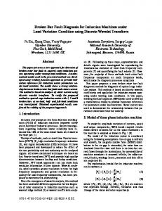
Fig.1.9 a) shows the amplitude of harmonic coefficients (h)LSR carried out for inductance lS1,R1(ϑ) shown in Fig.1.9 b). The series (1.2.5.7) contains only cosines terms, with phase 0o or 180o: phases can be discarded, by reversing (h)LSR signs. As it clearly appears, (h)LSR coefficients go to zero very rapidly with index h increasing: this is a very common property of cyclicsymmetric cage induction machines.

a)

b)

Fig.1.9. a): Inductance harmonic coefficients (h)LSR (10-5H on vertical axis). b): lS1,R1(ϑ) and gS1,R1(ϑ) = dlS1,R1(ϑ)/dϑ coefficients.

e) LSu,E, u = 1,…, n; are mutual inductances between a generic polar winding and one end-ring. They have the same constant negative value, since magnetic axes are always discordant; it results, obviously, LSu,E = LE,Su. f) LRk,E, k = 1,…, m; are mutual inductances between rotor loops and one end-ring. They have the same constant (negative) value, with LRk,E = LE,Rk. g) LE is the self-inductance of each cage end-ring.

36


1.2.6 – PSEUDO-INDUCTANCE MATRIX AND ELECTRO-MAGNETIC TORQUE By substituting the flux linkages expression (1.2.5.4) in (1.2.5.3), the “pseudo-inductance” matrix [g(ϑ)] compares:

[v(t )] = [R] ⋅ [i(t )] + [g (ϑ )] dϑ [i(t )] + [l (ϑ )] d [i(t )] dt

(1.2.6.1)

dt

where we have, for definition:

[g (ϑ )] = d [l (ϑ )]

(1.2.6.2)

dϑ

and, by performing a matrix partitioning:

[0] ⎡ [g(ϑ )] = ⎢⎢d[lRS (ϑ )]/ dϑ [0] ⎣⎢

d [lSR (ϑ )]/ dϑ

⎤ ⎡ [0] ⎥ = ⎢[g (ϑ )] ⎥ ⎢ RS ⎦⎥ ⎣⎢ [0]

[0] [0] [0]

[0] [0]

[gSR (ϑ)] [0] [0]

[0] [0] [0]

⎤ ⎥. ⎥ ⎦⎥

(1.2.6.3)

The sub-matrix [gSR(ϑ)] of (1.2.6.3) is structured as exposed in (1.2.6.4), (1.2.6.5). ⎡ g S 1, R1 (ϑ ) ⎢g ⎢ S 2, R1 (ϑ ) [g SR (ϑ )](nxm ) = ⎢ g S 3, R1 (ϑ ) ⎢ ⎢ ... ⎢ g Sn , R1 (ϑ ) ⎣

g Su , Rk (ϑ ) =

g S1, R 2 (ϑ )

g S 1, R 3 (ϑ )

...

g S 2, R 2 (ϑ ) g S 3, R 2 (ϑ )

g S 2, R 3 (ϑ ) g S 3, R 3 (ϑ )

... ...

...

...

...

g Sn , R 2 (ϑ )

g Sn , R 3 (ϑ )

...

g S 1, Rm (ϑ )⎤ g S 2, Rm (ϑ )⎥⎥ , g S 3, Rm (ϑ )⎥ ⎥ ... ⎥ g Sn, Rm (ϑ )⎥⎦

dlSu , Rk (ϑ ) ∞ = ∑ (− h )L(h ) sin{h[ϑ − (u − 1)δ S + (k − 1)δ R ]} . dϑ h =1

(1.2.6.4)

(1.2.6.5)

The “pseudo-inductance” matrix [g(ϑ)] permits to synthetically write the electromagnetic torque expression, as in (1.2.6.6).

Tem (ϑ , t ) =

1 [i(t )] T ⋅ [g (ϑ )] ⋅ [i(t )] . 2

(1.2.6.6)

In virtue of equation (1.2.6.3), we can reduce (1.2.6.6) to the following equivalent simplified forms, TSR and TRS:

Tem (ϑ , t ) = TSR = [iS (t )] ⋅ [g SR (ϑ )] ⋅ [iR (t )] ,

(1.2.6.7)

Tem (ϑ , t ) = TRS = [iR (t )] ⋅ [g RS (ϑ )] ⋅ [iS (t )] .

(1.2.6.8)

T

T

1.3 – THE (n,m+1) MODEL REDUCED FORM: THE (n,m) MODEL

The systems (1.2.5.1), (1.2.5.2) can be simplified if we assume that cage end-rings and stator windings are always healthy. In this case, in fact, the end-ring current iE(t) can be discarded from

37

Chapter 1 – The Squirrel Cage Induction Motor Phase Model the system, since it is constantly zero. This fact has a logical interpretation, bonded to the machine geometric symmetry, Fig.1.10. The end-ring loop current iE(t) virtually only flows in one end-ring: so, its presence denounces an asymmetry of current distribution between the two rings. This fact is justified if a ring is structurally altered with respect to the other (due to a damage or fracture); otherwise, an observer must see the same current distribution on the right and on the left side of the cage depicted in Fig.1.10, and iE(t) component must necessarily be zero in a healthy symmetrical machine. Another possible cause that makes rise the end-ring loop current is a stator winding defect or asymmetry, which produces a stator phase current homopolar component (current summation different from zero), as it can be deduced from eq. (1.2.4.2). This homopolar component appears in case of loss of ground insulation in three-wire connected three-phase windings, whereas in neutral-connected motors must be added, as possible causes, turn-to-turn or phase-to-phase short-circuits, or any other winding structural asymmetry. The relation between end-ring loop current, stator and rotor current homopolar components, air-gap field homopolar component, axial flux, and machine health status will be discussed and deepened in §2.3.5 of Chapter 2. In any case, the end-ring loop current must remain zero when bar breakages occur. In fact, a bar damage or interruption reduces (or annuls) a bar current, so the two contiguous loop currents become equal, and the effect is bilaterally symmetric on the opposite ring segments (stated that inter-bar currents are neglectable). Since in the following only bar breakages in a otherwise healthy machine will be considered, current iE(t) remains to zero, as its elimination from the model permits more simple transformations and mathematical manipulations. SYMMETRY AXIS

Fig.1.10. Bilateral symmetry for the current distribution in a healthy cage.

With the assumption iE(t)≡0 equations (1.2.5.1), (1.2.5.2) can be dimensionally reduced to (n+m) by (n+m) order, and we obtain the “(n,m) Model” of the induction machine: ⎡[vS (t )]⎤ ⎡[RSS ] ⎢[v (t )]⎥ = ⎢ [0] ⎣ R ⎦ ⎣

[0] ⎤ ⎡[iS (t )]⎤ d ⎡[ψ S (t )]⎤ ⋅ + [RRR ]⎥⎦ ⎢⎣[iR (t )]⎥⎦ dt ⎢⎣[ψ R (t )]⎥⎦

(1.3.1)

with flux linkages reassumed as follows: ⎡[ψ S (t )]⎤ ⎡[ψ SS (t )]⎤ ⎡[ψ SR (t )]⎤ ⎡ [LSS ] ⎢[ψ (t )]⎥ = ⎢[ψ (t )]⎥ + ⎢[ψ (t )]⎥ = ⎢[l (ϑ )] ⎣ R ⎦ ⎣ RS ⎦ ⎣ RR ⎦ ⎣ RS

[lSR (ϑ )]⎤ ⎡[iS (t )]⎤ . ⋅ [LRR ] ⎥⎦ ⎢⎣[iR (t )]⎥⎦

(1.3.2)

The electro-magnetic torque maintains the expression seen in (1.2.6.7), (1.2.6.8):

Tem (ϑ , t ) = [iS (t )] ⋅ [g SR (ϑ )]⋅ [i R (t )] . T

(1.3.3)

38


1.4 – THE SYMMETRICAL COMPONENTS TRANSFORMATION 1.4.1 – INTRODUCTION A useful transformation of the machine dynamic system (1.3.1)-(1.3.3) can be performed by using the Fortescue’s symmetrical components theory. The main advantage of machine equations transforming by using Fortescue’s matrices consists in the resistance and inductance matrices diagonalization, so obtaining a substantial mathematical simplification. The time-varying real variables (voltages, currents and flux linkages) of the original model go transformed to time-varying complex space vectors, and the machine dynamics can be decomposed in distinct but inter-dependent space sub-dynamics. If someone of these sub-dynamics can be discarded (because negligible), ulterior simplification can be gained, as it will be seen. 1.4.2 – CURRENT TRANSFORMATIONS Firstly, let consider a complex, reversible current transformation performed by using a Fortescue’s matrix of order n (that is a particular Vandermonde matrix), as in (1.4.2.1), where the real stator currents have been converted to complex space-vectors: ⎡1 ⎡ iS 1 (t )⎤ 1 ⎢ ⎢i (t )⎥ −1 ⎢ S 2 ⎥ 1 ⎢1 α S −2 ⎢ ⎢iS 3 (t )⎥ = 1 αS n⎢ ⎢ ⎥ ⎢M M ⎢ M ⎥ ⎢ −( n −1) ⎢⎣ iSn (t )⎥⎦ ⎣1 α S

1

α S −2 α S −4

1

K

α S −( n − 2 ) α S −2(n−2 )

K K

M

αS

− 2 ( n −1)

M

K αS

⎤ ⎡ iS (0 ) (t ) ⎤ ⎥ ⎢ (1) ⎥ α S −(n −1) ⎥ ⎢ iS (t ) ⎥ (2 ) α S −2 (n −1) ⎥ ⋅ ⎢ iS (t ) ⎥ ⎥ ⎢ ⎥ M ⎥ ⎢ M ⎥ 2 ( n −1) ⎥ α S −( n −1) ⎦ ⎢⎣iS (t )⎥⎦ 1

−( n − 2 )( n −1)

(1.4.2.1)

or, in a formally little different way, as in (1.4.2.2): ⎡1 ⎡ iS 1 (t )⎤ 1 1 ⎢ ⎢i (t )⎥ −1 −2 1 α α S S ⎢ S2 ⎥ 1 ⎢⎢ −2 ⎢iS 3 (t )⎥ = 1 αS α S −4 n⎢ ⎥ ⎢ M M ⎢M ⎢ M ⎥ ⎢1 α − ( n −1) α − 2( n −1) ⎢⎣ iSn (t )⎥⎦ S S ⎣

K K K

1

αS 2 αS 4

K αS

M

2 ( n −1)

⎤ ⎡ iS (0 ) (t ) ⎤ ⎥ ⎢ ⎥ α S ⎥ ⎢ iS (1) (t ) ⎥ α S 2 ⎥ ⋅ ⎢ iS (2 ) (t ) ⎥ ⎥ ⎢ ⎥ M ⎥ ⎢ M ⎥ α S ( n −1) ⎥⎦ ⎢⎣iS (−1) (t )⎥⎦ 1

(1.4.2.2)

where:

α S = e jδ . S

(1.4.2.3)

Equation (1.4.2.1) is formally more correct with respect to (1.4.2.2), but this one is more intuitive, since it points out the direct or reverse nature of the symmetrical systems that compose each column. Definition (1.4.2.1) for space vectors iS(q ) (t ) is not exhaustive, since it does not take in account index q values outside the range [0, n-1]. The definition (1.4.2.1) must be completed by introducing the following statement: iS(q ) (t ) = iS(q + k ⋅n ) (t ),

∀(q, k ) ∈ Ζ 2

(1.4.2.4)

where Z2 is the set that contains all the couple of relative integers. Equation (1.4.2.4) formally justifies the system (1.4.2.2). From now on, we not always will indicate explicitly the time-dependence (or angulardependence), accordingly to the convention of using lower-case letters for time-varying (or angular-varying) quantities, and upper-case letters for constant quantities, unless otherwise stated. Transformation (1.4.2.1) can be synthesized as follows:

39


[iS ] = [Fn ]⋅ [iS ']

(1.4.2.5)

The relation inverse of (1.4.2.1) is (1.4.2.6): ⎡ iS (0 ) (t ) ⎤ ⎡1 1 1 ⎢ (1) ⎥ ⎢ αS2 ⎢ iS (t ) ⎥ ⎢1 α S 1 ( ) 2 2 ⎢ i (t ) ⎥ = ⎢1 α αS4 S ⎢S ⎥ n⎢ M M ⎢ M ⎥ ⎢M ⎢i (−1) (t )⎥ ⎢1 α ( n −1) α 2 ( n −1) S S ⎣S ⎦ ⎣

1

K K

K αS

or:

−1

αS α S −4

K

M

⎤ ⎡ iS1 (t )⎤ ⎥ ⎢ ⎥ α S ⎥ ⎢iS 2 (t )⎥ −2 ⎥ ⋅ ⎢iS 3 (t )⎥ αS ⎥ ⎢ ⎥ M ⎥ ⎢ M ⎥ α S − ( n −1) ⎥⎦ ⎢⎣ iSn (t )⎥⎦ 1

−2

− 2 ( n −1)

∗

[iS '] = [Fn ] ⋅ [iS ]

(1.4.2.6)

(1.4.2.7)

in matrix form, where the asterisk denotes a complex-conjugate quantity. Current space-vectors as defined in (1.4.2.6) are complex conjugate in pairs:

iS

(q )

= iS

(− q )

(1.4.2.8)

*

An analogous transformation can be performed on the rotor currents, by using a Fortescue’s matrix of order m: ⎡1 ⎡ iR1 (t ) ⎤ 1 1 ⎢ ⎢ i (t )⎥ −1 1 αR α R−2 ⎢ R2 ⎥ 1 ⎢⎢ −2 ⎢ iR 3 (t )⎥ = 1 αR α R−4 m⎢ ⎢ ⎥ M M ⎢M ⎢ M ⎥ ⎢1 α − ( m −1) α − 2 ( m −1) ⎢⎣iRm (t )⎥⎦ R R ⎣

1

K

αR α R4

K K

K αR

⎤ ⎡ iR (0 ) (t ) ⎤ ⎥ ⎢ ⎥ α R ⎥ ⎢ iR (1) (t ) ⎥ α R 2 ⎥ ⋅ ⎢ iR (2 ) (t ) ⎥ ⎥ ⎢ ⎥ M ⎥ ⎢ M ⎥ α R ( m −1) ⎥⎦ ⎢⎣iR (−1) (t )⎥⎦ 1

2

M

2 ( m −1)

(1.4.2.9)

where:

α R = e jδ . R

(1.4.2.10)

The matrix form for transformation (1.4.2.9) is:

[iR ] = [Fm ]⋅ [iR '] .

(1.4.2.11)

The relation inverse of (1.4.2.11) is (1.4.2.12):

∗

[iR '] = [Fm ] ⋅ [iR ] .

(1.4.2.12)

1.4.3 – VOLTAGE AND FLUX TRANSFORMATIONS By substituting equations (1.4.2.5), (1.4.2.11) into systems (1.3.1), (1.3.2), we obtain: ⎡[vS ]⎤ ⎡[RSS ] ⋅ [Fn ] ⎢[v ]⎥ = ⎢ [0] ⎣ R⎦ ⎣

[0] ⎤ ⎡[iS ']⎤ d ⎡[ψ S ]⎤ ⋅ + [RRR ] ⋅ [Fm ]⎥⎦ ⎢⎣[iR ']⎥⎦ dt ⎢⎣[ψ R ]⎥⎦

(1.4.3.1)

for the voltage expressions, and:

40

Chapter 1 – The Squirrel Cage Induction Motor Phase Model ⎡[ψ S ]⎤ ⎡ [LSS ]⋅ [Fn ] ⎢[ψ ]⎥ = ⎢[l (ϑ )]⋅ [F ] n ⎣ R ⎦ ⎣ RS

[lSR (ϑ )]⋅ [Fm ]⎤ ⎡[iS ']⎤ , ⋅ [LRR ]⋅ [Fm ] ⎥⎦ ⎢⎣[iR ']⎥⎦

(1.4.3.2)

for the flux linkage expressions. By multiplying the first equations of the systems (1.4.3.1) and (1.4.3.2) by [Fn]* and the second equations by [Fm]*, we easily obtain systems (1.4.3.3), (1.4.3.4): ∗ ∗ ⎤ ⎡ ⎡ ⎢ [Fn ] ⋅ [vS ]⎥ ⎢[Fn ] ⋅ [RSS ] ⋅ [Fn ] ⎥=⎢ ⎢ ⎢[F ]∗ ⋅ [v ]⎥ ⎢ [0] R ⎥ ⎢⎣ m ⎦ ⎢⎣

⎤ ⎡ ⎥ ⎢[iS '] ⎥⋅⎢ ∗ [Fm ] ⋅ [RRR ]⋅ [Fm ]⎥⎥ ⎢⎢[iR '] ⎦ ⎣

[0]

∗ ∗ ⎡ ⎤ ⎡ ⎢ [Fn ] ⋅ [ψ S ]⎥ ⎢ [Fn ] ⋅ [LSS ]⋅ [Fn ] ⎢ ⎥=⎢ ⎢[F ]∗ ⋅ [ψ ]⎥ ⎢[F ]∗ ⋅ [l (ϑ )]⋅ [F ] R ⎥ m RS n ⎢⎣ m ⎦ ⎢⎣

∗ ⎤ ⎡ ⎤ ⎥ d ⎢ [Fn ] ⋅ [ψ S ]⎥ , ⎥ ⎥+ ⎢ ⎥ dt ⎢[F ]∗ ⋅ [ψ ]⎥ R ⎥ ⎢⎣ m ⎥⎦ ⎦

(1.4.3.3)

∗

[Fn ] ⋅ [lSR (ϑ )]⋅ [Fm ]⎤⎥ ⎡⎢[iS '] ⎤⎥ . ⎥⋅⎢ ⎥ ∗ [Fm ] ⋅ [LRR ]⋅ [Fm ] ⎥⎥ ⎢⎢[iR '] ⎥⎥ ⎦ ⎣

(1.4.3.4)

⎦

Note that in (1.4.3.3) the time-invariance of matrices [Fn ] , [Fm ] , has been exploited. This is one of the important reasons for using classical Fortescue’s matrices: infact, generally time-variable transformations introduce ulterior terms when derived, which add more complexity to the model. So, it clearly appears that by transforming voltages and flux linkages by exploiting the same transformations used for the currents, i.e.:

∗

[vS ] = [Fn ]⋅ [vS ']

and

[vS '] = [Fn ] ⋅ [vS ] ,

[vR ] = [Fm ] ⋅ [vR ']

and

[vR '] = [Fm ] ⋅ [vR ],

[ψ S ] = [Fn ]⋅ [ψ S ']

and

[ψ S '] = [Fn ] ⋅ [ψ S ] ,

[ψ R ] = [Fm ] ⋅ [ψ R ']

and

[ψ R '] = [Fm ] ⋅ [ψ R ] ,

∗

(1.4.3.5) (1.4.3.6)

for voltages, and

∗

∗

(1.4.3.7) (1.4.3.8)

for flux linkages, we gain the twofold vantage of obtaining two systems (1.4.3.9), (1.4.3.10) formally identical to the original untransformed ones, but with diagonalized matrices: ⎡[vS ']⎤ ⎡[RSS '] ⎢[v ']⎥ = ⎢ [0] ⎣ R ⎦ ⎣

[0] ⎤ ⎡[iS ']⎤ d ⎡[ψ 'S ]⎤ , ⋅ + [RRR ']⎥⎦ ⎢⎣[iR ']⎥⎦ dt ⎢⎣[ψ 'R ]⎥⎦

(1.4.3.9)

[l ' (ϑ )]⎤ ⎡[i ']⎤ ] [L '] ⎥⎦ ⋅ ⎢⎣[i ']⎥⎦

(1.4.3.10)

⎡[ψ S ']⎤ ⎡ [LSS '] ⎢[ψ ']⎥ = ⎢ ⎣ R ⎦ ⎣ lRS ' (ϑ )

[

S

SR

RR

R

where voltage, current, and linked flux transformed column vectors are the followings:

41

Chapter 1 – The Squirrel Cage Induction Motor Phase Model ⎡ vS(0 ) (t ) ⎤ ⎢ (1) ⎥ ⎢ vS (t ) ⎥ ; [vS ' (t )](nx1) = ⎢ vS(2 ) (t ) ⎥ ⎢ ⎥ ⎢ ... ⎥ ⎢v (−1) (t )⎥ ⎣ S ⎦

⎡ iS(0 ) (t ) ⎤ ⎢ (1) ⎥ ⎢ iS (t ) ⎥ ; [iS ' (t )](nx1) = ⎢ iS(2 ) (t ) ⎥ ⎥ ⎢ ⎢ ... ⎥ ⎢i (−1) (t )⎥ ⎦ ⎣S

⎡ψ S(0 ) (t ) ⎤ ⎢ (1) ⎥ ⎢ ψ S (t ) ⎥ ; [ψ S ' (t )](nx1) = ⎢ψ S(2 ) (t ) ⎥ ⎢ ⎥ ⎢ ... ⎥ ⎢ψ (−1) (t )⎥ ⎣ S ⎦

⎡ vR(0 ) (t ) ⎤ ⎢ (1) ⎥ ⎢ vR (t ) ⎥ ; [vR ' (t )](mx1) = ⎢ vR(2 ) (t ) ⎥ ⎥ ⎢ ⎢ ... ⎥ ⎢v (−1) (t )⎥ ⎦ ⎣ R

⎡ iR(0 ) (t ) ⎤ ⎢ (1) ⎥ ⎢ iR (t ) ⎥ ; [iR ' (t )](mx1) = ⎢ iR(2 ) (t ) ⎥ ⎥ ⎢ ⎢ ... ⎥ ⎢i (−1) (t )⎥ ⎦ ⎣R

⎡ψ R(0 ) (t ) ⎤ ⎢ (1) ⎥ ⎢ ψ R (t ) ⎥ . = ⎢ψ R(2 ) (t ) ⎥ ⎥ ⎢ ⎢ ... ⎥ ⎢ψ (−1) (t )⎥ ⎦ ⎣ R

[ψ R ' (t )](mx1)

(1.4.3.11)

(1.4.3.12)

The followings identities hold true for transformed matrices: ⎡ ⎢[RSS '] ⎢ ⎢ [0] ⎢⎣ ⎡ ⎢ [LSS '] ⎢ ⎢ l ' (ϑ ) ⎢⎣ RS

[

]

∗ ⎤ ⎡ ⎥ ⎢[Fn ] ⋅ [RSS ] ⋅ [Fn ] ⎥=⎢ [RRR ']⎥⎥ ⎢⎢ [0] ⎦ ⎣

[0]

⎤ ⎥, ⎥ ∗ [Fm ] ⋅ [RRR ]⋅ [Fm ]⎥⎥ ⎦

∗ ⎡ ⎢ [Fn ] ⋅ [LSS ]⋅ [Fn ] ⎥=⎢ ∗ [LRR '] ⎥⎥ ⎢⎢[Fm ] ⋅ [l RS (ϑ )]⋅ [Fn ] ⎦ ⎣

[l ' (ϑ )]⎤⎥ SR

[0]

(1.4.3.13)

∗

[Fn ] ⋅ [lSR (ϑ )]⋅ [Fm ]⎤⎥ . ∗

[Fm ]

(1.4.3.14)

⎥ ⋅ [LRR ]⋅ [Fm ] ⎥ ⎥⎦

The transformed flux linkage column vectors [ψ S '] and [ψ R '] can be decomposed as done with the original ones in (1.3.2): ⎡ ⎢[ψ S '] ⎢ ⎢[ψ '] ⎢⎣ R

∗ ∗ ⎤ ⎡ ⎤ ⎡ ⎤ ⎡ ⎥ ⎢ [Fn ] ⋅ [ψ SS (t )]⎥ ⎢ [Fn ] ⋅ [ψ SR (t )]⎥ ⎢[ψ SS '] ⎥=⎢ ⎥+⎢ ⎥=⎢ ⎥ ⎢[F ]∗ ⋅ [ψ (t )]⎥ ⎢[F ]∗ ⋅ [ψ (t )]⎥ ⎢[ψ '] RS RR ⎥⎦ ⎢⎣ m ⎥⎦ ⎢⎣ m ⎥⎦ ⎢⎣ RS

⎤ ⎡ ⎥ ⎢[ψ SR '] ⎥+⎢ ⎥ ⎢[ψ '] ⎥⎦ ⎢⎣ RR

⎤ ⎥ ⎥ ⎥ ⎥⎦

(1.4.3.15)

and obviously we get: ⎡[ψ SS ']⎤ ⎡[ψ SR ']⎤ ⎡ [LSS '] ⎢[ψ ']⎥ + ⎢[ψ ']⎥ = ⎢ ⎣ RS ⎦ ⎣ RR ⎦ ⎣ lRS ' (ϑ )

[

]

[l ' (ϑ )]⎤ ⋅ ⎡[i ' (t )]⎤ .

(1.4.3.16)

S

SR

[LRR '] ⎥⎦ ⎢⎣[iR ' (t )]⎥⎦

Reverse relations of (1.4.3.15) are written as: ⎡[ψ S ]⎤ ⎡ [Fn ]⋅ [ψ SS ']⎤ ⎡ [Fn ]⋅ [ψ SR ']⎤ ⎡[ψ SS ]⎤ ⎡[ψ SR ]⎤ . ⎢[ψ ]⎥ = ⎢[F ]⋅ [ψ ']⎥ + ⎢[F ]⋅ [ψ ']⎥ = ⎢[ψ ]⎥ + ⎢[ψ ]⎥ RS ⎦ RR ⎦ ⎣ R⎦ ⎣ m ⎣ m ⎣ RS ⎦ ⎣ RR ⎦

(1.4.3.17)

[ ]

[ ]

The transformed mutual stator-rotor inductance matrices as defined in (1.4.3.14), lSR ' and lRS ' , are Hermitian transpose matrices each one for the other, that is:

[l '] = [l ']

T

RS

SR

∗

[ ]

= lSR '

H

(1.4.3.18)

since the same property is true for the un-transformed (real) matrices:

42


[l RS ] = [lSR ]

T

∗

= [l SR ]

H

(1.4.3.19)

1.4.4 – PSEUDO-INDUCTANCE MATRIX AND ELECTRO-MAGNETIC TORQUE TRANSFORMATIONS The pseudo-inductance matrix (1.2.6.3) undergoes transformation too, thus allowing more synthetic expressions. By substituting the transformed fluxes (1.4.3.10) into the transformed electric balance (1.4.3.9), a new dynamical expression for transformed machines can be gained as in formula (1.4.4.1). ⎡ [RSS '] + [LSS '] p ⎡[vS ']⎤ ⎢ ⎢[v ']⎥ = ⎢ ⎣ R ⎦ ⎢[g RS ' (ϑ )] dϑ + lRS ' (ϑ ) p dt ⎣

[

]

[g SR ' (ϑ )] dϑ + [lSR ' (ϑ )]p ⎤⎥ ⎡[iS ']⎤ . dt ⎥⋅⎢ ⎥ [RRR '] + [LRR '] p ⎥ ⎣[iR ']⎦

(1.4.4.1)

⎦

In (1.4.4.1) the transformed mutual pseudo-inductance matrices have been introduced, defined as angular derivative of the correspondent transformed inductance matrices, or equivalently as transformations of the original pseudo-inductance matrices, (1.4.4.2). ⎡ ⎢ [0] ⎢ ⎢ [g ' (ϑ )] ⎢⎣ RS

[g SR ' (ϑ )]⎤⎥ [0]

⎡ ⎢ [0] ⎥=⎢ ⎥ ⎢ d l RS ' (ϑ ) ⎥⎦ ⎣⎢ dϑ

[

]

[

]

d l SR ' (ϑ ) ⎤ ⎡ [0] ⎥ ⎢ dϑ ⎥ = ⎢ ∗ [0] ⎥⎥ ⎢⎢[Fm ] [g RS (ϑ)]⋅ [Fn ] ⎦ ⎣

∗

[Fn ] [g SR (ϑ)]⋅ [Fm ]⎤⎥ . (1.4.4.2) ⎥ ⎥ [0] ⎥ ⎦

The pseudo-inductance matrices and their transformed are Hermitian transpose matrices each one for the other:

[g RS ] = [g SR ]

T

∗

= [g SR ] ,

T

∗

= [g SR '] .

[g RS '] = [g SR ']

H

H

(1.4.4.3) (1.4.4.4)

The transformed complex expressions for the electro-magnetic torque can be easily carried out by starting from definition (1.4.4.5): Tem (ϑ , t ) =

1 ⎡[iS ]⎤ 2 ⎢⎣[iR ]⎥⎦

H

⎡ [0] ⋅⎢ ⎣[g RS ]

[g SR ]⎤ ⎡[iS ]⎤ ⋅ [0] ⎥⎦ ⎢⎣[iR ]⎥⎦

(1.4.4.5)

that can be reduced to two different equivalent forms, TSR and TRS: H

Tem (ϑ , t ) = TSR = [iS ] ⋅ [g SR ] ⋅ [iR ] , H

Tem (ϑ , t ) = TRS = [iR ] ⋅ [g RS ] ⋅ [iS ] .

(1.4.4.6)

(1.4.4.7)

By using the definitions (1.4.2.5), (1.4.2.11), and (1.4.4.2), from (1.4.4.6) and (1.4.4.7) the followings alternative expressions can be obtained: H

Tem (ϑ , t ) = TSR = [iS '] ⋅ [g SR '] ⋅ [iR '] , H

Tem (ϑ , t ) = TRS = [iR '] ⋅ [g RS '] ⋅ [iS '] .

(1.4.4.8) (1.4.4.9)

43

Chapter 1 – The Squirrel Cage Induction Motor Phase Model 1.5 – TRANSFORMATIONS FOR CIRCULATING MATRICES 1.5.1 – INTRODUCTION As previously pointed out, the Fortescue’s transformations permit to put in diagonal form resistance and inductance matrices, if they are “circulant” matrices (see Appendix 1.A). Moreover, the matrices [RSS], [RRR], [LSS], [LRR] of model (1.3.1), (1.3.2) are circulant, real and symmetric (see Def.3 of §1.A.1), so the transformation produces diagonal matrices with real elements matched orderly in pairs (see §1.A.3.3). By using formula (1.A.3.3.6), we can transform the aforementioned matrices. 1.5.2 – TRANSFORMATION OF [RSS] Transformation (1.5.2.1) derives from (1.4.3.13) and it is immediate, since [RSS] is diagonal:

∗

[RSS '] = [Fn ] ⋅ [RSS ]⋅ [Fn ]

(1.5.2.1)

and it produces a real diagonal transformed matrix:

[RSS '] = [RSS ] .

(1.5.2.2)

By writing the expanded form of (1.5.2.2) we get: ⎡ ⎢ ⎢ ⎢ [RSS '](nxn ) = ⎢ ⎢ ⎢ ⎢ ⎣⎢

with

RS(0 ) 0 0 ... 0

0 RS(1) 0 ... 0

0 0 RS(2 ) ... 0

... ... ... ... ...

RS(n − 2 )

0

0

0

...

0

RS(u ) = RS ,

0 0 0 ...

⎤ ⎥ ⎥ ⎥ ⎥ ⎥ ⎥ ⎥ RS(n −1) ⎦⎥ 0 0 0 ... 0

u = 0,..., n − 1 .

(1.5.2.3)

(1.5.2.4)

1.5.3 – TRANSFORMATION OF [RRR] Transformation (1.5.3.1) of matrix (1.2.3.7) is derived from (1.4.3.13):

∗

[RRR '] = [Fm ] ⋅ [RRR ] ⋅ [Fm ] .

(1.5.3.1)

By applying (1.A.3.3.6), formulas (1.5.3.2)-(1.5.3.3) can be readily obtained. ⎡ ⎢ ⎢ ⎢ [RRR '](mxm ) = ⎢ ⎢ ⎢ ⎢ ⎣⎢

RR(0 ) 0 0 ... 0 0

0 RR(1) 0 ... 0 0

0 0 RR(2 ) ... 0 0

... ... ... ... ... ...

0 0 0 ... RR(m − 2 ) 0

⎤ ⎥ ⎥ ⎥ ⎥ ⎥ ⎥ ⎥ (m −1) RR ⎦⎥ 0 0 0 ... 0

(1.5.3.2)

with real elements:

44

Chapter 1 – The Squirrel Cage Induction Motor Phase Model RR(k ) = 2[RB (1 − cos kδ R ) + RE / m],

Note that:

RR(k ) = RR(m − k ) ,

k = 0,..., m − 1 .

k = 1,..., m − 1 .

(1.5.3.3)

(1.5.3.4)

1.5.4 – TRANSFORMATION OF [LSS] Transformation of matrix (1.2.2.6) derived from (1.4.3.14) is (1.5.4.1):

∗

[LSS '] = [Fn ] ⋅ [LSS ] ⋅ [Fn ] .

(1.5.4.1)

By applying definition (1.A.3.3.6) on the elements of (1.2.5.5), we obtain the matrix (1.5.4.2), with real elements (1.5.4.3), which have the properties (1.5.4.4). ⎡ ⎢ ⎢ ⎢ [LSS '](nxn ) = ⎢ ⎢ ⎢ ⎢ ⎣⎢

L(S0 )

0

0

...

0

0 0 ... 0 0

(1)

LS 0 ... 0 0

0 L(S2 ) ... 0 0

... ... ... ... ...

0 0 ...

n −1

L(Su ) = ∑ Lwδ S ⋅ cos(wuδ S ),

L(Sn − 2 ) 0

0 ⎤ ⎥ 0 ⎥ 0 ⎥; ⎥ ... ⎥ 0 ⎥ ⎥ (n −1) LS ⎦⎥

u = 0,..., n − 1 ;

(1.5.4.2)

(1.5.4.3)

w=0

L(Su ) = L(Sn −u ) ,

u = 1,..., n − 1 .

(1.5.4.4)

1.5.5 – TRANSFORMATION OF [LRR] Transformation of matrix (1.2.3.12) derived from (1.4.3.14) is (1.5.5.1):

∗

[LRR '] = [Fm ] ⋅ [LRR ] ⋅ [Fm ].

(1.5.5.1)

By applying definition (1.A.3.3.6) on the elements of (1.2.5.6), we obtain (1.5.5.2)-(1.5.5.4) (real elements). ⎡ ⎢ ⎢ ⎢ [LRR '](mxm ) = ⎢ ⎢ ⎢ ⎢ ⎢⎣

L(R0 ) 0 0 ... 0 0

0 L(R1) 0 ... 0 0

m −1

0 0 L(R2 ) ... 0 0

... ... ... ... ... ...

L(Rk ) = ∑ Lwδ R ⋅ cos(wkδ R ),

0 0 0 ... L(Rm − 2 ) 0

⎤ ⎥ ⎥ ⎥; ⎥ ⎥ ⎥ ⎥ ( m −1) LR ⎥⎦ 0 0 0 ... 0

k = 0,..., m − 1 ;

(1.5.5.2)

(1.5.5.3)

w=0

L(Rk ) = L(Rm − k ) ,

k = 1,..., m − 1 .

(1.5.5.4)

45

Chapter 1 – The Squirrel Cage Induction Motor Phase Model 1.6 – TRANSFORMATION OF GENERIC ASYMMETRICAL MUTUAL INDUCTANCE RECTANGULAR MATRICES BY MEANS OF BI-SYMMETRICAL COMPONENTS 1.6.1 – INTRODUCTION The Fortescue transformations applied to a generic (nxm) rectangular matrix whose elements are time or space iso-frequency sinusoidal functions permit computation of the correspondent “bisymmetrical” component systems (see Appendix 1.B). The mutual stator-rotor inductance matrices [lSR(ϑ)] and [lRS(ϑ)] with elements defined as in (1.2.5.7) for a cyclic-symmetric machine gain a great formal simplification when transformations like those reported in (1.4.3.14) have been performed. In this paragraph a general presentation of bi-symmetrical components theory applied to any asymmetric periodic mutual inductance matrix will be given, in order to introduce appropriate symbolisms and to state the principal properties and virtues of such a technique. In the next paragraph the actual transformation for a cyclic-symmetric machine will be introduced. 1.6.2 – MUTUAL INDUCTANCE MATRIX COMPLEX FORM To perform transformation of [lSR(ϑ)] in the easier way, it is suitable putting it in a more general complex form. Let consider the following generic real unilateral Fourier harmonic decomposition (see Appendix 1.C for details):

[lSR ] = ∑ [(h )lSR ] ∞

(1.6.2.1)

h =0

with h order harmonic component matrices (unilateral terms) defined as follows:

[( )l ]( h

SR

=

nxm )

{( )l } = {( ) L h

h

SuRk uk

SuRk

(

)}

cos hϑ − (h )η SuRk , h ∈ N 0

(1.6.2.2)

(note N0 is the set containing all natural integer numbers, including zero). The definitions (1.6.2.1), (1.6.2.2) are much more general than (1.2.5.7), since in (1.6.2.2) each harmonic component of the mutual inductance coefficient related to uth stator circuit and to kth rotor circuit is a cosines function with arbitraries amplitude and phase. Positions (1.6.2.1), (1.6.2.2), correspond to a rotating machine with a completely asymmetric circuit distribution, that is, matrix (1.6.2.2) is a generic un-bisymmetric system. The complex variable-phasor representation of matrix (1.6.2.2) is (1.6.2.3):

[( )~l ]( h

SR

nxm )

=

{( )~l } = {( )L h

h

SuRk uk

SuRk

}

(1.6.2.3)

}

(1.6.2.4)

h ∈ N0 .

(1.6.2.5)

e j (hϑ −

( h )η

SuRk

) , h∈ N 0

whereas the complex constant-phasor representation is (1.6.2.4).

[( ) L ]( h

SR

nxm )

It results:

=

{( ) L } h

SuRk uk

=

{

(h )

[( )~l ] = [( )L ] e h

h

SR

SR

LSuRk e − j (

jhϑ

,

( h )η

SuRk

) , h∈ N . 0

The summation (1.6.2.1) can be extended to h∈Z, to obtain more compact formal results. A real bilateral Fourier series (see §1.C.2) can be made up in matrix form by summing terms (bilateral terms) like those reported in definition (1.6.2.6):

[( )λ ]( h

SR

nxm )

=

{( )λ } = {( )Λ h

h

SuRk uk

SuRk

(

)}

cos hϑ − (h )ξ SuRk ,

h∈Z

(1.6.2.6)

46

Chapter 1 – The Squirrel Cage Induction Motor Phase Model where unknown amplitudes and phases must be related to those in (1.6.2.2) by means of the following relations: ⎧ (h )Λ SuRk = (h )LSuRk / 2 ; ⎨ (h ) (h ) ⎩ ξ SuRk = η SuRk ⎧ (0 )Λ SuRk = (0 )LSuRk cos (0 )η SuRk ; ⎨ (0 ) ⎩ ξ SuRk = 0 ⎧ (− h )Λ SuRk = (h )LSuRk / 2 ; ⎨ ( −h ) (h ) ξ =− η SuRk SuRk ⎩

h∈ N :

(

h = 0: h∈ N :

)

(1.6.2.8) (1.6.2.9)

k = 1,..., m .

u = 1,..., n ;

for

(1.6.2.7)

From (1.6.2.6)-(1.6.2.9) it can be easily proved that the properties (1.6.2.10)-(1.6.2.12) hold true.

[( )λ ] = [(

−h)

h∈Z :

⎧ (h )Λ SuRk = (− h )Λ SuRk ; ⎨ (h ) (− h ) ξ =− ξ SuRk ⎩ SuRk

[( )λ ] + [(

−h)

h

SR

h

SR

λSR ] ,

h∈Z ;

λSR ] = [(h )lSR ] ,

[( )λ ] = [( )l ], 0

0

SR

SR

(1.6.2.10) (1.6.2.10’)

h∈ N ;

(1.6.2.11)

h = 0.

(1.6.2.12)

From (1.6.2.11), (1.6.2.12), (1.6.2.1), the real bilateral Fourier series development of [lSR] immediately descends:

[lSR ] = ∑ [(h )λSR ]. ∞

(1.6.2.13)

h=−∞

By definition, (1.6.2.14) furnishes the elements of matrix phasor form associated to matrix (1.6.2.6).

[( )λ~ ]( h

SR

nxm )

=

{( )λ~ } = {( )Λ h

h

SuRk uk

SuRk

e j (hϑ −

[( )λ~ ], that is the complex variable-

( h )ξ

h

SR

SuRk

}

) ,

h∈Z .

(1.6.2.14)

Obviously it results:

[( )λ ] = Re([( )λ~ ]) ,

h∈Z .

(1.6.2.15)

[( )λ~ ] = [(

h∈Z ;

(1.6.2.16)

λSR = [(h )lSR ], h ∈ N ;

(1.6.2.17)

h

h

SR

SR

Note that: h

SR

[( )λ~ ]+ [( h

SR

−h)

−h)

~

]

[( )λ~ ] = [( )l ], 0

0

SR

SR

]

~ ∗

λSR ,

h = 0.

(1.6.2.18)

47


From (1.6.2.17), (1.6.2.18) and (1.6.2.1) we obtain the complex bilateral Fourier series development of [lSR]:

[lSR ] = ∑ [(h )λ~SR ]. ∞

(1.6.2.19)

h = −∞

By considering that (1.6.2.2) is the real part of (1.6.2.3), series (1.6.2.1) becomes:

[lSR ] = ∑ [ ∞

( h )~

][ ]

~ lSR + (h )lSR * ∞ =∑ 2 h =1

h =0

[( )~l ] + [( )~l ]+ [( )~l ]* + ∑ [( h

0

SR

0

SR

2

∞

SR

2

h =−1

]

~ lSR * 2

−h)

(1.6.2.20)

and, by identifying correspondent terms of (1.6.2.20) and (1.6.2.19), we get the following relations:

[( )λ~ ] = 12 [( )~l ], h

h

SR

[(

−h)

SR

] 12 [( )~l ]* ,

~

λSR =

h

SR

h∈ N ;

(1.6.2.21)

h∈ N ;

(1.6.2.22)

( )~ ( )~ [( )λ~ ] = [ l ]+2[ l ]* , h = 0 . 0

0

0

SR

SR

(1.6.2.23)

SR

By separating constant and variable parts of (1.6.2.14), we gain:

[( )λ~ ] = [( )Λ ] e h

h

SR

SR

jhϑ

, h∈Z

(1.6.2.24)

where the following complex constant-phasor representation was introduced:

[( )Λ ]( h

SR

nxm )

=

{( )Λ } h

SuRk uk

=

{

Λ SuRk e − j (

(h )

( h )ξ

SuRk

}

) ,

h∈Z

(1.6.2.25)

with expanded form as follows: ⎡ (h )Λ S1R1 ⎢ (h ) ⎢ Λ S 2 R1 ⎢ (h )Λ S 3 R1 (nxm ) = ⎢ ⎢ ... ⎢ (h )Λ SnR1 ⎣

SR

(h ) (h )

Λ S 1R 2

ΛS 2R2 (h ) ΛS 3R 2 ... (h ) Λ SnR 2

[( )Λ ] h

(h ) (h )

Λ S 1R 3

...

ΛS 2R3 (h ) Λ S 3R 3 ... (h ) Λ SnR 3

... ... ... ...

(h )

Λ S 1Rm ⎤ ⎥ Λ S 2 Rm ⎥ , (h ) Λ S 3 Rm ⎥ ⎥ ... ⎥ (h ) Λ SnRm ⎥⎦

(h )

h∈Z .

(1.6.2.26)

By exploiting the relations (1.6.2.5) and (1.6.2.24), the relations (1.6.2.21), (1.6.2.22), (1.6.2.23) assume the alternative form as follows:

[( )Λ ] = [

(h )

h

SR

[(

−h)

]

LSR , 2

( ) ] [ L2 ]* ,

Λ SR =

h

SR

h∈ N ;

(1.6.2.27)

h∈ N ;

(1.6.2.28)

48


[( )Λ ]( 0

SR nxm )

=

[( )L ]+ [( )L ]* = [( )l ], 2 0

0

SR

h=0.

0

SR

SR

(1.6.2.29)

From (1.6.2.27)-(1.6.2.29) the property (1.6.2.30) can be carried out:

[( )Λ ] = [( h

SR

−h )

Λ SR

]∗ ,

h∈Z .

(1.6.2.30)

The definition (1.6.2.24) can be substituted in (1.6.2.19), so producing a new equivalent expression for [lSR]:

[lSR ] = ∑ [(h )Λ SR ] e jhϑ ∞

(1.6.2.31)

h = −∞

or, by expanding terms:

[lSR ] = ... + [(−2)ΛSR ]e− j 2ϑ + [(−1)ΛSR ]e− jϑ + [(0)ΛSR ]+ [(1)ΛSR ]e jϑ + [(2)ΛSR ]e j 2ϑ + ...

[

(1.6.2.32)

]

Note that the complex matrices (h )Λ SR contain amplitudes and phases of the real asymmetrical systems (1.6.2.6), thus preserving information. The expressions (1.6.2.19), (1.6.2.24), and (1.6.2.31) will be useful to perform transformation in the next paragraphs. 1.6.3 – MUTUAL INDUCTANCE MATRIX TRANSFORMATION The transformation of the matrix [lSR(ϑ)] introduced by equation (1.4.3.14) can be better accomplished by exploiting the complex bilateral definition (1.6.2.19) together with relation (1.6.2.24) (merged in (1.6.2.31)). In fact, in this way, the transformation of the real matrix [lSR] can be performed by simply transforming some constant complex matrices, and the formula (1.B.4.10) containing the correspondent bisymmetrical components can be directly employed to gain a synthetic result. From (1.4.3.14) we have the following definition:

[l '] = [F ]∗ ⋅ [l ]⋅ [F ] SR

n

SR

(1.6.3.1)

m

[ ]

where the transformed complex matrix lSR ' has been introduced, with structure defined as explicitly reported in (1.6.3.2).

[l ']( SR

nxm )

{

= lSR( p , q )

}

pq

⎡ lSR(0,0 ) lSR(0,1) lSR(0, 2 ) ⎢ (1,0 ) lSR(1,1) lSR(1, 2 ) ⎢ lSR 2 , 0 2 , 1 ( ) ( ) = ⎢ lSR lSR lSR(2, 2 ) ⎢ ... ... ⎢ ... ⎢l (n −1,0 ) l (n −1,1) l (n −1, 2 ) SR SR ⎣ SR

lSR(0, m −1) ⎤ ⎥ lSR(1, m −1) ⎥ . ... lSR(2, m −1) ⎥ ⎥ ... ... ⎥ ... lSR(n −1, m −1) ⎥⎦ ... ...

(1.6.3.2)

The computation of the elements of (1.6.3.2) is directly performed by exploiting relation (1.6.2.31), that furnishes an expression for [lSR] usable in (1.6.3.1):

[l '] = ∑ [F ]∗ ⋅ [( )Λ ]⋅ [F ] e ∞

SR

h

n

SR

m

jhϑ

.

(1.6.3.3)

h = −∞

49


The right-member in (1.6.3.3) contains terms of type (1.B.4.10), so a complex bi-symmetrical component matrix can be introduced for each one of the complex asymmetrical matrix systems

[( )Λ ] as follows: h

SR

[( )Λ '] = [F ]∗ ⋅ [( )Λ ]⋅ [F ], h

h∈Z

h

SR

n

SR

m

(1.6.3.4)

thus obtaining the following synthetic transformed form for (1.6.3.1):

[l '] = ∑ [( )Λ '] e ∞

h

SR

SR

jhϑ

.

(1.6.3.5)

h =−∞

[( )Λ '] contains all the bisymmetrical components of h

As stated in Appendix 1.B, the matrix the system (1.B.4.11).

[

(h )

SR

]

Λ SR , and its explicit form is furnished in (1.6.3.6) similarly to that in equation

[( )Λ ']( h

SR

nxm )

0, 0 ) ⎡ (h )Λ(SR ⎢ (h ) (1,0 ) ⎢ Λ SR 2, 0 ) = ⎢ (h )Λ(SR ⎢ ⎢ ... ⎢ (h )Λ(n−1,0 ) SR ⎣

( h ) (0,1)

Λ SR

( h ) (0 , 2 )

...

( h ) (1,1)

Λ SR

Λ SR Λ SR ... (h ) ( n −1,1) Λ SR

( h ) (1, 2 )

Λ SR Λ SR ... (h ) ( n −1, 2 ) Λ SR

... ... ... ...

(h ) (2 ,1)

(h ) (2, 2 )

( h ) (0 ,m −1)

⎤ ⎥ Λ SR ⎥ , ( h ) (2 ,m −1) ⎥ Λ SR ⎥ ... ⎥ (h ) ( n −1,m−1) ⎥ Λ SR ⎦ Λ SR

( h ) (1,m −1)

h∈Z

(1.6.3.6)

or, more synthetically:

[( )Λ ']( h

SR

nxm )

=

{( )Λ( )} h

p,q SR

pq

=

{Λ

(h ) ( p , q ) SR

e− j

( ( )ξ ( ) ) h

p ,q SR

}

pq

, h∈Z .

(1.6.3.7)

Equation (1.6.3.5) can be expanded as follows: ⎡ ∞ (h ) (0,0 ) jhϑ ⎢ ∑ Λ SR e ⎢h =∞−∞ ⎢ (h )Λ(1,0 )e jhϑ SR ⎢h∑ = −∞ ⎢ ∞ 2 , 0 ) jhϑ lSR ' (nxm ) = ⎢ ∑ (h )Λ(SR e ⎢h = −∞ ⎢ ⎢... ⎢ ∞ ⎢ (h )Λ(n −1,0 )e jhϑ SR ⎢⎣h∑ = −∞

∞

∑ ( )Λ(

e

∑ ( )Λ(

e

h = −∞ ∞

∑

1,1) jhϑ SR

h

h = −∞ ∞

[ ]

0 ,1) jhϑ SR

h

( h ) (2 ,1)

Λ SR e jhϑ

∞

∑ ( )Λ(

e

∑ ( )Λ(

e

h

h = −∞ ∞ h = −∞ ∞

∑

h = −∞

...

...

∑ ( )Λ(

n −1,1) jhϑ SR

h

e

∞

Λ SR e jhϑ

... ... ... ...

∑ ( )Λ(

h = −∞

h = −∞

1, 2 ) jhϑ SR

(h ) (2, 2 )

h = −∞

∞

h

0 , 2 ) jhϑ SR

h

n −1, 2 ) jhϑ SR

e

...

⎤ ⎥ ⎥ (h ) (1, m −1) jhϑ ⎥ Λ e ∑ SR ⎥. h = −∞ ∞ ⎥ (h ) ( 2, m −1) jhϑ ⎥ Λ SR e ∑ ⎥ h = −∞ ⎥ ... ⎥ ⎥ ∞ (h ) ( n −1, m −1) jhϑ ⎥ Λ SR e ∑ ⎥⎦ h = −∞ ∞

∑ ( )Λ( h

0 , m −1) jhϑ SR

e

h = −∞ ∞

(1.6.3.8)

By comparing the matrix (1.6.3.2) with matrix (1.6.3.8), the matrix equation (1.6.3.5) can be written for single elements: lSR( p , q ) =

∞

∑ ( )Λ( h

p , q ) jhϑ SR

e

;

p = 0,..., n − 1 ; q = 0,..., m − 1 .

(1.6.3.9)

h = −∞

A more synthetic form can be obtained for (1.6.3.8) by directly substituting (1.6.2.19) into (1.6.3.1):

50


[l '] = ∑ [F ]∗ ⋅ [( )λ~ ]⋅ [F ] ∞

(1.6.3.10)

h

SR

n

SR

m

h = −∞

so the transformation of the variable-phasor inductance matrix

[( )λ~ ] can be introduced: h

SR

[( )λ~ '] = [F ]∗ ⋅ [( )λ~ ]⋅ [F ] , h ∈ Z . h

(1.6.3.11)

h

SR

n

SR

m

In virtue of transformations (1.6.3.11) and (1.6.3.4), a relation like (1.6.2.24) is valid on transformed matrices:

[( )λ~ '] = [( )Λ '] e h

h

SR

SR

jhϑ

, h∈Z ,

(1.6.3.12)

which can be written by enumerating the single elements: ( h ) ~( p ,q ) ( h ) ( p ,q )

λSR = Λ SR e jhϑ ,

Thus, the transformed matrix

[( )λ~ ']( h

SR

p = 0,..., n − 1 ; q = 0,..., m − 1 ; h ∈ Z .

(1.6.3.13)

[( )λ~ '] has elements as explicitly indicated in (1.6.3.14): h

SR

nxm )

=

{( )λ~( )} = {( )Λ( p,q SR

h

h

pq

(

( h ) ( p ,q ) p , q ) j hϑ − ξ SR SR

e

)

}

pq

, h∈Z .

(1.6.3.14)

The definition (1.6.3.11) permits to simplify the formula (1.6.3.10) in (1.6.3.15):

[l '] = ∑ [( )λ~ '] ∞

SR

(1.6.3.15)

h

SR

h = −∞

which admits the following expanded form: ∞ ∞ ⎡ ∞ (h ) ~(0,0 ) ( h ) ~(0 ,1) ( h ) ~(0 , 2 ) λ λ λSR ∑ ∑ ∑ SR SR ⎢ h = −∞ h = −∞ ⎢h=∞−∞ ∞ ∞ ( h ) ~(1,1) ( h ) ~(1, 2 ) ⎢ (h )λ~(1,0 ) λSR λSR ∑ ∑ SR ⎢h∑ = −∞ h = −∞ h = −∞ ∞ ∞ ⎢ ∞ ~ ( 2, 0 ) ( h ) ~( 2,1) ( h ) ~( 2, 2 ) l SR ' (nxm ) = ⎢ ∑ (h )λSR λSR λSR ∑ ∑ ⎢h=−∞ h = −∞ h = −∞ ⎢ ... ... ⎢... ⎢ ∞ ∞ ∞ ( h ) ~( n −1,1) ( h ) ~( n −1, 2 ) ⎢ (h )λ~(n−1,0 ) λSR λSR ∑ ∑ ∑ SR ⎢⎣h=−∞ h = −∞ h = −∞

[ ]

... ... ... ... ...

~ 0,m−1) ⎤ SR ⎥ h = −∞ ⎥ ∞ ~ (h ) (1,m−1) ⎥ λSR ∑ ⎥ h = −∞ ∞ ⎥ (h ) ~(2 ,m −1) ⎥ λSR ∑ ⎥ h = −∞ ⎥ ... ⎥ ⎥ ∞ (h ) ~(n −1,m −1) ⎥ ∑ λSR ⎥⎦ h = −∞ ∞

∑ ( )λ ( h

(1.6.3.16)

or, more synthetically, writing for single elements: l SR( p ,q ) =

∞

~ p ,q )

∑ ( )λ ( h

SR

,

p = 0,..., n − 1 ; q = 0,..., m − 1 .

(1.6.3.17)

h = −∞

Each element of matrix (1.6.3.6), namely of the bisymmetrical complex system

( h ) ( p ,q )

Λ SR , coincides by definition with the first element

[( )Λ( ) ], namely ( )Λ( h

p ,q SR

h

p ,q ) S 1R1

, as reflected in (1.6.3.18):

51

Chapter 1 – The Squirrel Cage Induction Motor Phase Model (h ) ( p , q ) (h ) ( p , q )

Λ SR = Λ S1R1 ,

p = 0,1,..., n − 1 ; q = 0,1,..., m − 1 ; h ∈ Z .

(1.6.3.18)

The generic bisymmetrical complex system of order (p,q) is pointed out in (1.6.3.19):

[( )Λ( ) ]( p ,q SR

h

=

nxm )

{( )Λ( ) } h

p ,q SuRk uk

p = 0,1,..., n − 1 ;

= (h )Λ(SRp ,q )

{(

p ,q )

C SuRk

}

uk

,

(1.6.3.19)

q = 0,1,..., m − 1 ; h ∈ Z

where the complex bisymmetrical base of order (p,q) (see definition (1.B.2.8)) has been introduced; the explicit form of (1.6.3.19) is as follows: ⎡ (h )Λ(Sp1,Rq1) ⎢ (h ) ( p , q ) ⎢ Λ S 2 R1 (h ) ( p , q ) Λ SR (nxm ) = ⎢ (h )Λ(Sp3, qR1) ⎢ ⎢ ... ⎢ (h )Λ( p , q ) SnR1 ⎣

[

]

p = 0,1,..., n − 1 ;

(h ) ( p , q )

(h ) ( p , q )

(h ) ( p , q )

(h ) ( p , q )

(h ) ( p , q )

(h ) ( p , q )

Λ S 1R 2

Λ S 1R 3

ΛS 2R2

(h ) ( p , q )

Λ S 1Rm ⎤ ⎥ Λ S 2 Rm ⎥ , (h ) ( p , q ) ⎥ Λ S 3 Rm ⎥ ... ⎥ (h ) ( p , q ) ⎥ Λ SnRm ⎦

...

(h ) ( p , q )

Λ S 2 R 3 ...

Λ S 3R 2

Λ S 3 R 3 ...

...

...

...

(h ) ( p , q )

(h ) ( p , q )

...

Λ SnR 2

Λ SnR 3

(1.6.3.20)

q = 0,1,..., m − 1 ; h ∈ Z .

The summation of the nxm bisymmetrical systems (1.6.3.20) (index h fixed) reproduces, with a constant coefficient 1/√nm, the original system (1.6.2.26):

[( )Λ ] = ∑∑ n −1 m−1

h

SR

p =0 q =0

1 nm

[( )Λ( ) ], p ,q SR

h

h∈Z .

(1.6.3.21)

h∈Z

(1.6.3.22)

Equation (1.6.3.21) is the complex equivalent of (1.6.3.22):

[( )λ ] = ∑∑ n −1 m −1

h

SR

p =0 q =0

1 nm

[( )λ( ) ], h

p ,q SR

in which the generic asymmetric h order real harmonic inductance matrix as defined in (1.6.2.6) appears decomposed in the summation of nxm bisymmetrical real matrices, whose explicit definition is shown in (1.6.3.23).

[( )λ( ) ]( h

p,q SR

nxm )

=

{( )λ( )} = {( )Λ( h

p,q SuRk uk

p,q ) SR

h

(

( p, q ) cos hϑ − p(u − 1)δ S + q(k − 1)δ R −(h )ξ SR

p = 0,1,..., n − 1 ;

)}

uk

,

(1.6.3.23)

q = 0,1,..., m − 1 ; h ∈ Z .

In the latter equation it clearly appears that all the bisymmetrical systems belonging to the same harmonic order h share same amplitude and same de-fault phase. By substituting the double summation of (1.6.3.22) in expression (1.6.2.13), the generic asymmetric inductance matrix [lSR] results finally decomposed in the summation of elementary bisymmetrical systems as follows:

[lSR ] = ∑ [(h )λSR ] = ∑ ∑∑ ∞

h = −∞

∞

n −1 m −1

h = −∞ p = 0 q = 0

1 nm

[( )λ( ) ]. h

(1.6.3.24)

p,q SR

The latter expression can be rewritten by exploiting the complex definition (1.6.3.21) into (1.6.2.31):

[lSR ] = ∑ [(h )Λ SR ] e jhϑ = ∑ ∑∑ ∞

h = −∞

∞

n −1 m −1

h = −∞ p =0 q =0

1 nm

[( )Λ( ) ] e h

p ,q SR

jhϑ

.

(1.6.3.25)

52


Equations (1.6.3.24) and (1.6.3.25) state the possibility to perform analysis of any asymmetrical machine by using the exposed bi-symmetrical components method. 1.6.4 – UNILATERAL SERIES-FORM FOR TRANSFORMED MATRICES A notable property for transformation (1.6.3.5) can be demonstrated as follows. Firstly, note that by substituting (1.6.2.1) into (1.6.3.1) we obtain:

[l '] = ∑ [F ]* ⋅ [( )l ]⋅ [F ] = ∑ [( )l '] ∞

∞

h

SR

n

SR

SR

h =0

h=0

[( )l '] h

where the transformed complex h order harmonic matrix structure explicitly defined in (1.6.4.2).

[( )l ']( h

SR

= nxm )

⎡ (h )lSR(0,0 ) ⎢ (h ) (1,0 ) ⎢ lSR = ⎢ (h )lSR(2, 0 ) ⎢ ⎢ ... ⎢ (h )l (n −1, 0 ) ⎣ SR

{( )l ( )} h

p,q SR

pq

(1.6.4.1)

h

m

(h ) (0 ,1)

( h ) (0 , 2 )

(h ) (1,1)

lSR lSR ...

( h ) (1, 2 )

( h ) (2 ,1)

( h ) ( 2, 2 )

(h ) ( n −1,1)

( h ) (n −1, 2 )

lSR

lSR

has been introduced, with

SR

lSR

...

lSR lSR ...

... ... ... ...

lSR

( h ) (0, m −1)

⎤ ⎥ lSR ⎥. ( h ) (2 , m −1) ⎥ lSR ⎥ ... ⎥ ( h ) ( n −1, m −1) ⎥ lSR ⎦ lSR

( h ) (1, m −1)

(1.6.4.2)

By comparing the last term in (1.6.4.1) with (1.6.3.5), and by equating iso-frequency terms, we necessarily obtain (1.6.4.3).

[( )l '] = [( )Λ '] e h

h

SR

SR

jhϑ

+

[(

]

−h)

Λ SR ' e− jhϑ , h ∈ N .

(1.6.4.3)

The first term at second member of (1.6.4.3) is produced by equation (1.6.3.4); for the last term, we observe that in virtue of (1.6.2.30) it becomes:

[(

* Λ SR ' = [Fn ] ⋅

]

−h)

[(

* Λ SR ⋅ [Fm ] = [Fn ] ⋅

]

−h)

[( )Λ ]* ⋅ [F ] , h ∈ N . h

SR

m

(1.6.4.4)

As exposed in Appendix 1.B, §1.B.5, (1.6.4.4) converts to (1.6.4.5):

[(

]

2

Λ SR ' = [Fn ] ⋅

−h)

[( )Λ ']* ⋅ [F ] h

SR

2

m

,

h∈ N

(1.6.4.5)

and finally, by substituting (1.6.4.5) into (1.6.4.3) we gain the expression:

[( )l '] = [( )Λ '] e h

h

SR

SR

jhϑ

2

+ [Fn ] ⋅

[( )Λ ']* ⋅ [F ] h

SR

2

m

e − jhϑ , h ∈ N .

(1.6.4.6)

The computation of last term in (1.6.4.6) produces the following explicit form:

*

[Fn ]2 ⋅ [(h )Λ SR '] ⋅ [Fm ]2

0, 0 ) ⎡ (h )Λ(SR * ⎢ (h ) (n−1, 0 ) ⎢ Λ SR * n−2, 0 ) = ⎢ (h )Λ(SR * ⎢ ... ⎢ ⎢ (h )Λ(1, 0 ) * SR ⎣

( h ) (0,m−1)

Λ SR

*

( h ) (0,m − 2 )

Λ SR

*

( h ) (n −1,m−1)

( h ) (n −1,m− 2 )

( h ) ( n − 2,m−1)

( h ) ( n − 2,m− 2 )

Λ SR * Λ SR * ... ( h ) (1,m−1) Λ SR *

Λ SR * Λ SR * ... ( h ) (1,m− 2 ) Λ SR *

... ... ... ... ...

( h ) (0 ,1)

Λ SR * ⎤ ⎥ Λ SR *⎥ , h∈ N . (h ) ( n − 2,1) ⎥ Λ SR * ⎥ ... ⎥ ( h ) (1,1) ⎥ Λ SR * ⎦ ( h ) ( n −1,1)

(1.6.4.7)

53

Chapter 1 – The Squirrel Cage Induction Motor Phase Model Finally, the expression (1.6.4.6) can be written as in (1.6.4.8).

[

⎡ (h ) (0, 0 ) jhϑ (h ) (0,0 ) * − jhϑ ⎢ Λ SR e + Λ SR e ⎢ ⎢ (h )Λ(1,0 )e jhϑ + (h )Λ(n −1, 0 ) * e − jhϑ SR SR ⎢ (h ) l SR ' = ⎢ ⎢ ... ⎢ ⎢ n −1, 0 ) jhϑ ( h ) (1, 0 ) * − jhϑ ⎢ (h )Λ(SR e + Λ SR e ⎢⎣

0 ,1) * − jhϑ ⎤ e jhϑ + (h )Λ(SR e ⎥ ⎥ ( h ) (1,m −1) jhϑ (h ) (n −1,1) * − jhϑ ⎥ Λ SR e + Λ SR ... e ⎥ (1.6.4.8) ⎥ ⎥ ... ... ⎥ ⎥ ( h ) ( n −1,m −1) jhϑ (h ) (1,1) * − jhϑ ⎥ ... Λ SR e + Λ SR e ⎥⎦ h∈ N .

0 ,m −1) * − jhϑ Λ SR e jhϑ + (h )Λ(SR e

( h ) (0,1)

...

n −1,m −1) * − jhϑ Λ SR e jhϑ + (h )Λ(SR e

(h ) (1,1)

]

... 1,m −1) * − jhϑ Λ SR e jhϑ + (h )Λ(SR e

(h ) ( n −1,1)

(h ) (0,m−1)

Λ SR

For h=0, (1.6.4.9) completes the transformations. Note that this matrix is constant.

[( )l '] = [( )Λ ']( 0

0

SR

SR

nxm )

0, 0 ) ⎡ (0 )Λ(SR ⎢ (0 ) (1, 0 ) ⎢ Λ SR 2, 0 ) = ⎢ (0 )Λ(SR ⎢ ⎢ ... ⎢ (0 )Λ(n−1,0 ) SR ⎣

(0 ) (0 ,1)

(0 ) (0 , 2 )

(0 ) (1,1)

(0 ) (1, 2 )

(0 ) ( 2,1)

(0 ) ( 2 , 2 )

... Λ SR

(0 ) (n −1, 2 )

Λ SR Λ SR

Λ SR Λ SR

Λ SR

Λ SR

... Λ SR

(0 ) ( n −1,1)

(0 ) (0 ,m −1)

⎤ ⎥ ⎥. 2 ,m −1) ⎥ ... (0 )Λ(SR ⎥ ... ... ⎥ n −1, m −1) ⎥ ... (0 )Λ(SR ⎦ ... ...

Λ SR Λ SR

(0 ) (1,m −1)

(1.6.4.9)

1.6.5 – MUTUAL PSEUDO-INDUCTANCE MATRIX TRANSFORMATION All the results obtained in §1.6.3 about transformation of [l SR ] can be employed to get transformation for the pseudo-inductance matrix [g SR ] . From definition (1.4.4.2) we have:

∗

[g SR '] = [Fn ] ⋅ [g SR ]⋅ [Fm ] .

(1.6.5.1)

where the transformed complex matrix [g SR '] has the explicit structure as in (1.6.5.2).

[g SR '](nxm ) = { g SR }pq ( p ,q )

(0 , 0 ) ⎡ g SR ⎢ (1,0 ) ⎢ g SR (2, 0 ) = ⎢ g SR ⎢ ⎢ ... ⎢ g (n−1, 0 ) ⎣ SR

(0,1) g SR

(0 , 2 ) g SR

...

g SR ( 2,1) g SR ... (n −1,1) g SR

g SR (2, 2 ) g SR ... ( n −1, 2 ) g SR

... ... ... ...

(1,1)

(1, 2 )

(0,m −1) ⎤ g SR (1,m −1) ⎥ g SR ⎥. (2 ,m −1) ⎥ g SR ⎥ ... ⎥ ( n −1,m −1) ⎥ g SR ⎦

(1.6.5.2)

Directly from equations (1.4.4.2), (1.6.3.15), (1.6.3.12), the formula (1.6.5.3) descends:

[

[ ]

]

~ ∞ ∞ ∞ d l SR ' d (h )λ SR ' ~ [g SR '] = = ∑ = ∑ (h )λ SR ' jh = ∑ (h )γ~SR ' dϑ dϑ h = −∞ h = −∞ h = −∞ where the derivative matrices

[

]

[

]

(1.6.5.3)

[( )γ~ '] have been introduced: h

SR

[

(h ) ~

γ SR

( )~ [ λ '] . '] = dϑ

d

h

SR

(1.6.5.4)

The matrix [g SR '] admits the following expanded form:

54


[g SR '](nxm )

∞ ∞ ⎡ ∞ (h ) ~(0,0 ) ( h ) ~(0,1) (h ) ~(0 , 2 ) jh jh λ λ λSR jh ∑ ∑ ∑ SR SR ⎢ h = −∞ h = −∞ ⎢ h=∞−∞ ∞ ∞ ( h ) ~(1, 0 ) ( h ) ~(1,1) (h ) ~(1, 2 ) ⎢ λSR jh λSR jh λSR jh ∑ ∑ ∑ ⎢ h=−∞ h = −∞ h = −∞ ∞ ∞ ⎢ ∞ ~ (2, 0 ) ( h ) ~(2 ,1) (h ) ~( 2, 2 ) = ⎢ ∑ (h )λSR jh λSR jh λSR jh ∑ ∑ ⎢ h=−∞ h = −∞ h = −∞ ⎢ ... ... ⎢... ⎢ ∞ ∞ ∞ ~(n−1,1) ~(n−1, 2 ) ( h ) ~(n −1, 0 ) ⎢ λSR jh ∑ (h )λSR jh ∑ (h )λSR jh ∑ ⎢⎣ h=−∞ h = −∞ h = −∞

⎤ jh ⎥ h = −∞ ⎥ ∞ ( h ) ~(1,m−1) ⎥ jh λ ∑ SR ⎥ h = −∞ ∞ ⎥ ( h ) ~(2 ,m−1) λSR jh ⎥ ∑ ⎥ h = −∞ ⎥ ... ⎥ ⎥ ∞ ( h ) ~(n −1,m−1) ⎥ ∑ λSR jh⎥⎦ h = −∞ ∞

~ 0,m−1)

∑ ( )λ (

...

h

SR

... ... ... ...

(1.6.5.5)

or, more synthetically, writing for single elements: ( p,q ) g SR =

∞

∑ ( )γ~ (

p,q ) SR

h

=

h = −∞

∞

~ p,q )

∑ ( )λ ( h

SR

jh =

h = −∞

∞

∑ ( )Λ( h

p,q ) SR

jh ⋅ e jhϑ ,

(1.6.5.6)

h = −∞

p = 0,..., n − 1 ; q = 0,..., m − 1 .

1.6.6 – ELECTRO-MAGNETIC TORQUE TRANSFORMATION The expression (1.4.4.8), by using (1.6.5.3), can be posed as follows:

Tem (ϑ , t ) = TSR =

∞

∑ ( )T

(1.6.6.1)

h

SR

h = −∞

where the hth harmonic order complex torque has been introduced: H

TSR = jh[iS '] ⋅

(h )

[( )λ~ ']⋅ [i '], h

SR

h∈Z .

R

(1.6.6.2)

By developing matrix products in (1.6.6.2), we gain: n −1 m −1

TSR = ∑∑ (h )TSR( p , q ) , h ∈ Z

(h )

(1.6.6.3)

p =0 q =0

where the hth harmonic (p,q) component complex torque is defined as:

~( p , q ) (q ) = jh ⋅ iS( p ) *⋅(h )λSR ⋅ iR p = 0,1,..., n − 1 ; q = 0,1,..., m − 1 ; h ∈ Z . (h ) ( p , q )

TSR

(1.6.6.4)

The relation (1.6.3.13) permits to put (1.6.6.4) in the form of (1.6.6.5): (h ) ( p , q )

TSR

( )∗ ⋅ (i ( )e )

= jh⋅(h )Λ(SRp , q ) ⋅ iS( p )

p = 0,1,..., n − 1 ;

q

R

jhϑ

(1.6.6.5)

q = 0,1,..., m − 1 ; h ∈ Z

where the qth rotor current space vector reported to the stator frame appears. Finally, by using the component torques (1.6.6.5), the total electro-magnetic torque (1.6.6.1) becomes (1.6.6.6).

Tem (ϑ , t ) = TSR =

∞ n−1 m −1

∑∑∑ ( )T ( h

p ,q ) SR

.

(1.6.6.6)

h =−∞ p =0 q =0

55


1.6.7 – REDUCED FORM FOR THE TRANSFORMED ELECTRO-MAGNETIC TORQUE Thanks to (1.6.3.12), definition (1.6.6.2) converts to (1.6.7.1): H

TSR = jh[iS '] ⋅

(h )

[( )Λ ']⋅ [i ']⋅ e h

SR

R

jhϑ

, h∈Z .

(1.6.7.1)

On the other hand, the formula (1.6.6.1) produces: ∞

TSR =(0 )TSR + ∑ ((h )TSR + (− h )TSR )

(1.6.7.2)

h =1

where the zero-order term is null. The term (1.6.4.5), it can be written as follows: H

2

TSR = − jh[iS '] ⋅ [Fn ] ⋅

(− h )

(− h )

TSR is complex conjugate of

[( )Λ ']* ⋅ [F ] ⋅ [i ']⋅ e 2

h

SR

m

R

− jhϑ

,

(h )

TSR ; in fact, by using

h∈ N

(1.6.7.3)

and then, by considering the properties (1.C.2.2.1) and (1.C.2.2.2), it comes as: T

TSR = − jh[iS '] ⋅

(− h )

[( )Λ ']* ⋅ [i ']∗ ⋅ e h

SR

R

− jhϑ

=(h )TSR * , h ∈ N .

(1.6.7.4)

In virtue of (1.6.7.4), expression (1.6.6.6) can be reduced to (1.6.7.5): ∞ n −1 m −1

Tem (ϑ , t ) = TSR = ∑∑∑ 2 Re h =1 p =0 q =0

(( )T ( ) ). h

p ,q SR

(1.6.7.5)

1.7 – TRANSFORMATION OF BI-SYMMETRICAL MUTUAL INDUCTANCE MATRICES (CYCLIC-SYMMETRIC MACHINES) 1.7.1 - INTRODUCTION The general treatment and relations presented in §1.6 will be used here for the particular case of a symmetrical induction machine. As already observed, the mutual stator-rotor inductance matrix [lSR(ϑ)] with elements defined as in (1.2.5.7) for a cyclic-symmetric machine gain an important formal simplification thanks to transformations like (1.4.3.14). In particular, the equation (1.2.5.7) (reported in (1.7.1.1) with minor changes) clearly shows that the generic hth order space-harmonic terms constitute (on u, k indexes) a bi-symmetrical system of order (p,q)=(h,h) (see definition (1.B.3.1)). ∞

l Su , Rk (ϑ ) = ∑ (h ) LSR cos(hϑ − h(u − 1)δ S + h(k − 1)δ R ) .

(1.7.1.1)

h =0

Therefore, the correspondent Fortescue hth transformation (1.6.3.4) produces only one non-zero bisymmetrical component (the component of order (h,h)), with great formal simplification, since the hth order bi-symmetrical component matrix is almost empty. The summation of transformed matrices (by varying index h) assumes a band-diagonal form, since it is generally a rectangular matrix; in case it is a squared matrix (n=m), it assumes a pure diagonal form.

56

Chapter 1 – The Squirrel Cage Induction Motor Phase Model In the following, the transformation of the stator-rotor mutual inductance matrix [lSR(ϑ)] for a cyclic-symmetric machine will be presented in two lightly different ways, depending on the initial form chosen (bilateral or unilateral Fourier series). 1.7.2 – BILATERAL TRANSFORMATION Suppose to know the coefficients (h)LSR of the unilateral series (1.7.1.1), we firstly must determine terms of the bilateral series (1.6.2.6). From (1.7.1.1) we have:

lSuRk =(h )LSR cos(hϑ − h(u − 1)δ S + h(k − 1)δ R ) , u = 1,..., n ; k = 1,..., m ; h ∈ N 0

(h )

(1.7.2.1)

and, by identification of (1.7.2.1) with the generic unilateral element of (1.6.2.2):

(

(h )

)

lSuRk =(h )LSuRk cos hϑ −(h )η SuRk , u = 1,..., n ; k = 1,..., m ; h ∈ N 0

(1.7.2.2)

we obtain: u = 1,..., n

⎧ (h )LSuRk =(h )LSR , k = 1,..., m . ⎨ (h ) ( ) ( ) η = h u − 1 δ − h k − 1 δ h ∈ N0 S R ⎩ SuRk

(1.7.2.3)

By substituting (1.7.2.3) into definitions (1.6.2.7)-(1.6.2.9) we get amplitudes and phases of the bilateral terms (1.6.2.6): ⎧ (h )Λ SuRk =(h )LSR / 2=(h )Λ SR ; ⎨ (h ) ⎩ ξ SuRk = h(u − 1)δ S − h(k − 1)δ R ⎧ (0 )Λ SuRk =(0 )LSR =(0 )Λ SR ; ⎨ (0 ) ( ) ( ) ξ = 0 u − 1 δ − 0 k − 1 δ S R ⎩ SuRk

h∈ N : h = 0:

(1.7.2.4) (1.7.2.5)

⎧ (h )Λ =(− h )LSR / 2=(h )Λ SR ; h ∈ N − : ⎨ (h ) SuRk ⎩ ξ SuRk = h(u − 1)δ S − h(k − 1)δ R

u = 1,..., n ;

all for Note that:

(h )

(1.7.2.6)

k = 1,..., m .

Λ SR =(− h )Λ SR ,

h∈Z .

(1.7.2.7)

Thanks to (1.7.2.4)-(1.7.2.6), the bilateral terms (1.6.2.6) can be written as:

[( )λ ]( h

SR

nxm )

=

{( )λ } = {( )Λ h

h

SuRk uk

and therefore it clearly appears

SR

}

cos(hϑ − h(u − 1)δ S + h(k − 1)δ R ) uk ,

h∈Z

(1.7.2.8)

[( )λ ] to be a bi-symmetrical system of order (p,q): h

SR

( p, q ) = (h mod n, h mod m) .

(1.7.2.9)

57


Thus transformation of the complex matrices (1.6.2.14):

[

(h )

]

[( )λ~ ] (variable phasors), and (1.6.2.25): h

SR

Λ SR (constant phasors), associated to system (1.7.2.8) produce matrices with only one non-zero element, that is the element of order (h mod n, h mod m). ~ In fact from the definition (1.6.2.14) it descends, about (h )λSR :

[

[( )λ~ ]( h

SR nxm )

{

=(h )Λ SR e jhϑ α S− h (u −1) ⋅ α Rh (k −1)

}

uk

]

[ ][

=(h )Λ SR e jhϑ α S(h ) ⋅ α R(− h )

]

T

,

h∈Z

(1.7.2.10)

and, by considering definition (1.B.2.11), we obtain:

[( )λ~ ] =( )Λ [( h

h

SR

SR

h ,h )

]

CSR e jhϑ , h ∈ Z .

(1.7.2.11)

[

]

Note that in (1.7.2.11) the complex (h,h) order bisymmetrical base ( h , h ) CSR compares, thus ~ confirming the aforementioned bisymmetry of system (h )λSR . So, from relation (1.6.2.24) and (1.7.2.11), we get the complex-constant phasor-representation of system (1.7.2.8):

[

[( )Λ ] =( )Λ [( h

h

SR

SR

h ,h )

]

]

CSR , h ∈ Z .

Transformation of matrix (1.7.2.12) produces the matrix

(1.7.2.12)

[( )Λ '] h

SR

containing all the first

bisymmetrical components of the (nxm) complex bisymmetrical systems associated to in virtue of formula (1.B.4.9), it is structured as in (1.7.2.13):

[( )Λ ']( h

SR

nxm )

∗ = (h )Λ SR [Fn ] ⋅

[(

h ,h )

C SR

]

⎡0 ⎢ ⎢ ... ⋅ [Fm ] = ⎢ ⎢ ⎢ ⎢ ⎣

(h )

Λ SR

⎤ ⎥ ⎥, ⎥ nm ⎥ ... ⎥ 0⎥⎦

h∈Z .

[( )Λ ], and, h

SR

(1.7.2.13)

In (1.7.2.13), only the element indexed with ( p, q ) = (h mod n, h mod m ) is non-zero, and its value is (h )

Λ SR nm . From relation (1.6.3.12), and by posing by definition:

[( transformation of

h,h )

∗ CSR ' = [Fn ] ⋅

]

[(

h, h )

]

CSR ⋅ [Fm ],

h∈Z ,

(1.7.2.14)

[( )λ~ ] directly descends as in (1.7.2.15): h

SR

[( )λ~ ']=( )Λ [( h

h

SR

SR

h, h )

]

CSR ' ⋅ e jhϑ , h ∈ Z ,

(1.7.2.15)

that is, by expanding the matrix:

58


[( )λ~ ']( h

SR

nxm )

⎡0 ⎢ ⎢ ... =⎢ ⎢ ⎢ ⎢ ⎣

⎤ ⎥ ⎥, ⎥ ⎥ ... ⎥ 0⎥⎦

(h )

Λ SR nm ⋅ e jhϑ

h∈Z .

(1.7.2.16)

For the single elements of matrix (1.7.2.16), we write: ( h mod n ,h mod m ) ( h ) ⎧ (h )λ~SR = Λ SR nm ⋅ e jhϑ , h∈Z . ⎨ (h ) ~( p ,q )≠(h mod n ,h mod m ) λ 0 = ⎩ SR

(1.7.2.17)

Finally, the comprehensive sum of all matrices (1.7.2.16) for h ∈ Z furnishes, as stated in

[ ]

(1.6.3.15), the transformed matrix lSR ' :

[l '] = ∑ [( )λ~ '] ∞

(1.7.2.18)

h

SR

SR

h = −∞

About (1.7.2.18), we observe that generic term (h )Λ SR nm ⋅ e jhϑ compares in the summation relative to element (p,q) only when the index h makes true the double condition: ( p, q ) = (h mod n, h mod m) . So, the element (p,q) can be written by using the following expression: ∞

lSR( p , q ) =

~ p,q )

∑ ( )λ ( h

(1.7.2.19)

SR

h = −∞ ⎛ h mod n = p ⎞ ⎜⎜ ⎟⎟ ⎝ h mod m = q ⎠

where the summation must be extended only to the particular values h ∈ Z that satisfy the aforementioned condition. By using (1.7.2.19), definition (1.7.2.18) is explicitly written as in (1.7.2.20), which represent the final form of the bilateral transformation. ∞ ⎡ ( h ) ~(0, 0 ) λSR ∑ ⎢ h = −∞ ⎢ ⎛ h mod n =0 ⎞ ⎢ ⎜⎝ h mod m = 0 ⎟⎠ ∞ ⎢ ( h ) ~(1, 0 ) λSR ⎢ ∑ h = −∞ ⎢ ⎛ h mod n =1 ⎞ ⎢ ⎜⎝ h mod m = 0 ⎟⎠ ∞ ⎢ ( h ) ~( 2, 0 ) λSR ⎢ ∑ lSR ' (nxm ) = ⎢ h = −∞ n=2 ⎞ ⎢ ⎛⎜⎝ hh mod mod m = 0 ⎟⎠ ⎢ ⎢ ... ⎢ ⎢ ⎢ ∞ ( n −1, 0 ) ⎢ ∑ (h )λ~SR ⎢ h = −∞ n = n −1 ⎞ ⎢⎛⎜ hh mod ⎣⎝ mod m = 0 ⎠⎟

[ ]

∞

~ 0,1)

∑ ( )λ ( h

SR

h = −∞ ⎛ h mod n = 0 ⎞ ⎜ h mod m =1 ⎟ ⎠ ⎝ ∞ (h )

~

∑

(1,1) λSR

∑

~(2,1)

h = −∞ ⎛ h mod n =1 ⎞ ⎜ h mod m =1 ⎟ ⎠ ⎝ ∞ (h )

λSR

h = −∞ ⎛ h mod n = 2 ⎞ ⎜ h mod m =1 ⎟ ⎠ ⎝

∞

h = −∞ ⎛ h mod n = 0 ⎞ ⎜ h mod m = 2 ⎟ ⎠ ⎝ ∞ (h )

~

∑

λ

∑

~

(1, 2 ) SR h = −∞ ⎛ h mod n =1 ⎞ ⎜ h mod m = 2 ⎟ ⎠ ⎝ ∞ ( h ) ( 2, 2 ) SR h = −∞ ⎛ h mod n = 2 ⎞ ⎜ h mod m = 2 ⎟ ⎠ ⎝

λ

... ~ n −1,1)

∑ ( )λ ( h

h

SR

... ∞

~ 0, 2 )

∑ ( )λ (

SR

h = −∞ ⎛ h mod n = n −1 ⎞ ⎜ h mod m =1 ⎟ ⎠ ⎝

∞

...

...

... ~ n −1, 2 )

∑ ( )λ ( h

...

SR

h = −∞ ⎛ h mod n = n −1 ⎞ ⎜ h mod m = 2 ⎟ ⎠ ⎝

...

~ 0, m −1) ⎤ SR ⎥ h = −∞ ⎥ mod 0 h n = ⎞ ⎛ ⎜ h mod m = m −1 ⎟ ⎥ ⎠ ⎝ ∞ ( h ) ~(1, m −1) ⎥ ∑ λSR ⎥ h = −∞ ⎥ ⎞ ⎛ h mod n =1 ⎜ h mod m = m −1 ⎟ ⎥ ⎠ ⎝ ∞ ⎥ ~ (h ) ( 2, m −1) λSR ⎥ ∑ h = −∞ ⎥ ⎞ ⎛ h mod n = 2 ⎜ h mod m = m −1 ⎟ ⎥ ⎠ ⎝ ⎥ ⎥ ... ⎥ ⎥ ⎥ ∞ ~ ( h ) ( n −1, m −1) ⎥ λSR ∑ ⎥ h = −∞ ⎛ h mod n = n −1 ⎞ ⎥ ⎟ ⎜ ⎝ h mod m = m −1 ⎠ ⎦ ∞

∑ ( )λ ( h

(1.7.2.20)

59

Chapter 1 – The Squirrel Cage Induction Motor Phase Model 1.7.3 – UNILATERAL TRANSFORMATION In this section, transformation of matrix [lSR ] will be performed by starting from the unilateral Fourier series development (1.6.2.1), and an alternative expression equivalent to (1.7.2.20) will be obtained. Firstly, note that hth matrix (1.6.2.2) with elements furnished by (1.7.1.1) (symmetrical machine) can be posed as in (1.7.3.1):

[( )l ]( h

SR nxm )

=(h )LSR {cos(hϑ − h(u − 1)δ S + h(k − 1)δ R )}uk , h ∈ N 0

(1.7.3.1)

and then, by remembering definition (1.B.2.1), as in (1.7.3.2):

[( )l ] =( )L [( h

h

SR

SR

c

h ,h ) SR

(hϑ )],

h ∈ N0

where the (h,h) order bisymmetrical base has been introduced.

(1.7.3.2)

[ ]

By substituting (1.6.2.1) into (1.6.3.1) the transformed matrix lSR ' results from a unilateral summation as in (1.7.3.3):

[l '] = ∑ [( )l '] ∞

(1.7.3.3)

h

SR

SR

h=0

where, in virtue of (1.7.3.2), the hth term is as reported in (1.7.3.4):

[( )l ']=( )L [F ]∗ ⋅ [( h

h

SR

SR

n

c

h , h ) SR

(hϑ )]⋅ [Fm ] ,

h ∈ N0 .

(1.7.3.4)

Now, transformation of the bisymmetrical base can be easily obtained by applying to the correspondent complex variable-phasor definition stated in (1.B.2.4) and rewritten in (1.7.3.5):

[(

c~

]

h , h ) SR ( nxm )

{

= e j (hϑ − h (u −1)δ S + h (k −1)δ R )

}

uk

= e jhϑ

[(

h, h )

]

CSR ,

h ∈ N0

(1.7.3.5)

and, then, by writing the real base in complex form as follows:

[(

h , h ) SR

[(

h , h ) cSR ] =

c

]=

[(

h,h )

∗ C SR ] e jhϑ + [(h , h ) CSR ] e − jhϑ 2

,

h ∈ N0

(1.7.3.6)

, h ∈ N0 .

(1.7.3.7)

or, equivalently:

[(

h,h )

C SR ] e jhϑ + [(− h , − h ) C SR ] e − jhϑ 2

Finally, by putting (1.7.3.7) in (1.7.3.4), and by exploiting definition (1.7.2.14), we obtain the following synthetic expression:

[( )l '] =( )L h

h

SR

SR

[(

h ,h )

CSR '] e jhϑ + [(−h, − h ) CSR '] e − jhϑ 2

, h ∈ N0 .

(1.7.3.8)

60

Chapter 1 – The Squirrel Cage Induction Motor Phase Model The relation (1.B.4.9) of Appendix 1.B clarifies the structure of a generic transformed base; so, we can state that matrix (1.7.3.8) generally has only two non-zero elements, the first one correspondent to (p,q) = (h mod n, h mod m) and the second to (p,q) = ((-h) mod n, (-h) mod m) – see equation (1.7.3.9); if it happens (h mod n, h mod m) = ((-h) mod n, (-h) mod m), then the two terms must be summed - see equation (1.7.3.10).

[( )l ']( h

SR

[( )l ']( h

SR

nxm )

nxm )

⎡0 ⎢ ⎢ ... e jhϑ nm ⎢ ⋅⎢ 2 ⎢ ⎢ ⎢ ⎣⎢

= (h )LSR

... ... ... e

...

− jhϑ

... ...

⎤ ⎥ ⎥ ⎥, ⎥ ⎥ ... ⎥ ⎥ 0⎦⎥

⎡0 ... ⎤ ⎢ ... ... ⎥ ⎢ ⎥ ⎢ ⎥. ... nm ⋅ ⎢ ⎥ cos(hϑ ) ⎢ ⎥ ⎢ ... ... ⎥ ⎢ ⎥ ... 0⎥⎦ ⎣⎢

= (h )LSR

(1.7.3.9)

(1.7.3.10)

The summation of terms (1.7.3.8) produces the final result as stated in (1.7.3.3); the generic

[ ]

element of the transformed matrix lSR ' is (1.7.3.11): lSR( p , q ) =

∞

∑

h=0 ⎛ h mod n = p ⎞ ⎜⎜ h mod m = q ⎟⎟ ⎠ ⎝

(h )

LSR

nm jhϑ e + 2

∞

∑

h=0 ⎛ ( − h ) mod n = p ⎞ ⎜⎜ ( − h ) mod m = q ⎟⎟ ⎠ ⎝

(h )

LSR

nm − jhϑ e 2

(1.7.3.11)

where the summations must be extended only to the particular values h ∈ Z that satisfy the indicated condition. By using (1.7.3.11), definition (1.7.3.3) has been explicitly written in (1.7.3.12), which represent the final form of the unilateral transformation.

[l ']( SR

nxm )

⎡⎛ ⎞ ⎟ ⎢⎜ ∞ ∞ ⎢⎜ − jhϑ ⎟ (h ) jhϑ (h ) LSR e + ∑ LSR e ⎟ ⎢⎜ ∑ h =0 h =0 ⎜ ⎟ ⎢ ⎛ h mod n=0 ⎞ ⎛ ( − h ) mod n =0 ⎞ ⎟ ⎜⎜ ( − h ) mod m =0 ⎟⎟ ⎢⎜⎝ ⎜⎜⎝ h mod m=0 ⎟⎟⎠ ⎝ ⎠ ⎠ ⎢⎛ ⎞ ⎢⎜ ⎟ ∞ ∞ nm ⎢⎜ jhϑ − jhϑ ⎟ (h ) (h ) = ⎢⎜ ∑ LSR e + ∑ LSR e ⎟ 2 ⎢⎜ h=0 h =0 ⎟ ⎛ h mod n =1 ⎞ ⎛ ( − h ) mod n =1 ⎞ ⎜⎜ ⎟⎟ ⎟ ⎢⎜ ⎜⎜ h mod m=0 ⎟⎟ h m mod 0 − = ( ) ⎠ ⎝ ⎠ ⎠ ⎢⎝ ⎝ ⎢ ⎢ ⎢ ...... ⎢ ⎢ ⎣⎢

⎤ ⎛ ⎞ ⎜ ⎟ ⎥ ∞ ∞ ⎜ ⎥ − jhϑ ⎟ jhϑ (h ) (h ) + L e L e ...... ∑ ⎜ ∑ ⎟ SR SR ⎥ h =0 h =0 ⎜ ⎛ h mod ⎟ ⎥ n =0 ⎞ ⎛ ( − h ) mod n =0 ⎞ ⎜ ⎜⎜ h mod m=1 ⎟⎟ ⎟ ⎜⎜ ( − h ) mod m =1 ⎟⎟ ⎥ ⎠ ⎝ ⎠ ⎝⎝ ⎠ ⎥ (1.7.3.12) ⎛ ⎞ ⎥ ⎜ ⎟ ∞ ⎥ ⎜ ∞ (h ) ⎟ jhϑ (h ) LSR e − jhϑ ⎟ ......⎥ ∑ ⎜ ∑ LSR e + h =0 h =0 ⎥ ⎜ ⎛ h mod ⎟ ⎛ ( − h ) mod n =1 ⎞ ⎜⎜ ⎟⎟ ⎜ ⎜⎜ h mod mn==11 ⎞⎟⎟ ⎟ ⎥ h m mod 1 − = ( ) ⎠ ⎝ ⎠ ⎝⎝ ⎠ ⎥ ⎥ ⎥ ...... ......⎥ ⎥ ⎥ ⎦⎥

1.7.4 – MUTUAL PSEUDO-INDUCTANCE MATRIX TRANSFORMATION The transformed pseudo-inductance matrix [g SR '] defined by (1.6.5.3) can be simplified, in case of symmetric machine; we always have:

61


[g SR '] = ∑ [(h )γ~SR '] = ∑ ∞

∞

h = −∞

d

[( )λ~ '] h

(1.7.4.1)

SR

dϑ

h = −∞

but the equation (1.7.2.15) permits the reduction of the derivative needed in (1.7.4.1):

d

[( )λ~ '] = jh[( )λ~ ']=( )Λ [( dϑ h

h

SR

h

SR

SR

h, h )

]

CSR ' ⋅ jh ⋅ e jhϑ , h ∈ Z .

(1.7.4.2)

The matrix (1.7.4.2) is almost empty, as shown in (1.7.4.3):

[( )γ~ ']( h

SR

nxm )

⎡0 ⎢ ⎢ ... =⎢ ⎢ ⎢ ⎢ ⎣

⎤ ⎥ ⎥, h∈Z . ⎥ ⎥ ... ⎥ 0⎥⎦

(h )

Λ SR nm ⋅ jh ⋅ e jhϑ

(1.7.4.3)

For the single elements of matrix (1.7.4.3), we write: ⎧ (h )γ~SR(h mod n , h mod m ) =(h )Λ SR nm ⋅ jh ⋅ e jhϑ , h∈Z . ⎨ (h ) ~ ( p , q )≠ (h mod n, h mod m ) =0 ⎩ γ SR

(1.7.4.4)

Finally, (1.7.4.1) becomes explicitly (1.7.4.5):

[g SR '](nxm )

∞ ⎡ ( h ) ~ (0 , 0 ) γ SR ∑ ⎢ h = −∞ ⎢ ⎛ h mod n=0 ⎞ ⎢ ⎜⎝ h mod m=0 ⎟⎠ ∞ ⎢ (h ) ~ (1, 0 ) γ SR ⎢ ∑ h = −∞ ⎢ ⎛ h mod n =1 ⎢ ⎜⎝ h mod m=0 ⎞⎟⎠ ∞ ⎢ ( h ) ~ ( 2, 0 ) γ SR ⎢ =⎢ ∑ h = −∞ n=2 ⎞ ⎢ ⎛⎜⎝ hh mod mod m =0 ⎟⎠ ⎢ ⎢ ... ⎢ ⎢ ⎢ ∞ ⎢ ∑ (h )γ~SR(n−1,0 ) ⎢ h=−∞ n = n −1 ⎞ ⎢⎛⎜ hh mod ⎣⎝ mod m=0 ⎠⎟

∞

∑ ( )γ~ (

∞

∑ ( )γ~ (

0 ,1) SR

h

0, 2 ) SR

...

∑

γ~SR(1, 2 )

...

∑

γ~ (2, 2 )

h

h = −∞ ⎛ h mod n =0 ⎞ ⎜ h mod m =1 ⎟ ⎠ ⎝ ∞ (h )

h = −∞ ⎛ h mod n =0 ⎞ ⎜ h mod m = 2 ⎟ ⎠ ⎝ ∞ (h )

h = −∞ ⎛ h mod n =1 ⎞ ⎜ h mod m=1 ⎟ ⎠ ⎝ ∞ (h )

h = −∞ ⎛ h mod n =1 ⎞ ⎜ h mod m= 2 ⎟ ⎠ ⎝ ∞ (h )

∑

γ~SR(1,1)

∑

γ~ (2,1) SR

h = −∞ ⎛ h mod n = 2 ⎞ ⎜ h mod m =1 ⎟ ⎠ ⎝

... ∞

SR

...

h = −∞ ⎛ h mod n = 2 ⎞ ⎜ h mod m = 2 ⎟ ⎠ ⎝

...

∑ ( )γ~ (

∞

∑ ( )γ~ (

n −1,1) SR

h

h = −∞ ⎛ h mod n = n −1 ⎞ ⎜ h mod m =1 ⎟ ⎠ ⎝

...

h

n −1, 2 ) SR

...

h = −∞ ⎛ h mod n = n −1 ⎞ ⎜ h mod m= 2 ⎟ ⎠ ⎝

⎤ ⎥ h = −∞ ⎥ ⎞ ⎛ h mod n =0 ⎜ h mod m = m −1 ⎟ ⎥ ⎠ ⎝ ∞ (h ) ~ (1,m−1) ⎥ ∑ γ SR ⎥ h = −∞ ⎥ ⎞ ⎛ h mod n =1 ⎜ h mod m = m −1 ⎟ ⎥ ⎠ ⎝ ∞ ⎥ ( h ) ~ ( 2,m−1) γ SR ⎥ ∑ h = −∞ ⎥ ⎛ h mod n = 2 ⎞ ⎜ h mod m = m −1 ⎟ ⎥ ⎠ ⎝ ⎥ ⎥ ... ⎥ ⎥ ⎥ ∞ (h ) ~ ( n −1,m−1) ⎥ γ SR ∑ ⎥ h = −∞ ⎛ h mod n = n −1 ⎞ ⎥ ⎟ ⎜ ⎝ h mod m = m −1 ⎠ ⎦ ∞

∑ ( )γ~ ( h

0 ,m −1) SR

(1.7.4.5)

1.7.5 – ELECTRO-MAGNETIC TORQUE TRANSFORMATION The equations (1.6.6.1)-(1.6.6.6) can be adapted to the case of symmetric machine, with important simplifications. The equation (1.6.6.2) can be rewritten as: H

TSR = [iS '] ⋅

(h )

[

[( )γ~ ']⋅ [i '], h

SR

R

h∈Z

(1.7.5.1)

]

where the matrix (h )γ~SR ' , in virtue of (1.7.4.3), has only one non-zero element. So, the products (1.6.6.4) are all zero, except the product of order (p, q) = (p’, q’), with:

62


( p' , q') = (h mod n, h mod m) .

(1.7.5.2)

The only non-zero complex torque component is (1.7.5.3):

= iS( p ' ) *⋅(h )γ~SR( p ', q ' ) ⋅ iR(q ' ) , h ∈ Z

( h ) ( p ', q ' )

TSR

(1.7.5.3)

and therefore the hth harmonic order complex torque (1.6.6.3) coincides with (1.7.5.3): (h )

TSR =(h )TSR( p ', q ' ) , h ∈ Z .

(1.7.5.4)

Finally, (1.6.6.1) with (1.6.6.5) furnish: Tem (ϑ , t ) = TSR =

∞

∑ ( )T (

h = −∞

h

p ', q ' ) SR

=

∞

∑

( )∗ ⋅ (i (

jh⋅(h )Λ(SRp ', q ' ) ⋅ iS( p ' )

h = −∞

R

q ' ) jhϑ

e

).

(1.7.5.5)

that is the simplified torque expression for symmetric machine.

63


APPENDIX_1.A_____________________________

FORTESCUE’S TRANSFORMATION FOR CIRCULANT MATRICES

1.A.1 – BASIC DEFINITIONS

The complex Fortescue’s transformation can be performed on any generic rectangular (n x m) complex matrix, but it produces noticeable results when applied to matrices with particular properties. So, we will first introduce some basic definitions about some special forms of a squared (n x n) matrix [A] with complex elements. Definition 1). “Circulant matrix” (or “cyclic matrix”): a matrix for which each row is obtained from the precedent one by simply performing a one-position circulating right-shift of the elements of the precedent row; obviously, such a circulant matrix is completely defined when the first row is known, that is, this type of matrix has 2n degrees of freedom if complex, and n if real. For example, the matrix in (1.A.1.1) is a circulant one for n = 5: ⎡a ⎢ ⎢e [A ](5 x5) = ⎢d ⎢ ⎢c ⎢b ⎣

b a

c b

d c

e

a

b

d c

e d

a e

e⎤ ⎥ d⎥ . c⎥ ⎥ b⎥ a ⎥⎦

(1.A.1.1)

Definition 2). “Symmetric-conjugate matrix” (or “Hermitian matrix”, or simply “symmetric matrix” if real): a matrix for which the following identities (Hermit conditions) hold true:

auk = aku *

(1.A.1.2)

or, in other words:

[A ] = [A ]

T

∗

= [A ] . H

(1.A.1.3)

The diagonal elements of such a matrix are necessarily real values. This type of matrix has n2 degrees of freedom if complex, and (n2+n)/2 if real. The matrix in (1.A.1.4) is symmetric-conjugate (Hermitian) for n = 5:

64

Chapter 1 – The Squirrel Cage Induction Motor Phase Model ⎡ a ⎢ ⎢b * [A ](5 x5) = ⎢ c * ⎢ ⎢d * ⎢e * ⎣

b

c

d

f

g

h

g*

k

l

h*

l*

n

i*

m* o*

e ⎤ ⎥ i ⎥ . m⎥ ⎥ o ⎥ p ⎥⎦

(1.A.1.4)

Definition 3). “Circulant and symmetric-conjugate matrix” (or simply “cyclic-symmetric matrix”, if real): a matrix with both properties 1) and 2). This type of matrix has n degrees of freedom if complex, and (n+1)/2, n odd or n/2+1, n even, if real. The matrix in (1.A.1.5) is a circulant and symmetric-conjugate one, for n = 5: ⎡a b c c * b *⎤ ⎢ ⎥ b c c *⎥ ⎢b * a . [A ](5 x5) = ⎢c * b * a b c ⎥ ⎢ ⎥ b ⎥ ⎢ c c* b* a ⎢b c c * b * a ⎥⎦ ⎣

(1.A.1.5)

1.A.2 – TRANSFORMATION OF A COMPLEX SQUARED (nxn) CIRCULANT MATRIX BY USING FORTESCUE’S MATRICES

Let define a generic complex squared (n x n) circulant matrix as in (1.A.2.1). ⎡ a0 ⎢a ⎢ n −1 [A ](nxn ) = ⎢an − 2 ⎢ ⎢ ... ⎢⎣ a1

a1

a2

...

a0

a1

...

an −1

a0

...

...

...

...

a2

a3

...

an −1 ⎤ an − 2 ⎥⎥ an − 3 ⎥ ⎥ ... ⎥ a0 ⎥⎦

(1.A.2.1)

where:

au = au + jyu ∈ C ,

u = 0,..., n − 1 .

(1.A.2.2)

Let consider, moreover, a Vandermonde matrix defined as in (1.A.2.3): ⎡1 1 1 ⎢ −1 −2 1 α α ⎢ 1 ⎢ [Fn ](nxn ) = α −4 1 α −2 n⎢ ... ... ⎢... ⎢ 1 α − ( n −1) α − 2 ( n −1) ⎣

... 1 1 ⎤ − (n − 2 ) − ( n −1) ⎥ ... α α ⎥ − 2 (n − 2 ) α − 2(n −1) ⎥ ... α ⎥ ... ... ... ⎥ 2 ... α − (n − 2 )( n −1) α − ( n −1) ⎥⎦

(1.A.2.3)

where α is the nth root of the unit:

α =e

j

2π n

.

(1.A.2.4)

The inverse of matrix (1.A.2.3) is the complex-conjugate:

[Fn ]−1 = [Fn ]*

(1.A.2.5)

65

Chapter 1 – The Squirrel Cage Induction Motor Phase Model Stated the definitions (1.A.2.1) - (1.A.2.5), we define a “symmetrical-components complex transformation” or “Fortesque’s transformation” as follows:

[A '] = [F ]* ⋅[A ]⋅ [F ] n

(1.A.2.6)

n

[ ]

It can be easily proved that the transformed matrix A ' is in diagonal form, as in (1.A.2.7). ⎡ ⎢ ⎢ [A '](nxn ) = ⎢ ⎢ ⎢ ⎢⎣

a0 '

0

0

...

0

a1 '

0

...

0

0

a2 '

...

...

...

...

...

0

0

0

...

ak ' = ak '+ jyk '∈ C ,

0 ⎤ 0 ⎥⎥ 0 ⎥ ⎥ ... ⎥ an −1 '⎥⎦

(1.A.2.7)

k = 0,..., n − 1 .

(1.A.2.8)

The elements of transformed matrix (1.A.2.7) can be computed by pre-multiplying equation (1.A.2.6) by [Fn]:

[Fn ]⋅ [A '] = [A ]⋅ [Fn ]

(1.A.2.9)

Terms (1.A.2.8) can be explicated by equating the first rows of left and right members in (1.A.2.9), so obtaining definitions (1.A.2.10): n −1

ak ' = ∑ au ⋅ α − uk ,

k = 0,..., n − 1 .

(1.A.2.10)

u =0

1.A.3 – PARTICULAR CASES OF FORTESCUE’S TRANSFORMATION FOR COMPLEX SQUARED CIRCULANT MATRICES

[ ]

In some cases Fortescue’s transformation (1.A.2.10) produces matrices A ' with particular properties. This happens when matrix [A ] owns special properties, in addiction to a circulant structure. We will consider the followings cases: 1. matrix [A ] circulant and real; 2. matrix [A ] circulant and symmetrical-conjugate;

3. matrix [A ] circulant, real and symmetric (properties 1. and 2.).

[ ]

1.A.3.1 - MATRIX A CIRCULANT AND REAL

If matrix [A ] , besides a circulant structure, has real elements ( [A ] =Re( [A ] )=[A]), then the transformed matrix [A '] , besides a diagonal structure, has elements orderly complex-conjugate (whereas the first element is real), that is: ⎧a ' = a0 '∈ R . au = au ∈ R, u = 0,..., n − 1 ⇒ ⎨ 0 ⎩ ak ' = an−k '*, k = 1,..., n − 1

(1.A.3.1.1)

66

Chapter 1 – The Squirrel Cage Induction Motor Phase Model An example of such a transformed matrix is shown in (1.A.3.1.2), for n = 5. ⎡ ⎢ ⎢ [A '](5 x5) = ⎢ ⎢ ⎢ ⎢ ⎣

a

0

0

0

b

0

0

0

c

0

0

0

0

0

0

0⎤ ⎥ 0⎥ . 0 0⎥ ⎥ c* 0 ⎥ 0 b *⎥⎦ 0

0

(1.A.3.1.2)

Dem.: By using formulas (1.A.2.14) and (1.A.3.1.1) we easily obtain: n −1

n −1

u =0

u =0

a0 ' = ∑ au ⋅ α 0 =∑ au = a0 '∈ R ,

a):

(1.A.3.1.3)

as it had to be demonstrated. b): for 1≤ k ≤ n-1 we have: 1≤ n-k ≤ n-1, so we can write eq. (1.A.2.14) with (n-k) in place of k index: n −1

a n−k ' = ∑ au ⋅ α −u (n −k ) , k = 1,..., n − 1 .

(1.A.3.1.4)

u =0

Taking the complex-conjugate of (1.A.3.1.4), we obtain: n −1

n −1

u =0

u =0

an−k '* = ∑ au * ⋅α u (n−k ) =∑ au ⋅ α −uk = ak ' , k = 1,..., n − 1

(1.A.3.1.5)

as it had to be demonstrated. The following property has been exploited:

α

nu

=e

j

2π nu n

= e j 2π ⋅u = 1, ∀(n, u ) ∈ Z 2 .

(1.A.3.1.6)

[ ]

1.A.3.2 - MATRIX A CIRCULANT AND SYMMETRIC-CONJUGATE

If matrix [A ] owns a circulant structure and is symmetric-conjugate too, then the transformed matrix A ' is diagonal and real ( A ' =Re( A ' )= A ' ), that is:

[ ]

[ ]

[ ] [ ]

⎧a0 = a0 ∈ R ⇒ ak ' = ak '∈ R, k = 0,..., n − 1 ⎨ ⎩ au = an − u *, u = 1,..., n − 1

(1.A.3.2.1)

An example of transformed matrix is shown in (1.A.3.2.2), for n = 5. ⎡a ⎢0 ⎢ [A'](5 x5) = ⎢ 0 ⎢ ⎢0 ⎢⎣ 0

0

0

0

b

0

0

0

c

0

0

0 d

0

0

0

0⎤ 0 ⎥⎥ . 0⎥ ⎥ 0⎥ e ⎥⎦

(1.A.3.2.2)

67

Chapter 1 – The Squirrel Cage Induction Motor Phase Model Dem.: Definition (1.A.2.14) permits writing: n −1

ak ' =

∑a

− uk u ⋅α

u =0

2

n −1

+

∑a

u

⋅ α − uk

(1.A.3.2.3)

u =0

2

The last term in (1.A.3.2.3) can be managed by exploiting (1.A.3.2.1): n −1

n −1

∑ au ⋅ α −uk u =0

2

=

a0 + ∑ an − u * ⋅α − uk u =1

2

=

n −1

1

∑ aw * ⋅α − (n − w)k

a0 +

w = n −1

2

=

a0 + ∑ aw * ⋅α wk w =1

2

.

So equation (1.A.3.2.3) becomes: n −1

ak ' =

a0 + ∑ au ⋅ α − uk u =1

2 n −1

= a0 + ∑

n −1

+

a0 + ∑ aw * ⋅α wk

au ⋅ α

u =1

= 2 + au * ⋅α uk = ak '∈ R 2

w =1

− uk

(1.A.3.2.4)

as it had to be demonstrated.

[ ]

1.A.3.3 - MATRIX A CIRCULANT, REAL AND SYMMETRIC

If matrix [A ] owns a circulant structure and is real ( [A ] =Re( [A ] )= [A] ) and symmetric, then both properties 1. and 2. hold true, and the transformed matrix [A'] is diagonal with real elements matched orderly in pairs: ⎧au = au ∈ R, u = 0,..., n − 1 ⎧a ' = ak '∈ R, k = 0,..., n − 1 ⇒ ⎨ k ⎨ ⎩ au = an − u , u = 1,..., n − 1 ⎩ ak ' = an − k ' , k = 1,..., n − 1

(1.A.3.3.1)

An example of transformed matrix is shown in (1.A.3.3.2), for n = 5. ⎡a ⎢0 ⎢ [A'](5 x5 ) = ⎢0 ⎢ ⎢0 ⎢⎣ 0

0 0 0 0⎤ b 0 0 0 ⎥⎥ . 0 c 0 0⎥ ⎥ 0 0 c 0⎥ 0 0 0 b ⎥⎦

(1.A.3.3.2)

Dem.: See demonstrations for properties 1. and 2. The case of matrix [A] circulant, real and symmetric is particularly important, since matrices [RSS], [RRR], [LSS], [LRR] of model (xA), (xB) are of this type. In this case formula (1.A.2.14) can be simplified, as follows. Stated that au and ak ' are real values, (1.A.2.14) becomes (1.A.3.3.3):

68

Chapter 1 – The Squirrel Cage Induction Motor Phase Model n −1

ak ' = ∑ au ⋅ α − uk ,

k = 0,..., n − 1 .

(1.A.3.3.3)

u =0

Since ak ' is real, we can write:

⎛ n −1 ⎞ n −1 α −uk + α uk ak ' = Re⎜ ∑ au ⋅ α − uk ⎟ = ∑ au , 2 ⎝ u =0 ⎠ u =0

k = 0,..., n − 1

(1.A.3.3.4)

Finally, by exploiting the following identity:

α w + α − w = 2 cos wδ ,

δ=

2π , n

∀w ∈ Z

(1.A.3.3.5)

equation (1.A.3.3.6) can be carried out: n −1

ak ' = ∑ au ⋅ cos ukδ ,

k = 0,..., n − 1 .

(1.A.3.3.6)

u =0

that is the simplified form of (1.A.2.10).

69


APPENDIX_1.B_____________________________

BI-SYMMETRICAL COMPONENTS FOR RECTANGULAR (n x m) MATRICES

1.B.1 – GENERIC ASYMMETRICAL MATRIX SYSTEM

Let consider a generic (n x m) rectangular matrix [a] with real elements auk defined as follows:

[a ](nxm ) = {auk } = {Auk cos(γ − ϕuk )}

(1.B.1.1)

where the amplitudes Auk and the phases φuk are arbitrary real constants, whereas γ is a real variable. We call (1.B.1.1) “matrix un-symmetrical system”, or “un-bi-symmetrical system”, equivalently. We can associate to system (1.B.1.1) a complex representation [a~ ] , that completely keeps the original information, as in (1.B.1.2).

[a~ ](nxm ) = {a~uk } = {Auk e j (γ −ϕ )}. uk

(1.B.1.2)

The matrix in (1.B.1.2) is called a “variable-phasor representation” of matrix (1.B.1.1). Obviously, matrix (1.B.1.1) is the real part of matrix (1.B.1.2):

or:

[a] = Re([a~])

(1.B.1.3)

[a ] = [a ] + [a ]* .

(1.B.1.4)

~

~

2

Every element of (1.B.1.2) can be decomposed in a constant and a variable part:

a~uk = Auk e − jϕ uk e jγ = Auk e jγ .

(1.B.1.5)

The constant parts produce the “constant-phasor representation” of matrix (1.B.1.1), defined as in (1.B.1.6)

[A ]( It results:

nxm )

{

}

= {Auk } = Auk e − jϕ uk .

[a~ ] = [A ] e jγ .

(1.B.1.6)

(1.B.1.7)

70


1.B.2 – BASIC MATRIX SYMMETRICAL SYSTEM OF ORDER (p, q)

We define “basic matrix symmetrical system” or “matrix symmetric base” or “bi-symmetric base” or “symmetric cosines matrix” of order (p, q) a matrix as in (1.B.2.1).

[(

p,q )

]

c(γ ) (nxm) = {( p , q ) cuk (γ )}uk = {cos(γ − p(u − 1)δ n + q(k − 1)δ m )}uk p = 0, 1, …, n-1;

(1.B.2.1)

q = 0, 1, …, m-1.

In (1.B.2.1) some elementary angles compare, defined as follows:

δn =

2π ; n

δm =

2π . m

(1.B.2.2)

For sacks of clarity, the explicit form of (1.B.2.1) is furnished in (1.B.2.3).

[(

p ,q )

]

c (nxm )

⎡cos(γ ) ⎢cos(γ − pδ ) n ⎢ = ⎢cos(γ − p 2δ n ) ⎢ ⎢..... ⎢⎣cos(γ − p(n − 1)δ n )

cos(γ cos(γ cos(γ ..... cos(γ

+ qδ m ) − pδ n + qδ m ) − p 2δ n + qδ m )

cos(γ cos(γ cos(γ ..... cos(γ

..... ..... ..... ..... .....

− p(n − 1)δ n + qδ m )

+ q(m − 1)δ m ) − pδ n + q(m − 1)δ m ) − p 2δ n + q(m − 1)δ m )

⎤ ⎥ ⎥ (1.B.2.3) ⎥ ⎥ ⎥ − p(n − 1)δ n + q(m − 1)δ m )⎥⎦

We associate to matrix (1.B.2.1) a complex variable-phasor representation

[(

p,q )

]

c~ as in

(1.B.2.4).

[(

p,q )

{

]

c~ (nxm ) = {( p , q ) c~uk }uk = e j (γ − p (u −1)δ n + q (k −1)δ m )

}

uk

.

(1.B.2.4)

Matrix (1.B.2.1) is the real part of matrix (1.B.2.4):

[(

p,q )

]

[

]

c = Re( ( p , q ) c~ ) .

(1.B.2.5)

The elements of (1.B.2.4) can be decomposed in a constant and a variable part:

~ = α − p (u −1) ⋅ α + q (k −1) ⋅ e jγ = C ⋅ e jγ ( p , q ) uk n m

( p , q ) cuk

(1.B.2.6)

with

α n = e jδ ,

α m = e jδ .

n

(1.B.2.7)

m

The constant-phasor representation of matrix (1.B.2.1) is defined as in (1.B.2.8):

[( It results:

p,q )

C

](

nxm )

=

{(

p,q )

[(

Cuk

p,q )

} = {α uk

] [(

c~ =

− p (u −1) n

p,q )

]

⋅ α m+ q (k −1)

C e jγ

}

uk

.

(1.B.2.8)

(1.B.2.9)

71

Chapter 1 – The Squirrel Cage Induction Motor Phase Model The explicit form of matrix (1.B.2.8) is the following:

[(

p ,q )

C

](

nxm )

⎡ 1 ⎢ −p ⎢ αn = ⎢ α n−2 p ⎢ ⎢ ... ⎢α −(n −1) p ⎣ n

α mq α n− pα mq α n−2 pα mq

α m2 q α n− pα m2 q α n−2 pα m2 q

...

...

α m(m −1)q α n− pα m(m −1)q α n−2 pα m(m −1)q

⎤ ⎥ ... ⎥ ⎥ ... ⎥ ... ... ⎥ ... α n−(n −1) pα m(m −1)q ⎥⎦ ...

α n−(n −1) pα mq α n−(n −1) pα m2 q

(1.B.2.10)

and it can be easily decomposed as a multiplication of a column and a row, (1.B.2.11).

[(

p ,q )

C

](

nxm )

⎡ 1 ⎤ ⎢ −p ⎥ ⎢ αn ⎥ ⋅ 1 α mq = ⎢ α n−2 p ⎥ ⎢ ⎥ ⎢ ... ⎥ ⎢α −(n−1) p ⎥ ⎣ n ⎦ (nx1)

[

α m2 q ... α m(m−1)q ](1xm ) = [α n( p ) ]⋅ [α m(−q ) ] . T

(1.B.2.11)

1.B.3 – MATRIX SYMMETRICAL COMPONENT SYSTEM OF ORDER (p, q)

We define “matrix symmetrical component system” or “bi-symmetrical component system” of order (p, q) a matrix of variable quantities as in (1.B.3.1).

[s( ) ]( p,q

nxm )

{

= suk( p , q )

} = {S ( uk

p,q )

(

cos γ − p(u − 1)δ n + q(k − 1)δ m − ξ ( p , q )

p = 0, 1, …, n-1;

)}

(1.B.3.1)

uk

q = 0, 1, …, m-1.

[

]

We associate to matrix (1.B.3.1) a complex variable-phasor representation ~ s ( p , q ) as in (1.B.3.2).

[~s ( ) ]( p,q

nxm )

{

}

( p ,q ) = {~ suk( p , q )}uk = S ( p , q )e j (γ − p (u −1)δ n + q (k −1)δ m −ξ ) uk .

(1.B.3.2)

Matrix (1.B.3.1) is the real part of matrix (1.B.3.2):

[s( ) ] = Re([~s ( ) ]) . p,q

p,q

(1.B.3.3)

The elements of (1.B.3.2) can be decomposed in a constant and a variable part: ( p ,q ) ~ suk( p , q ) = S ( p , q ) ⋅ e − jξ ⋅ α n− p (u −1) ⋅ α mq (k −1) ⋅ e jγ = S ( p , q ) ⋅( p , q ) Cuk ⋅ e jγ = Suk( p , q ) ⋅ e jγ

(1.B.3.4)

where the complex constant S ( p , q ) is the (p, q) order “bi-symmetrical component”:

S ( p , q ) = S ( p , q )e − jξ

( p ,q )

.

(1.B.3.5)

The constant-phasor representation of matrix (1.B.3.1) is defined as in (1.B.3.6):

[S ( ) ]( p,q

nxm )

{

= S uk( p , q )

}

uk

= S ( p,q )

{(

p,q )

Cuk

}

uk

(1.B.3.6)

72

Chapter 1 – The Squirrel Cage Induction Motor Phase Model that is:

[S ( ) ] = S ( ) [( p,q

It results:

p,q

p,q )

[~s ( ) ] = [S ( ) ] e p,q

]

C .

p,q

jγ

(1.B.3.7)

.

(1.B.3.8)

Equation (1.B.3.7) introduces the concepts of bi-symmetrical system and bi-symmetrical component; the bi-symmetrical component (1.B.3.5) coincides with the first element of the correspondent bi-symmetrical system (1.B.3.10), that is: S ( p , q ) = S1(,1p , q ) ⎡ S1(,1p , q ) ⎢ ( p,q ) ⎢ S 2 ,1 ( p,q ) ⎢ ( p,q ) S ( nxm ) = S3,1 ⎢ ⎢ ... ⎢S ( p,q ) ⎣ n ,1

[

]

S1(, 2p , q ) S 2(,p2, q ) S3(,p2, q ) ... S n(,p2, q )

(1.B.3.9)

S1(,3p , q ) ... S1(, mp , q ) ⎤ ⎥ S 2(,p3, q ) ... S 2(,pm, q ) ⎥ . S3(,p3, q ) ... S3(,pm, q ) ⎥ ⎥ ... ... ... ⎥ S n(,p3, q ) ... S n(,pm, q ) ⎥⎦

(1.B.3.10)

1.B.4 – BI-SYMMETRICAL COMPONENTS DECOMPOSITION

A generic (n x m) matrix system made up by un-symmetrical sinusoidal functions as (1.B.1.1) can be decomposed univocally in a summation of n x m bi-symmetrical systems like (1.B.3.1), as stated in equation (1.B.4.1). n −1 m −1

[a] = ∑∑ p =0 q =0

[

]

1 s( p,q ) . n⋅m

(1.B.4.1)

Calculation of such bi-symmetrical systems consists in computing the amplitudes and phases of the correspondent bi-symmetrical components (1.B.3.5), starting from knowledge of amplitudes and phases in (1.B.1.6). To do this, system (1.B.4.1) must be firstly posed in complex form: n −1 m −1

[a~ ] = ∑∑ p =0 q =0

[

]

1 ~( p,q ) . s n⋅m

(1.B.4.2)

By using relations (1.B.1.7), (1.B.3.8), we gain equation (1.B.4.3): n −1 m −1

[A ] = ∑∑ p =0 q =0

[

1 S ( p,q ) n⋅m

]

(1.B.4.3)

in which a generic un-bisymmetrical complex system has been decomposed in the summation of n x m bisymmetrical complex systems. Then by using (1.B.3.7) we obtain: n −1 m −1

[A ] = ∑∑ p =0 q =0

1 S ( p,q ) n⋅m

[(

p,q )

]

C .

(1.B.4.4)

73

Chapter 1 – The Squirrel Cage Induction Motor Phase Model By multiplying (1.B.4.4) on left by a complex conjugate nth order Fortescue’s matrix and on right by a mth order Fortescue’s matrix we obtain the following relation:

*

* 1 S ( p , q ) [Fn ] ⋅ n⋅m

n −1 m −1

[Fn ] ⋅ [A ]⋅ [Fm ] = ∑∑ p =0 q =0

[(

p,q )

]

C ⋅ [Fm ]

(1.B.4.5)

so transformation of the generic (p, q) order bi-symmetrical base is needed. It results:

[(

* p , q ) C ' = [Fn ] ⋅

]

[(

T

* ( p) ⎛ p , q ) C ⋅ [Fm ] = ⎜ ⎜ [Fn ] ⋅ α n ⎝

[ ]⎞⎟⎟ ⋅ ⎛⎜⎜ [F ]* ⋅ [α ( ) ]⎞⎟⎟

]

where relation (1.B.2.11) has been exploited. Note that matrix obtained by transforming

[(

p, q )

⎠ ⎝

q m

m

]

C has been named

[(

*

⎠

p,q )

(1.B.4.6)

]

C ' , where the apex

denotes transformation. Formally, in a general way the following definition can be stated for ( p,q )C ' :

[

]

[(

p,q )

]

C ' (nxm ) =

{(

p,q )

C (v , w )

}

vw

(0 ,1) (0 , 2 ) ⎡ ( p , q ) C (0 , 0 ) ( p,q )C ( p,q )C ⎢ (1, 0 ) (1,1) (1, 2 ) ( p,q )C ( p,q )C ⎢ ( p,q )C (2,1) ( 2, 2 ) = ⎢ ( p , q ) C ( 2, 0 ) ( p,q )C ( p,q )C ⎢ ... ... ⎢... ( n −1, 0 ) (n −1,1) ( n −1, 2 ) ⎢ ( p,q )C ( p,q )C ⎣ ( p,q )C

(0 , m −1)

⎤ ⎥ ( p,q )C ⎥. ... ( p , q ) C (2, m −1) ⎥ ⎥ ... ... ⎥ ... ( p , q ) C (n −1, m −1) ⎥⎦ ... ...

( p,q )C

(1, m −1)

(1.B.4.6’)

It can be easily proved that the first factor at second member of (1.B.4.6) is:

* ⎛ ⎜⎜ [Fn ] ⋅ α n( p ) ⎝

⎡ x0 ⎤ ⎡ 0 ⎤ ⎢ ... ⎥ ⎢ ⎥ ⎢ ⎥ ⎢ ... ⎥ ⎞ ⎟⎟ = ⎢ xp ⎥ = ⎢ n ⎥ ⎠(nx1) ⎢ ... ⎥ ⎢ ⎥ ⎢ ⎥ ⎢ ... ⎥ ⎢ xn −1 ⎥ ⎢ 0 ⎥ ⎣ ⎦ ⎣ ⎦

(1.B.4.7)

[ ]

in fact the generic element xu of column (1.B.4.7) is: xu =

1 n −1 uk − kp 1 n −1 − ( p − u ) αn ⋅αn = ∑ ∑ αn n k =0 n k =0

(

)

k

(1.B.4.8)

− (n − 1) ≤ ( p − u ) ≤ (n − 1)

with

so the summation in the ultimate member of (1.B.4.8) is the sum of n complex vectors belonging to the same symmetrical system of order (p-u); this summation is not-zero only if the system is homopolar, that is u = p. By using (1.B.4.7), relation (1.B.4.6) becomes:

[

⎡ 0 ⎤ ⎢ ⎥ ⎢ ... ⎥ * ⎢ n ⎥ ⋅ 0 ... ' = ⋅ ⋅ = C F C F [ ] [ ] ( p ,q ) n ( p ,q ) m ⎢ ⎥ ⎢ ... ⎥ ⎢ 0 ⎥ ⎣ ⎦

]

[

]

[

⎡0 ⎢ ⎢ ... m ... 0 = ⎢ ⎢ ⎢ ⎢ ⎣

]

⎤ ⎥ ⎥ ⎥ n⋅m ⎥ ... ⎥ 0⎥⎦

(1.B.4.9)

74

Chapter 1 – The Squirrel Cage Induction Motor Phase Model where only the element (p+1, q+1) is not-zero, and it is √nm. By using definition (1.B.4.6’), in fact we have:

⎧⎪ ( p , q ) C ( p , q ) = nm : ⎨ (v , w ) = 0: ⎪⎩ ( p , q ) C

(v, w) = ( p, q ) ; (v, w) ≠ ( p, q ) .

(1.B.4.9’)

Conclusively, by substituting (1.B.4.9) in (1.B.4.5) we obtain the following expression for the bi-symmetrical components calculation: *

[Fn ] ⋅ [A ]⋅ [Fm ] = [S ]

(1.B.4.10)

where the (nxm) matrix [S ] containing all the independent bi-symmetrical components has been introduced, with (1.B.4.11). ⎡ S (0 , 0 ) ⎢ (1, 0 ) ⎢S [S ](nxm ) = ⎢ S (2,0) ⎢ ⎢ ... ⎢ S (n −1, 0 ) ⎣

S (0,1) S (1,1) S (2,1) ... S (n −1,1)

S (0 , 2 ) S (1, 2 ) S (2, 2 ) ... S (n −1, 2 )

... S (0, m −1) ⎤ ⎥ ... S (1, m −1) ⎥ . ... S (2, m −1) ⎥ ⎥ ... ... ⎥ ... S (n −1, m −1) ⎥⎦

(1.B.4.11)

Definitions (1.B.4.10), (1.B.4.11) are not exhaustive, since bi-symmetrical components can be defined for every choice of indexes (p,q)∈Z2. In fact, bi-symmetrical components admit the following extension:

S ( p ,q ) = S ( p + Nn ,q + Mm ) , ∀( p, q, N , M ) ∈ Z 4

(1.B.4.12)

that is, indexes p∈Z and q∈Z can be reduced to (p modulo n) and to (q modulo m), respectively:

S ( p ,q ) = S (( p mod n ),( q mod m ) ) , ∀( p, q ) ∈ Z 2 .

(1.B.4.13)

The inverse of relation (1.B.4.10) is:

[A ] = [F ]⋅ [S ]⋅ [F ]* n

(1.B.4.14)

m

[ ]

The explicit form of elements belonging to A , i.e. Auk , is furnished by (1.B.4.4), that is re-written in (1.B.4.15) for the single element by exploiting (1.B.2.8). n −1 m −1

Auk = ∑∑ p =0 q =0

n −1 m −1 1 1 S ( p , q ) ⋅( p , q ) Cuk = ∑∑ S ( p , q ) ⋅ α n− p n⋅m n⋅m p =0 q =0

( )(

u = 1, 2,…, n;

u −1)

( )(

⋅ α mq

k −1)

,

(1.B.4.15)

k = 1, 2,…, m.

An alternative form for (1.B.4.15) is (1.B.4.16).

75


Auk =

⎡ S (0 , 0 ) ⎢ (1,0 ) −1 (u −1) 1 S αn sum ⎢ ⎢... n⋅m ⎢ (n −1,0 ) − (n −1) αn ⎢⎣ S

( ) (

( )( ) ) (α )( ) (α )(

S (0,1) α m

S (1,1

)

(u −1)

−1 u −1 n

... S

k −1

(n −1,1)

(α

... S (1, m −1

m

... ...

) (α )

− ( n −1) (u −1) n

u = 1, 2,…, n;

( )( ) ) (α )( ) (α )(

... S (0, m −1) α mm −1

k −1)

( k −1)

k −1

(

... S (n −1, m −1) α n− (n −1)

m

m −1 k −1) m

−1 u −1 n

⎤ ⎥ ⎥ ⎥ ( k −1) ⎥ ⎥⎦

)( ) (α ) u −1

k = 1, 2,…, m.

m −1 m

(1.B.4.16)

1.B.5 – BI-SYMMETRICAL COMPONENTS-BASED TRANSFORMATION FOR A REAL MATRIX

In the previous paragraph it was proved that a generic real (n x m) matrix system made up by un-symmetrical sinusoidal functions as (1.B.1.1) can be decomposed univocally in the summation of n x m real bi-symmetrical systems (1.B.3.1), as stated in equation (1.B.4.1). Relation (1.B.4.10) computes amplitude and phase of each complex bi-symmetrical component. Based on these results, a direct transformation for matrix [a] can be performed, as indicated in (1.B.5.1). *

[a'] = [Fn ] ⋅ [a]⋅ [Fm ] .

(1.B.5.1)

In fact equation (1.B.1.4) with (1.B.1.7) and (1.B.4.10) permit to write as follows:

[a'] = [Fn ]* ⋅[a ]⋅ [Fm ] + [Fn ]* ⋅[a ]* ⋅[Fm ] = [S ]e ~

~

2

2

2

jγ

+

[Fn ]2 ⋅ [S ]* ⋅[Fm ]2 e− jγ 2

.

(1.B.5.2)

The last term in (1.B.5.2) must be evaluated by taking in account the structure of a squared Fortescue’s matrix (1.B.5.3). ⎡1 ⎢0 ⎢ ⎢0 2 [Fn ](nxn ) = ⎢ ⎢... ⎢0 ⎢ ⎢⎣ 0

0 0 0 ... 0 1

0 0 0 ... 1 0

... ... ... ... ... ...

0 0 1 ... 0 0

0⎤ 1 ⎥⎥ 0⎥ . ⎥ ...⎥ 0⎥ ⎥ 0 ⎥⎦

(1.B.5.3)

Matrix (1.B.5.3) is a “shift operator” on rows if used as pre-multiplier and on columns if used as post-multiplier. So the last term in (1.B.5.2) becomes:

[Fn ]2 ⋅ [S ]* ⋅[Fm ]2

⎡ S (0 , 0 ) * ⎢ (n −1, 0 ) * ⎢S n − 2,0 ) ( ⎢ = S * ⎢ ... ⎢ ⎢ S (1,0 ) * ⎣

S (0, m −1) * S (n −1, m −1) *

... S (0,1) * ⎤ S (0 , m − 2 ) * ⎥ S (n −1, m − 2 ) * ... S (n −1,1) * ⎥ S (n − 2, m −1) * S (n − 2, m − 2 ) * ... S (n − 2,1) *⎥ ⎥ ... ... ... ... ⎥ S (1, m −1) * S (1, m − 2 ) * ... S (1,1) * ⎥⎦

(1.B.5.4)

that becomes (1.B.5.5), by using the elongated definitions (1.B.4.13).

76


[Fn ]2 ⋅ [S ]* ⋅[Fm ]2

⎡ S (0 , 0 ) * ⎢ (−1, 0 ) * ⎢S ( − 2, 0 ) ⎢ = S * ⎢ ... ⎢ ⎢ S (− (n −1),0 ) * ⎣

S (0, −1) *

S (0, −2 ) *

... ... S (−1, −1) * S (−1, −2 ) * ( − 2, −1) ( − 2 , −2 ) * * ... S S ... ... ... ( − (n −1), −1) ( − ( n −1), −2 ) S * S * ...

S (0, − (m −1)) *

⎤ ⎥ * ⎥ S . S (− 2, − (m −1)) * ⎥ ⎥ ... ⎥ S (− (n −1), − (m −1)) *⎥⎦ ( −1, − ( m −1))

(1.B.5.5)

The final form (1.B.5.5) can be seen (apart the conjugation) as a 180 degrees rotation of (p,q) plane around the central element S (0,0 ) (see formula (1.B.4.11)), since p and q indexes signs go reversed. This implies that, for example, the bi-reverse component S (−1, −1) of the un-symmetrical system [A ]e jγ becomes, when conjugated, the bi-direct component S R(1,1) of the conjugate system A * e − jγ , that is S R(1,1) = S (−1, −1) * . Finally, transformation (1.B.5.1) takes the following form:

[ ]

[a'](nxm )

⎡ S (0, 0 )e jγ + S (0, 0 ) * e − jγ ⎢ ⎢ (1,0 ) jγ 2 (−1,0 ) − jγ *e ⎢ S e +S ⎢ 2 = ⎢ ... ⎢ ⎢ (n−1, 0 ) jγ e + S (1−n ,0 ) * e − jγ ⎢S 2 ⎣⎢

S (0,1)e jγ + S (0, −1) * e − jγ 2 S (1,1)e jγ + S (−1, −1) * e − jγ 2 ... S

(n −1,1)

jγ

e +S 2

... ...

S (0,m−1)e jγ + S (0,1−m ) * e − jγ 2 S (1,m−1)e jγ + S (−1,1−m ) * e − jγ 2

... (1− n , −1)

*e

− jγ

...

... S

( n −1,m −1)

e + S (1−n ,1−m ) * e − jγ 2 jγ

⎤ ⎥ ⎥ ⎥ ⎥ ⎥ ⎥ ⎥ ⎥ ⎦⎥

(1.B.5.6)

or, in other words:

[a'](nxm ) = {a'uk } = ⎧⎨ S ⎩

(u −1, k −1) jγ

e + S (1− u ,1− k ) * e − jγ ⎫ ⎬ 2 ⎭

(1.B.5.7)

77


APPENDIX_1.C_____________________________

MATH STATEMENTS (miscellaneous)

1.C.1 – DEFINITIONS FOR FOURIER SERIES 1.C.1.1 – DEFINITION OF REAL UNILATERAL FOURIER SERIES Let consider a generic real function f(ϑ) defined in [0,2π); the correspondent real unilateral Fourier series development in sine and cosines form is the following:

f (ϑ ) = A0 cos(0ϑ ) + A1 cos(ϑ ) + A2 cos(2ϑ ) + ... + B0 sin (0ϑ ) + B1 sin (ϑ ) + B2 sin (2ϑ ) + ...

(1.C.1.1.1)

or: ∞

f (ϑ ) = ∑ ( Ah cos(hϑ ) + Bh sin (hϑ ))

(1.C.1.1.2)

h=0

where series coefficients are here carried out: A0 =

Ah = Bh =

1 2π

∫

1

π∫

2π

1

2π

2π

0

0

π∫

0

f (ϑ )dϑ

(1.C.1.1.3)

f (ϑ ) cos(hϑ )dϑ

(1.C.1.1.4)

f (ϑ )sin (hϑ )dϑ .

(1.C.1.1.5)

Note the term containing B0 can be discarded. The following change of parameter can be used:

⎧ Ah = M h cos ϕ h , h ∈ N0 ⎨ ⎩ Bh = M h sin ϕ h

(1.C.1.1.6)

so obtaining the synthetic form (1.C.1.1.7). ∞

∞

h =0

h=0

f (ϑ ) = ∑ M h cos(hϑ − ϕ h ) = ∑ mh .

(1.C.1.1.7)

78


1.C.1.2 – DEFINITION OF REAL BILATERAL FOURIER SERIES Expression (1.C.1.1.7) can be expanded as in (1.C.1.2.1): −∞ Mh M cos(hϑ − ϕ h ) + M 0 cos ϕ0 cos(0ϑ − 0) + ∑ − h cos(hϑ − (− ϕ − h )) . h =1 2 h = −1 2 ∞

f (ϑ ) = ∑

(1.C.1.2.1)

The following definitions permit simplifying equation (1.C.1.2.1):

⎧Λ h = M h / 2 ; ⎨ ξ = ϕ h ⎩ h M Λ = ⎧ 0 0 cos ϕ 0 = A0 ; ⎨ ⎩ξ 0 = 0

h∈ N : h = 0:

(1.C.1.2.2) (1.C.1.2.3)

⎧Λ − h = M h / 2 . ⎨ ⎩ξ − h = −ϕ h

h∈ N :

(1.C.1.2.4)

Equation (1.C.1.2.1) becomes (1.C.1.2.5):

f (ϑ ) =

∞

∑ Λ h cos(hϑ − ξh ) =

h=−∞

Note that:

∞

∑λ

h

.

(1.C.1.2.5)

h=−∞

λh = λ− h , h ∈ Z .

(1.C.1.2.6)

1.C.1.3 – DEFINITION OF COMPLEX BILATERAL FOURIER SERIES A complex variable-phasor representation can be associated to the terms λh of series (1.C.1.2.5):

~

λh = Λ he j (hϑ −ξ ) , h

h∈Z .

(1.C.1.3.1)

By partitioning variable and constant part in (1.C.1.3.1) we obtain:

~

λh = Λ he − jξ e jhϑ = Λ h e jhϑ ,

h∈Z .

h

(1.C.1.3.2)

The constant part forms the complex constant-phasor representation in (1.C.1.3.3).

Λ h = Λ h e − jξ h ,

h∈Z .

(1.C.1.3.3)

From (1.C.1.2.5) and (1.C.1.3.1), we obtain: ∞ ⎛ ∞ ~⎞ ~ f (ϑ ) = Re⎜ ∑ λh ⎟ = ∑ λh . ⎝ h = −∞ ⎠ h = −∞

(1.C.1.3.4)

In fact, we can prove that summation in (1.C.1.3.4) is real. Actually, we have: ∞

~

~

∞

(~

~

∑ λh = λ0 + ∑ λh + λ− h

h = −∞

h =1

)

(1.C.1.3.5)

79


where, in virtue of (1.C.1.3.1), (1.C.1.2.3), (1.C.1.2.5), (1.C.1.1.4), it results, for h=0:

~

λ0 = Λ 0 = λ0 = M 0 cosϕ0 = m0 ∈ R ,

(1.C.1.3.6)

whereas for (1.C.1.3.1), (1.C.1.2.2), (1.C.1.2.4), (1.C.1.2.5), (1.C.1.1.4) it results:

(λ~ + λ~ ) = (λ h

−h

h

+ λ− h ) = M h cos(hϑ − ϕ h ) = mh ∈ R , h ∈ N .

Finally, note that:

~

(1.C.1.3.7)

~

λh = λ−∗h , h ∈ Z .

(1.C.1.3.8)

1.C.2 – SOME PROPERTIES OF FORTESCUE’S TRANSFORMATION 1.C.2.1 – BASIC PROPERTIES Let consider the following complex Fortescue’s transformation:

x = F ⋅x

(1.C.2.1.1)

where: x = original (nx1) column vector; F = Fortescue’s (nxn) transformation; x = transformed (nx1) column vector. with the properties listed as follows: x = x* F = FT

( )

H

F2 = F2 F 3 = F −1 = F * F4 =U

(x∈R); (symmetric matrix);

(1.C.2.1.2) (1.C.2.1.3)

(hermitian matrix);

(1.C.2.1.4)

(inverse matrix); (4th root of the unity matrix).

(1.C.2.1.5) (1.C.2.1.6)

Note that the Fortescue’s matrix behaves like the imaginary unity ( j ). 1.C.2.2 – DERIVED PROPERTIES By exploiting the properties listed in §1.C.2.1, we can perform the passages as shown:

( ) = (x

F 2 x = F x = F T x* = (F *) xT H

H

T

)

F*

H

(

) = (x F

= (F x ) F * T

H

T

T

) ∗= x*

F*

T

that is finally:

x* = F 2 x

(1.C.2.2.1)

Moreover we can state:

x T * F 2 = (F 2 x ) F 2 = x T (F 2 ) F 2 = x T T

or:

xT = xT * F 2 .

T

(1.C.2.2.2)

80



[1]

M. Poloujadoff, The theory of linear induction machinery, Claredon Press, 1980.

[2]

I. Boldea, and S.A. Nasar, The induction machine Handbook, CRC Press, 2002.

[3]

Kovacs, K. P., and Racz, J., Transient phenomena in electrical machines, Elsevier, 1984.

[4]

S. Williamson, and A.C. Smith, “Steady-state analysis of 3-phase cage motors with rotor-bar and end-ring faults,” IEEE Proceedings, Vol. 129, Pt. B, No. 3, May 1982, pp. 93-100.

[5]

A.H. Bonnett, and G.C. Soukup, “Cause and analysis of stator and rotor failures in threephase squirrel-cage induction motors,” IEEE Trans. on Ind. Appl., Vol.28, No.4, Jul/Aug 1992, pp. 921-937.

[6]

W. T. Thomson, M. Fenger, “Current Signature Analysis to Detect Induction Motor Faults”, IEEE IAS Magazine, vol.7, pp.26-34, July2001.

[7]

W. Deleroi, “Broken bar in squirrel cage rotor of an induction motor, Part I: description by superimposed fault currents,” Archiv fur Elektrotechnik, Vol. 67, pp. 91-99, 1984.

[8]

C. Boccaletti, C. Bruzzese, O. Honorati, and E. Santini, "Accurate finite elements analysis of a railway traction squirrel-cage induction motor for phase model parameter identification and rotor fault simulations", in Proceedings of the SPEEDAM 2004 Symposium, June 2004, Capri, Italy, pp. 827-832.

[9]

H. R. Fudeh, C. M. Ong, “Modelling and Analysis of Induction Machines Containing Space Harmonics”, IEEE Transactions on Power Apparatus and Systems, Vol.PAS-102, No.8, pp.2608-2628, Aug. 1983.

[10] S. A. Nasar, “Electromechanical Energy Conversion in nm-Winding Double Cylindrical Structures in Presence of Space Harmonics”, IEEE Transactions on PAS, Vol.PAS-87, No.4, pp.1099-1106, April 1968. [11] T. H. Barton, M. Poloujadoff, “A Generalized Symmetrical Component Transformation for Cylindrical Electrical Machines”, IEEE Transactions on PAS, Vol.PAS-91, pp.1781-1786, September 1972. [12] Lyon, W. V., Applications of the method of symmetrical components, McGraw-Hill Book Company, inc., New York, 1937. [13] Clarke, E., Circuit analysis of a-c power systems, Vol. I, John Wiley, New York, 1943. [14] Lyon, W. V., Transient analysis of alternating-current machinery, New York, Wiley, 1954.

81

Chapter 2 – Fault-Related Frequencies Calculation

CHAPTER 2________________________________

FAULT-RELATED FREQUENCIES CALCULATION FOR A STEADY-STATE OPERATING MOTOR WITH BROKEN BARS

2.1 – PHASE CURRENT FREQUENCIES PRODUCED BY A FAULTY CAGE 2.1.1 – INTRODUCTION: PHYSICAL ASSESSMENT OF THE PHENOMENA The principal aim of this chapter is the theoretical calculation of the main frequency components that are expected to appear in the stator line current spectrum when one or more bars are broken, and with constant speed. The knowledge of the fault-related frequency distribution topology is of great concern and usefulness for practical monitoring and detection of rotor faults. The Motor Current Signature Analysis (MCSA) is directed toward detection and measurement of such frequencies for fault discovery and fault severity assessment, possibly by non invasive continuous on-line monitoring of the machine status and health, [1]. A short description of the physical phenomena involved in fault-related current adjunctive frequencies production in case of cage damage follows up. Since in a healthy well-constructed symmetrical three-phase induction machine the air gap field space harmonics are very small, they can be practically neglected in first approximation. The successful wide use made of the single-phase equivalent circuit for many purposes is a clear proof of this fact. This model has been used for diagnostic purposes, too, [2]. It is well known that a mono-harmonic voltage symmetrical feeding applied to a healthy and symmetrical stator winding will produce a sinusoidal rotating m.m.f. and field wave that will induce slip-frequency currents on the rotor, with poor harmonic content. Rotor bar currents constitute a multiphase symmetrical system with the same pole number as the stator field. Rotor currents produce a rotating field synchronous with the stator one; field electrical angular speed is sω with respect to the rotor, and ω with respect to the stator. When one or more bars are broken, or with end-rings damaged, the cage electrical symmetry is lost and it appears to the stator field as an unbalanced load, [1]. Consequently, the rotor current multi-phase system loses its symmetry as well. By applying the Multi-Phase Symmetrical Component Transformation (MPSCT, by using a Fortescue’s complex matrix) to the current system, it is recognized that many symmetrical component systems rise up, together with the 2P-pole direct system (P being the rated number of machine polar pairs) already present in the healthy machine. In particular, the amplitude of the 2P-pole reversed system is never neglectable, and usually greater than other systems’s amplitude. The 2P-pole reversed system produces an inverse-rotating field in the air-gap, with angular electrical speed -sω with respect to the rotor and (1-2s)ω with respect to the stator, superimposed to the direct one. The reverse field links with the stationary windings, inducing (1-2s)f frequency currents. Such currents are limited only by the stator impedances (resistances and leakage reactances, usually very low) and by the feeding system impedances (line, transformer, etc., very low as well), [1], [3], [4]. Obviously, the same reasoning holds true for Voltage-Source-Inverter feeding, but not for Current-Source feeding. In the latter case, (1-2s)f frequency can be detected in the feeding voltages, instead.

82

Chapter 2 – Fault-Related Frequencies Calculation It must be kept in mind that the reverse field is “seen” from a stator-fixed reference frame as rotating in the rotor verse at steady-state (low slip), whereas it rotates in the opposite direction at starting, and furthermore at half-speed (slip s = 0.5 with respect to synchronism) it doesn’t induce e.m.f.s into the stator circuits. The superimposition of the “normal” fundamental-frequency line currents (without faults) with the fault-related ones make rise a current amplitude modulation with double slip frequency 2sf. As a consequence a pulsating torque appears with frequency 2sf, which produces some rotor mechanical speed oscillations with the same frequency and with an amplitude limited by the global drive mechanical momentum of inertia. These fluctuations reduce the (1-2s)f frequency current sideband (Lower Side-Band, or LSB) amplitude but make rise a current harmonic with frequency (1+2s)f (Upper Side-Band, or USB). Finally, two sidebands will appear in the phase current spectrum, displaced of ±2sf aside the fundamental line, [5]. Classical MCSA is mainly employed with attention to LSB and USB for fault detection and monitoring, but many other frequencies can be exploited for the same purposes, and with better performances. This will be demonstrated in the following of this book. In particular, harmonic current-related sidebands (with non-sinusoidally fed motors) can be monitored by MCSA, and their values used for fault severity assessment. 2.1.2 – FAULT-RELATED FREQUENCIES CALCULATION As it will be mentioned in §(3.1.1), the exact determination of the phase current spectral content requires a doubly-infinite dimensional harmonic balance, but the complications related to this approach can be avoided by doing some simple and essential physical considerations about the machine practical operating conditions. The model developed in Chapter 1 will be exploited for stator-linked fluxes calculation when an asymmetrical system of slip-frequency currents flows in the cage. The iso-frequency loop current system is firstly decomposed into multiphase symmetrical component systems; then, stator-linked fluxes are computed for every component systems. Flux frequencies are then directly related to stator-induced e.m.f.s, and consequently to polar belt current frequencies. Due to circuit arrangement in the windings, only someone of the infinite frequencies theoretically previewed actually appears in the real line motor current. Useful frequencies will be computed and described by using opportune graphical loci. The frequency calculation method applied in this Chapter is alternative to the classic one, exposed in [5]. In paper [5], fault-related frequencies were carried out by considering a different model, obtained by superimposition of the healthy machine currents with currents of a short-circuited stator and of a rotor with an opposite current injected in the broken bar. This method has become very popular in the scientific literature, and it remained the only theoretical explanation for fault-related frequencies genesis until now. However, it is not completely correct about fault harmonic amplitude calculation, since it is not based on a true physical harmonic balance of the induced e.m.f.s. Differently, the method exposed in this Ph.D. thesis and based on MPSCT, permits not only the frequency calculation, but also conducts to the correct way of setting out the real harmonic balance, for current sideband amplitude calculation, [6], [4].

2.2 – MULTI-PHASE SYMMETRICAL COMPONENTS FOR SINUSOIDAL TIMEVARYING CURRENT SYSTEMS 2.2.1 – METHODOLOGY: FORTESCUE’S TRANSFORMATION The symmetrical component method was introduced in 1918 by Charles L. Fortescue in a work presented at the 34th AIEE Annual Convention [7], and it was primarily devoted to the analysis of asymmetrical steady-state operation of rotating machines. The engineers involved in power plant faults and protection immediately began to use this analytic tool and they applied it to three-phase lines and power apparatus. The possibility of uniquely decomposing an asymmetrical system of n

83

Chapter 2 – Fault-Related Frequencies Calculation complex quantities which, according to C. P. Steinmetz, represent n iso-frequency sinusoidal time varying quantities (e.g. currents), in the summation of n symmetrical systems, each one made up by n symmetrical components, together with the application of the superimposition principle, furnished a powerful conceptual instrument for analyzing practical non-ideal or faulted electric systems. Nevertheless, the three-phase symmetrical component transformation is only a particular case of the Fortescue’s transformation, which can be more generally referred to as the “Multi-Phase Symmetrical Component Transformation” (MPSCT); furthermore, the recently renewed interest in analyzing faulted and asymmetrical machine operating conditions has pushed again researcher’s attention toward the application of MPSCT in their more general form, [8], [9], [10]. In this Ph.D. thesis, MPSCT has been applied to induction machines with unbalanced (faulted) structure, where the machines are intended as generical (n,m) polyphase circuit systems, with no limitation on the number of phases, [11], [12]. The basic machine structure here considered has been introduced and described in Chapter 1, that is, a uniform air-gap machine (double cylinder) with cage rotor and cyclic-symmetric stator windings, accordingly to the real structure of mediumlarge size power induction motors widespread diffused in the industry. 2.2.2 – DECOMPOSITION OF A MULTI-PHASE ASYMMETRICAL SYSTEM OF CAGE CURRENTS In this paragraph, some fundamentals will be exposed about the multi-phase symmetrical components transformation, and proper notation will be introduced. The procedure will be referred to the rotor circuits, but it can be naturally extended to stator circuits, with minor changes on the formal notation. Let consider a squirrel cage with m bars, and m loop currents as depicted in Fig.2.1.

iR3

iR2 iR1 iRm

Fig.2.1. The squirrel cage and the loop currents. End-ring current has been neglected (healthy rings).

The loop currents iRk , k = 1,…,m, are sinusoidal time-varying waveforms with the same frequency (slip frequency), but generally with different amplitudes and phases not regularly distributed. They form therefore an “asymmetrical system” of currents, and they are formally expressed as in (2.2.2.1).

iRk (t ) = IˆRk cos(sω t − ϕ Rk ) ,

k = 1,..., m .

(2.2.2.1)

Symbols in (2.2.2.1) are defined as follows:

84

Chapter 2 – Fault-Related Frequencies Calculation IˆRk

ϕ Rk s ω t

= kth maximum current amplitude = kth waveform phase = slip = angular frequency = time

A complex representation can be immediately associated to the asymmetrical current system (2.2.2.1), as in (2.2.2.2), where the kth “rotating phasor” has been introduced.

~ j (sω t −ϕ RK ) I Rk = IˆRk e

k = 1,..., m .

(2.2.2.2)

By separating in (2.2.2.2) the constant part from the variable part (the latter being independent from loop index k), we obtain (2.2.2.3):

~ jsω t jsω t I Rk = IˆRk e − jϕRK ⋅ e = I Rk ⋅ e

k = 1,..., m

(2.2.2.3)

where the kth “constant phasor” has been defined, as in (2.2.2.4).

I Rk = IˆRk e − jϕRK

k = 1,..., m .

(2.2.2.4)

The generic unbalanced system (2.2.2.4) has been illustrated in Fig.2.2.

Im

sω

I R5

I R7

I R1

I R2 Re

I R6 I R8

I R4

I R3 Fig.2.2. An asymmetrical phasor system for m = 8.

Phasors in Fig.2.2 rotate synchronously with angular speed sω, and their real components represent the set of real loop cage currents. The unbalanced system (2.2.2.1) can be univocally decomposed in the summation of m balanced systems, with the same frequency and with polar order (number of polar pairs) spanning from 0 to m-1; this decomposition can be immediately written by using the constant phasor representation (2.2.2.4), and the Fortescue’s matrix of order m, as in (2.2.2.5).

85

Chapter 2 – Fault-Related Frequencies Calculation ⎡1 ⎡ I R1 ⎤ 1 1 ⎢ ⎢ ⎥ −1 I α R −2 ⎢1 α R ⎢ R2 ⎥ 1 ⎢ − 2 ⎢ I R3 ⎥ = 1 αR α R −4 m⎢ ⎢ ⎥ M M ⎢M ⎢ M ⎥ ⎢ −( m −1) − 2 ( m −1) ⎢I ⎥ αR ⎣ Rm ⎦ ⎣1 α R

K K

⎤ ⎡ I R (0 ) ⎤ ⎥ ⎢ (1) ⎥ αR ⎥ ⎢ IR ⎥ (2 ) α R −2 (m−1) ⎥ ⋅ ⎢ I R ⎥ ⎥ ⎢ ⎥ M ⎥ ⎢ M ⎥ 2 ( m −1) ⎥ ⎥ α R −( m−1) ⎦ ⎢⎣ I R ⎦

1

K

1

−( m − 2 )

−( m −1)

αR α R −2 (m−2 ) M

K αR

−( m − 2 )( m −1)

(2.2.2.5)

where:

α R = e jδ , and δ R = 2π / m .

(2.2.2.6)

R

Definition (2.2.2.5) for symmetrical components I R(q ) is not complete, since it does not consider values for index q outside the integer set [0, m-1]. Equation (2.2.2.7) extend (2.2.2.5) to any signed integer q: I R(q ) = I R(q mod m ) ,

∀q ∈ Ζ

(2.2.2.7)

The expression (q mod m) – i.e., q modulus m – furnishes the “polar order” of the single system. The definition (2.2.2.5) can be posed in synthetic form as in (2.2.2.8):

[I ] = [F ]⋅ [I '] R

m

(2.2.2.8)

R

obtained by introducing the rotor loop current column vector (2.2.2.9):

[I ]( R

mx1)

{

= { I Rk }k = IˆRk e − jϕRk

}

k

(2.2.2.9)

and the rotor symmetrical component current column vector (2.2.2.10):

[I ']( R

mx1)

=

{ I ( )} q R

q

{

}

(q ) = IˆR(q )e − jϕR q .

(2.2.2.10)

For obtaining an explicit formal expression for each symmetrical component system, equation (2.2.2.5) can be expanded as follows: ⎡ 1 ⎤ ⎡ 1 ⎤ ⎡ 1 ⎤ ⎡ I R1 ⎤ ⎡1⎤ ⎢ −(m−1) ⎥ ⎥ ⎢ ⎢ ⎢ ⎥ ⎢ ⎥ −2 −1 ⎥ 1 αR ⎥ ⎥ ⎢αR ⎥ ⎢ αR ⎢ I R2 ⎥ 1 ⎢⎢ 1 1 1 ⎢ ⎥ (0 ) (1) ⎢α −2 (m−1) ⎥ I R (m−1) ⎢ α −4 ⎥ I R (2 ) + ... + ⎢ I R3 ⎥ = ⎢1⎥ I R + α R −2 ⎥ I R + ⎥ ⎥ ⎥ m⎢⎥ m⎢ m⎢ R m⎢ R ⎢ ⎥ M ⎥ ⎢ M ⎥ ⎢ ⎢ M ⎥ ⎢ M ⎥ ⎢M ⎥ ⎢ −( m−1)2 ⎥ ⎢α −2 ( m−1) ⎥ ⎢α −( m−1) ⎥ ⎢I ⎥ ⎢ ⎥ 1 ⎣⎦ ⎣ Rm ⎦ ⎦ ⎣ R ⎦ ⎣ R ⎦ ⎣α R

(2.2.2.11)

that is, more synthetically:

( ) ( ) ( )

⎡ α q 0 ⎤ ⎡ I R(q1 ) ⎤ ⎡ I R1 ⎤ R ⎥ ⎢ ⎢ (q ) ⎥ ⎢ ⎥ q −1 I R2 ⎥ ⎢ I R 2 ⎥ m−1 1 ⎢ α R m −1 1 ⎢ (q ) ⎥ . (q ) ⎢ q −2 ⎥ ⎢ ⎢ I R3 ⎥ = ∑ I = I R3 ⎥ α ∑ ⎥ R m⎢ ⎥ ⎢ ⎥ q =0 m ⎢ R q =0 ⎥ ⎢ M ⎢ M ⎥ ⎢ M ⎥ ⎢ q −(m−1) ⎥ ⎢ I (q ) ⎥ ⎢I ⎥ ⎣ Rm ⎦ ⎣ Rm ⎦ ⎥⎦ ⎢⎣ α R

(2.2.2.12)

( )

In compact form (2.2.2.12) becomes (2.2.2.13):

86

Chapter 2 – Fault-Related Frequencies Calculation m −1

[I ] = ∑ R

q =0

[ ]

1 (q ) IR m

(2.2.2.13)

where the column vector of the phase components of the qth symmetrical system has been introduced, as stated in (2.2.2.14).

[I ( ) ]( q R

mx1)

=

{ I ( )} q Rk

k

=

{ Iˆ

(q ) ( q ) − jϕ Rk Rk

e

} = { (α ) k

q − ( k −1) ( q ) R R

I

}. k

(2.2.2.14)

[ ]

(Note that symbols I R(q ) and I R(q ) in (2.2.2.14) have different meanings. The square brackets refer to all the elements of a mono-dimensional array, whose first element is embraced by the brackets themselves). From (2.2.2.14) and (2.2.2.10), amplitude and phase of the generic kth phase component of the th q symmetrical system can be carried out as in (2.2.2.15). (q ) ⎧ IˆRk = IˆR(q ) , ⎨ (q ) (q ) ( ) ϕ = ϕ + k − 1 q δ R R ⎩ Rk

q = 0,..., m − 1 k = 1,..., m

.

(2.2.2.15)

Equations in (2.2.2.15) clearly state that all the phase components belonging to the same symmetrical system have the same amplitude and phases equally spaced by the incremental angular (q ) displacement qδR. Thus, the complex phasor I Rk corresponds to the following real time-function:

(

)

(q ) (t ) = IˆR(q ) cos sω t − ϕ R(q ) − (k − 1)qδ R , q = 0,..., m − 1 , k = 1,..., m . iRk

(2.2.2.16)

From (2.2.2.12) the generic kth total phase current is carried out as the summation of the correspondent kth components of all the m symmetrical systems, as reported in (2.2.2.17): m −1

I Rk = ∑ q =0

1 (q ) I Rk , m

k = 1,..., m .

(2.2.2.17)

By using the correspondent real sinusoidal time-functions (2.2.2.1) and (2.2.2.16), the general complex expression (2.2.2.17) can be rewritten on real quantities: m −1

iRk (t ) = ∑ q =0

1 (q ) iRk (t ) , m

k = 1,..., m .

(2.2.2.18)

2.2.3 – GRAPHICAL REPRESENTATION OF SYMMETRICAL SYSTEMS In Figs. 2.3-2.11 some graphical representations of poliphase symmetrical systems are given, carried out by considering a cage with m = 24 bars. This is the case of a practical machine (q ) experimentally studied, as reported in chapter W. The complex phasors I Rk of systems (2.2.2.14) have been drawn on the complex plane containing iso-frequency phasors (with slip frequency), near to the correspondent instantaneous real currents (2.2.2.16) evaluated at time t = 0 versus the loop index k. For simplicity all systems have the same amplitude and phase ϕ R(q ) = 0. Fig.2.3 shows the homopolar system (polar order q = 0) with m identical currents. Fig.2.4 shows the system with q = 1, alias the first direct symmetrical system (bipolar direct system). Figs.2.5 – 2.9 show other systems with increasing polar order, for q = 2, 3, 4, 5, 6. Note that the number of distinct phasors that make up every system does not remain the same, superimposition being possible between phasors of different phases. The antipolar system depicted in Fig.2.10 only exists when m is even,

87

Chapter 2 – Fault-Related Frequencies Calculation iR(02) iR(04) iR(06) iR(08) iR(010) iR(012) iR(014) iR(016) iR(018) iR(020) iR(022) iR(024) (0 ) ( 0 ) (0 ) ( 0 ) (0 ) iR1 iR 3 iR 5 iR 7 iR 9 iR(011) iR13 iR(015) iR(017) iR(019) iR(021) iR(023)

Im

(0 )

δR (0 )

I R1 I R(04) I R(07) I R(010) I R(013) I R(016) I R(019) I R(022)

I R(02) I R(03) Re I R(05) I R(06) I R(08) I R(09) I R(011) I R(012) (0 ) I R(014) I R15 ( 0 ) (0 ) I R17 I R18 I R(020) I R(021) I R(023) I R(024)

k

[ ]

Fig.2.3. 0th order symmetrical system, I R(0 ) (homopolar system). Angular speed = 0. Im (1)

I R(116)

I R17

I R(118)

I R(119) I R(120)

iR(11)

(1)

I R 21

I R(122)

I R(115)

I R(123)

I R(114)

iR(12)

) iR(124 iR(123)

iR(13) iR(14) iR(15)

I R(124)

) iR(122 ) iR(121 ) iR(120

iR(16)

iR(119)

iR(17)

I R(113)

I R(11) Re

(1)

I R12

I R2

iR(19)

(1)

I R(111)

I R3

I R(110)

I R(19)

(1)

(1)

I R8 I R 7

(1)

I R6

iR(117)

(1)

iR16 iR(110) (1) (1) iR15 iR11 (1) iR(112) i (1) iR14

I R(14)

I R(15)

k

iR(118)

iR(18)

(1)

R13

[ ]

Fig.2.4. First direct symmetrical system, I R(1) (bipolar direct system). Angular speed = sω. I R(221) I R(29) I R(220)

Im

I R(222) I R(210)

I R(223)

iR(21)

(2 )

I R11

I R(28)

I R(212)

I R(224)

iR(213) iR(22)

iR(212) iR(211)

iR(23)

iR(210)

iR(24)

I R(219) I R(27)

iR(214)

iR(224) iR(223)

iR(215)

iR(222)

iR(216)

I R(21) I R(213) Re

I R(22)

I (2 ) (2 ) R 6

I R18

I R(25)

I R(217)

I R(24) I R(216)

(2 )

I R14

k iR(29)

iR(25)

iR(26)

I R(23) I R(215)

iR(28) iR(27)

iR(217)

iR(221)

iR(218)

iR(220) iR(219)

[ ]

Fig.2.5. Second direct symmetrical system, I R(2 ) (direct quadrupolar system). Angular speed = sω/2.

88


Im

(3 )

I R 22

(3 )

I R14 I R(36)

I R(323) I R(315) I R(37)

(3 )

I R(38)

I R16

I R(324)

iR(31)

iR(39)

iR(32)

iR(38)

iR(33)

( 3 ) (3 ) I R(321) I R13 I R 5

iR(317)

iR(310)

iR(316)

iR(311) iR(315)

iR(37)

iR(324)

iR(318)

iR(319) iR(323)

I R(31) I R(39) I R(317) Re

I R(34)

I R(320)

iR(34)

I R(32) I R(310) I R(318)

I R(33) I R(311) I R(319)

I R(312)

k

iR(312)

iR(36) iR(35)

iR(314)

iR(322)

iR(320) iR(321)

iR(313)

[ ]

Fig.2.6. Third direct symmetrical system, I R(3 ) (direct hexapolar system). Angular speed = sω/3. I R(423) I R(417) I R(411) I R(45)

I R(424)

Im

iR(41)

(4 )

I R18

(4 )

iR(47)

iR(413)

iR(419)

I R12

(4 )

I R6

(4 ) (4 ) I R(422) I R16 I R10 I R(44)

iR(42) iR(46)

iR(414) iR(418)

iR(48) iR(412)

iR(420) iR(424)

I R(41) I R(47) I R(413) I R(419) Re

k iR(45) iR(49)

iR(43)

I R(43) I R(49)

I R(42) I R(48) I R( 414) I R(420)

I R(415)

(4 )

I R 21

iR(44)

iR(411) iR(415)

iR(410)

iR(417) iR(421)

iR(423)

iR(422)

iR(416)

[ ]

Fig.2.7. Fourth direct symmetrical system, I R( 4 ) (direct octupolar system). Angular speed = sω/4.

(5 )

I R(54)

I R9

I R(514)

Im

I R(519) I (5 ) R 24

iR(51)

(5 )

I R5

iR(56)

I R(510)

I R(523)

(5 )

I R(515)

(5 )

I R18

iR10

iR(55)

I R(520)

I R(513)

iR(57)

I R(522)

I R17

I R(512) I R(57)

I R(52)

I R(521)

iR(53)

I R(516)

iR(517)

(5 )

iR 4

iR(58)

k

iR(514)

iR(59)

I R(511) (5 )

iR(519)

iR(512)

I R6

I R(53)

iR(521) iR(524)

(5 )

I R8

iR(516)

iR(52)

I R(51) Re

(5 )

iR(511)

iR(520)

iR(515)

iR(513)

iR(522) iR(518)

iR(523)

[ ]

Fig.2.8. Fifth direct symmetrical system, I R(5 ) (direct decapolar system). Angular speed = sω/5.

89


Im

I R(64) I R(68) I R(612) I R(616) I R(620) I R(624)

iR(61)

iR(65)

iR(69)

iR(613)

iR(617)

iR(621)

I R(63) I R(67) I R(611) I R(615) I R(619) I R(623)

iR(66)

iR(62)

(6 )

iR 4

I R(61) I R(65) I R(69) Re I R(613) I R(617) I R(621)

I R(62) I R(66) I R(610)

iR(63)

(6 ) (6 )

I R(614) I R18 I R 22

iR(610) (6 )

(6 )

iR 8

iR12

iR(611)

iR(67)

iR(614)

iR(618)

(6 )

iR16

iR(622)

(6 )

iR 20

iR(619)

iR(615)

iR(624) k

iR(623)

[ ]

Fig.2.9. Sixth direct symmetrical system, I R(6 ) (direct dodecapolar system). Angular speed = sω/6. Im

iR(121 ) iR(123 ) iR(125 ) iR(127 ) iR(129 ) iR(1211) iR(1213) iR(1215) iR(1217) iR(1219) iR(1221) iR(1223)

(12 ) I R(122 ) I R(124 ) I R 6 I R(128 ) I R(1210) I R(1212) I R(1214) I R(1216) I R(1218) I R(1220) I R(1222) I R(1224)

I R(121 ) I R(123 ) I R(125 ) Re I R(127 ) I R(129 ) I R(1211) I R(1213) I R(1215) I R(1217) I R(1219) I R(1221) I R(1223)

k

iR(122 ) iR(124 ) iR(126 ) iR(128 ) iR(1210) iR(1212) iR(1214) iR(1216) iR(1218) iR(1220) iR(1222) iR(1224)

[ ]

Fig.2.10. Twelfth symmetrical system, I R(12 ) (antipolar system). Angular speed = 0. Im ( −1)

I R( −101)

I R9

( −1)

I R8

I R(−71) I R( −61)

iR(−11)i (−1)

( −1)

I R5

I R(−111)

R2

iR 3 iR( −41) iR(−51)

I R( −41) I R( −31)

I R( −121)

( −1)

I R 24 ( −1)

( −1)

I R(−161)

I R( −171)

I R( −181) I (−1) R19

I R(−201)

I R( −211)

iR( −201) iR( −191)

iR(−81)

iR(−181)

iR( −91)

I R 23

I R15

iR(−211) iR( −71)

I R(−11) Re

I R( −141)

iR( −221)

iR(−61)

I R(−21)

I R(−131)

iR( −241) iR(−231)

( −1)

k

iR( −171)

( −1)

iR16 iR( −101) ( −1) ( −1) i R15 iR11 ( −1) iR(−121) i ( −1) iR14 R13

I R(−221)

[ ]

Fig.2.11. First reverse symmetrical system, I R(−1) (reverse bipolar system). Angular speed = -sω.

90


and is made up of sinusoidal time functions with alternate signs, since consecutive currents are always in phase-opposition. As it will be proved in the next paragraph, homopolar and antipolar systems does not produce rotating field components in the machine air-gap, but only field distributions with static magnetic axes and time-alternate amplitudes. Fig.2.11 shows the reverse bipolar system (symmetrical system with q = -1), whose basic structure (with ϕ R(−1) = 0) is the complex-conjugate of the direct bipolar system of Fig.2.4. Reverse systems produce reverserotating air-gap fields.

2.3 – SPACE HARMONICS OF AIR-GAP MAGNETIC FIELD PRODUCED BY PRACTICAL MULTI-PHASE WINDINGS FED BY GENERIC ASYMMETRIC ISOFREQUENCY SINUSOIDAL TIME-VARYING CURRENT SYSTEMS 2.3.1 – INTRODUCTION In this paragraph, we shall consider a double-cylinder machine with uniform air-gap and cyclic-symmetric windings distribution (that is, any stator/rotor phase has the same geometrical shape and it only is rotated of equal angular increments, δS for the stator and δR for the rotor, Fig.2.12). The slots will be neglected since their harmonic contribution is not of concern in this work. It will be demonstrated (by simulation) that slots do not sensibly influence the field harmonic content here considered relevant for broken bar diagnostics.

R3

R2

R1

ϑ

Rm

S3 S2 S1 Sn

Fig.2.12. Cyclic-symmetric (n,m) windings structure.

The practical winding distribution will be taken in account by expanding in Fourier series the harmonic field components produced by the single coil. Then a generic asymmetrical system of iso-frequency sinusoidal currents will be considered flowing in the rotor circuits only (but the formal treatment is valid for stator circuits too), and all the radial field components will be added together by exploiting the superimposition principle (linear magnetic materials). 2.3.2 – HARMONIC DECOMPOSITION FOR AIR-GAP MAGNETIC FIELDS Let consider, for example, a set of cyclic-symmetric rotor circuits as depicted in Fig.2.13-a), where a cage has been decomposed in m elementary loops. The radial magnetic field HR1 (A·turns/m) produced by the 1th loop current iR1 is generally function of the angular position ϑR and it is proportional to the current itself, Fig.2.13-b). ϑR is the angular coordinate in a reference system fixed to the rotor, with polar axis superimposed to the first rotor loop magnetic axis.

91

Chapter 2 – Fault-Related Frequencies Calculation R3

R2

ϑR

H

R1

HR1(ϑR) A A

Rm

δR

ϑR B

B

-π

π δR A=B

a)

b)

Fig.2.13. a) Rotor cage de-assembly in single loops. b) Radial magnetic field of loop R1.

In the present treatment we will not limit the field shape to the waveform shown in Fig.2.13-b), that is purely indicative. The field can present any arbitrary shape, but however symmetric with respect to the vertical axis H (really, this constraint can be easily removed). So, HR1(ϑR, t) admits the bilateral Fourier series development (2.3.2.1).

H R1 (ϑR , t ) = with:

∞

∑ ( )η h

R

h = −∞

cos(hϑR ) ⋅ i R1 (t )

(2.3.2.1)

h∈Ζ .

(2.3.2.2)

(h )

η R = (− h )η R ,

Note that (h )η R represents the hth harmonic field maximum amplitude for unity current. The other rotor loops produce magnetic fields with the same shape, but with magnetic axis displaced by a regular increment:

H R 2 (ϑR , t ) =

H R 3 (ϑR , t ) =

∞

∑ ( )η

R

cos[h(ϑR − δ R )]⋅ iR 2 (t )

(2.3.2.3)

∑ ( )η

R

cos[h(ϑR − 2δ R )]⋅ iR 3 (t )

(2.3.2.4)

h

h= −∞ ∞ h= −∞

h

……… The general expression for index k variable is (2.3.2.5):

H Rk (ϑR , t ) =

∞

∑ ( )η

h= −∞

h

R

cos[h(ϑR − (k − 1)δ R )]⋅ iRk (t ) =

∞

∑ ( )H h

Rk

,

k = 1,..., m

(2.3.2.5)

h= −∞

where the hth field harmonic produced by the kth loop compares, as defined in (2.3.2.6): (h )

H Rk = (h )η R cos[h(ϑR − (k − 1)δ R )]⋅ iRk ,

k = 1,..., m , h ∈ Ζ .

(2.3.2.6)

By doing summation of all fields (2.3.2.5) we obtain the total air-gap rotor field (2.3.2.7):

92


m

m

∞

H R = ∑ H Rk = ∑ ∑ (h ) H Rk = k =1

in which

(h )

k =1 h= −∞

∞

m

∑∑ ( )H h

Rk

∞

=

h= −∞ k =1

∑ ( )H h

R

(2.3.2.7)

h= −∞

H R compares, that is the total hth harmonic field, (2.3.2.8): (h )

m

H R = ∑ (h ) H Rk ,

h∈Ζ .

(2.3.2.8)

k =1

Obviously,

(h )

H R is the summation of the hth field harmonics produced by all the rotor currents.

2.3.3 – MAGNETIC FIELD PRODUCED BY AN ASYMMETRICAL CURRENT SYSTEM Now let consider applied to the rotor cage a sinusoidal m-phase iso-frequency current system, generally asymmetrical, as (2.2.2.1) (rewritten in (2.3.3.1)).

iRk (t ) = IˆRk cos(sω t − ϕ Rk ) , k = 1,..., m .

(2.3.3.1)

By substituting (2.3.3.1) into expressions (2.3.2.5) or (2.3.2.6) and then in (2.3.2.7) we can obtain the total air-gap field. But a better way is accomplishing a symmetrical component decomposition of system (2.3.3.1) before, as stated in (2.2.2.18) or (2.3.3.2) for every single phase: m −1

iRk (t ) = ∑ q =0

1 (q ) iRk (t ) , m

k = 1,..., m

(2.3.3.2)

where (from (2.2.2.16)):

(

)

(q ) (t ) = IˆR(q ) cos sω t − ϕ R(q ) − (k − 1)qδ R , q = 0,..., m − 1 , k = 1,..., m . iRk

(2.3.3.3)

The asymmetrical system (2.3.3.1) can be therefore seen as the summation of m current symmetrical systems, as in (2.3.3.4).

{i }

Rk k

⎡ iR1 ⎤ ⎢i ⎥ ⎢ R 2 ⎥ m−1 1 = ⎢ iR 3 ⎥ = ∑ ⎢ ⎥ q =0 m ⎢ M ⎥ ⎢⎣iRm ⎥⎦

m −1

{ i ( )} = ∑ q Rk

k

q =0

⎡iR(q1) ⎤ ⎢ (q ) ⎥ iR 2 1 ⎢ (q ) ⎥ . ⎢iR 3 ⎥ m⎢ ⎥ ⎢ M ⎥ ⎢i (q ) ⎥ ⎣ Rm ⎦

(2.3.3.4)

The generic qth symmetrical current system produces the correspondent magnetic field, and it can be demonstrated that the latter possesses the same polar order of the former, if higher order harmonic fields are neglectable. By substituting (2.3.3.2) into (2.3.2.6) the hth harmonic field due to the kth loop current can be decomposed in the summation of q components, as stated in (2.3.3.5): (h )

m−1

H Rk = (h )η R cos[h(ϑR − (k − 1)δ R )]⋅ ∑ q =0

m−1

= ∑ η R cos[h(ϑR − (k − 1)δ R )] q =0

(h )

1 (q ) iRk (t ) = m

m−1 1 (q ) iRk (t ) = ∑ (h ,q ) H Rk m q =0

,

k = 1,..., m h∈Z

(2.3.3.5)

93

Chapter 2 – Fault-Related Frequencies Calculation In (2.3.3.5) the term (h , q )H Rk represents the hth harmonic field due to the kth loop current belonging to the qth symmetrical system, and it is reported in (2.3.3.6). ( h ,q )

1 (q ) iRk (t ) , m

H Rk = (h )η R cos[h(ϑR − (k − 1)δ R )]

q = 0,..., m − 1 , k = 1,..., m , h ∈ Ζ .

(2.3.3.6)

By using the elementary field component (2.3.3.6) alternative expressions for formulas (2.3.2.7) and (2.3.2.8) can be gained. By substituting (2.3.3.5) into (2.3.2.8) the total hth harmonic field becomes (2.3.3.7): (h )

m m−1

H R = ∑∑ (h ,q ) H Rk ,

h∈Ζ

(2.3.3.7)

k =1 q =0

whereas by substituting the latter in (2.3.2.7) the total air gap field can be obtained as a triple summation, as in (2.3.3.8). ∞

m m−1

∑∑∑ (

HR =

h ,q )

H Rk .

(2.3.3.8)

h = −∞ k =1 q =0

Now, by moving outside the summation on index q in (2.3.3.7), we obtain (2.3.3.9): (h )

m−1 m

m−1

q =0 k =1

q =0

H R = ∑∑ (h,q ) H Rk = ∑ (h ,q ) H R ,

h∈Ζ

(2.3.3.9)

in which the hth harmonic field due to the entire qth symmetrical current system appears, defined as in (2.3.3.10): ( h ,q )

m

H R = ∑ (h ,q ) H Rk , h ∈ Ζ ,

q = 0,..., m − 1

(2.3.3.10)

k =1

whereas by moving outside the summation on index q in (2.3.3.8) we get (2.3.3.11): m−1

∞

m−1

H R = ∑ ∑ ( h ,q ) H R = ∑ ( • , q ) H R . q =0 h =−∞

(2.3.3.11)

q =0

In (2.3.3.11) the total air-gap magnetic field is obtained as the summation of the fields produced by all the single symmetrical current systems. The qth symmetrical current system produces the field expressed in (2.3.3.12), where the summation of all the correspondent harmonics is performed. (• , q )

HR =

∞

∑(

h ,q )

H R , q = 0,..., m − 1 .

(2.3.3.12)

h=−∞

2.3.4 – MAGNETIC FIELD PRODUCED BY A SINGLE SYMMETRICAL CURRENT SYSTEM Let now proceed with the actual calculation of (•,q ) H R . By using definitions (2.3.3.12), (2.3.3.10), and (2.3.3.6), the following formula (2.3.4.1) performs the task: (• , q )

HR =

∞

m

∑∑ ( )η

h=−∞ k =1

h

R

cos[h(ϑR − (k − 1)δ R )]

1 (q ) iRk , q = 0,..., m − 1 m

(2.3.4.1)

94

Chapter 2 – Fault-Related Frequencies Calculation in which the term (2.3.3.3) can be substituted as in (2.3.4.2). (• , q )

HR =

∞

m

∑∑ ( )η h

R

h= −∞ k =1

cos[h(ϑR − (k − 1)δ R )]

(

1 ˆ I R cos sω t − ϕ R(q ) − (k − 1)qδ R m

)

(2.3.4.2)

By exploiting the trigonometric identity cos α cos β = (cos(α + β ) + cos(α − β )) / 2 , the second member in (2.3.4.2) splits in two parts: (• ,q )

∞

1 ˆ (q ) m I R ∑ cos + sω t + hϑR − ϕ R(q ) − (h + q )(k − 1)δ R + R 2 m h= −∞ k =1 m ∞ 1 + ∑ (h )η R IˆR(q ) ∑ cos − sω t + hϑR + ϕ R(q ) − (h − q )(k − 1)δ R 2 m h= −∞ k =1

∑ ( )η

HR =

h

(

)

(

)

(2.3.4.3)

Both the summations on index k in (2.3.4.3) represent the sum of terms belonging to symmetrical systems with m phases and order (h+q) and (h-q). It is easy recognizing that such summations are always nil, with exception for the homopolar systems, where the conditions (h + q ) mod m = 0 for the first summation and (h − q ) mod m = 0 for the second hold true. So, expression (2.3.4.3) can be simplified as in (2.3.4.4). (• ,q )

∞

HR = +

∑

(h )

∑

(h )

ηR

h=−∞ ( h+ q )mod m=0 ∞ h=−∞ ( h−q )mod m=0

(

)

1 ˆ (q ) I R m cos + sω t + hϑR − ϕ R(q ) + 2 m

(

1 ˆ (q ) ηR I R m cos − sω t + hϑR + ϕ R(q ) 2 m

)

(2.3.4.4)

The two summations at second member in (2.3.4.4) are equal: this can be proved by reversing argument sign in the first cosines function, by reversing index h sign (note that summation is bilateral), and finally by observing that (h )η R = (− h )η R , ∀h ∈ Ζ and that condition (− h + q ) mod m = 0 is equivalent to (h − q ) mod m = 0 . So, the expression (2.3.4.5) directly descends from (2.3.4.4): (• , q )

HR =

∞

∑ ( )η h

(q ) R R

Iˆ

(

)

m cos sω t − hϑR − ϕ R(q ) , q = 0,..., m − 1 .

h= −∞ ( h−q )mod m=0

(2.3.4.5)

The generic hth term of summation (2.3.4.5) must not be mismatched with the correspondent h term of summation (2.3.3.12), since one of the summations in (2.3.4.4) has been reversed. So, a different notation will be used for indicating terms of (2.3.4.5), as stated in (2.3.4.6). th

( h ,q )

(

)

⎧⎪ (h )η Iˆ (q ) m cos sω t − hϑR − ϕ R(q ) , if (h − q ) mod m = 0;⎫⎪ h ∈ Ζ . (2.3.4.6) H Ra.s. = ⎨ R R ⎬, if otherwise; ⎪⎭ q = 0,..., m − 1 ⎪⎩0,

The index “a.s.” in (2.3.4.6) stays for “anty-symmetric” summation term. Equation (2.3.3.12) converts then to (2.3.4.7): (• , q )

HR =

∞

∑(

h ,q )

H Ra.s. , q = 0,..., m − 1 .

(2.3.4.7)

h= −∞

95

Chapter 2 – Fault-Related Frequencies Calculation The expression (2.3.4.5) (or, in alternative, (2.3.4.7)) furnishes the air-gap magnetic field produced by the generic qth symmetrical rotor current system; the harmonic composition of such a field can be better understood by representing loci (h − q ) mod m = 0 on the (h,q) plane, as depicted in Fig.2.14. The geometric loci (h − q ) mod m = 0 correspond to straight lines of equations h-q = 0, ±m, ±2m, ±3m,…, where terms (2.3.4.6) exist; since index q is defined modulus m, the range 0 ≤ q ≤ m-1 (or equivalents) can be considered, so reducing the whole locus to a saw-tooth curve.

q h-q = -3m

h-q = -2m

h-q = -m

h-q = 0

h-q = m

q = m/2 qI -5m/2

-2m

hV

-3m/2

-m

hIV

-m/2

hI

m/2

m

hII

3m/2

2m

hIII

h

q = -m/2

h-q = 2m

h-q = 3m

Fig.2.14. Graphical representation of loci (h-q)modm = 0 on (h,q) plane.

Therefore, the generic term (h,q ) H Ra.s. in (2.3.4.7) exists different from zero only in correspondence to particular couples of integer values of indexes (h,q), located on the saw-tooth curve of Fig.2.14; stated a particular value for index q, say qI, the non-zero terms correspond to the couples (hI,qI), (hII,qI), (hIII,qI), (hIV,qI), (hV,qI), etc.. Instead of defining the index q range as 0 ≤ q ≤ m-1, a more intuitive way is the following: m⎤ ⎡ m ∩Ζ=Μ, q ∈ ⎢− + 1 , 2 ⎥⎦ ⎣ 2 m 1⎤ ⎡ m 1 − ∩Ζ=Μ, q ∈ ⎢− + , 2 2 ⎥⎦ ⎣ 2 2

m even;

(2.3.4.8)

m odd;

(2.3.4.9)

so a positive value of index q corresponds to a direct system, whereas a negative value corresponds to a reverse system. Figs. y.15 a) and b) show the (h,q) loci for m even and odd, respectively.

96


q

q

A-

m/2

A+

m/2 m/2-1/2

O-m

O -m/2

m/2

O+ m

O-m

h

O -m/2

m/2

-m/2+1

O+ m

h

-m/2+1/2

-m/2

-m/2

INDEX ‘q’ RANGE (m even)

INDEX ‘q’ RANGE (m odd)

a)

b)

Fig.2.15. Graphical representation of loci (h,q) for m even and odd.

Generally, terms of (2.3.4.5) are magnetic sinusoidal waves with |2h| poles, progressive for h > 0 and regressive for h < 0, which can be referred to as “polar wheels”, and whose angular speeds can be obtained by differentiating the phase made constant, as in (2.3.4.10):

(sω t − hϑ

R

)

− ϕ R(q ) = cost.

⇒

sω dt − h dϑ R = 0

⇒

dϑR sω . = dt h

(2.3.4.10)

Being sω/h the relative speed with respect to the rotor, the generic wave is more and more slow with increasing |h|. So, stated a value for index q∈M, on condition that q ≠ 0 and q ≠ m/2 (m even) - that is, if the applied symmetrical current system is not of homopolar or antipolar kind - the summation in (2.3.4.5) furnishes an infinite series of harmonic fields, both progressive and regressive, with different polar pairs and speeds. Being the sum of such discordant waves, the resultant air gap field does not possess a constant shape. Fig.2.16 shows the case for m = 56 and q = 2, which corresponds to the rotor cage of a practical asynchronous motor studied more deeply in Chapter X.

q q = 28 2 -110 -140

-112

-54 -84

-56

2 -28

0

58 28

56

84

112

114 140

h

q = -27

m = 56, q = 2

q = -28

Fig.2.16. (h-q) locus for m = 56 and q = 2; q∈[-27, 28]=M.

The progressive polar wheels obtained for (h,q) = (2,2), (58,2), (114,2),…are listed as follows:

97


(2, 2 )

(

sω 2 sω ϑ&R = 58 sω ϑ&R = 114

)

H Ra.s. = (2 )η R IˆR(2 ) 56 cos sω t − 2ϑR − ϕ R(2 ) ,

(58, 2 )

(

ϑ&R =

)


(114, 2 )

(

)


(2.3.4.11) (2.3.4.12) (2.3.4.13)

whereas the regressive polar wheels obtained for (h,q) = (-54,2), (-110,2),…are the following: ( −54 , 2 )

(

)

H Ra.s. = (−54 )η R IˆR(2 ) 56 cos sω t + 54ϑR − ϕ R(2 ) ,

( −110, 2 )

sω 54 sω . ϑ&R = − 110

ϑ&R = −

(

)

H Ra.s. = (−110 )η R IˆR(2 ) 56 cos sω t + 110ϑR − ϕ R(2 ) ,

(2.3.4.14) (2.3.4.15)

Generally, the amplitude of coefficients (h )η R decreases very rapidly with index h increasing, and the harmonic fields other than h = q can be neglected. 2.3.5 – THE HOMOPOLAR FIELD The case for q = 0 (homopolar current system) must be discussed apart, as well as the case for q = m/2 (m even) (antipolar system). Equation (2.3.5.1) shows the homopolar loop current system (from (2.2.2.16)), with m identical currents:

(

)

(0 ) (t ) = IˆR(0 ) cos sω t − ϕ R(0 ) , k = 1,..., m . iRk

(2.3.5.1)

For q = 0, the condition (h − q ) mod m = 0 in (2.3.4.5) is verified for h = 0, ±m, ±2m,… The term for (h,q) = (0,0) is (2.3.5.2): (0 , 0 )

(

)

H Ra.s. = (0 )η R IˆR(0 ) m cos sω t − ϕ R(0 ) ,

(2.3.5.2)

and, admitted the existence of coefficient (0 )η R different from zero (really, if the flux density is considered to be a solenoidal field on the machine plane, this coefficient is zero; but otherwise, since the flux density is only solenoidal in the space, it is generally non-zero), it is easily recognized that the homopolar field (2.3.5.2) has a value constant with respect to the angular coordinate ϑR, but oscillating in the time.

98


Fig.2.17. The homopolar field (h,q) = (0,0), with the axial components represented.

The homopolar field (2.3.5.2) is clearly a uniform radial field in the gap, Fig.2.17, not rotating but only alternating. His presence must be accompanied by some amount of axial fluxes. For q = ±Km, K∈N, in (2.3.4.5) the fields with the same number of poles must be summed in pair, as in (2.3.5.3): (• , 0 )

H Ra.s. = (0, 0 )H Ra.s. +

((

− m,0 )

) ((

H Ra.s. + (m, 0 )H Ra.s. +

−2 m , 0 )

)

H Ra.s. + (2 m, 0 )H Ra.s. + ... ,

(2.3.5.3)

The generic Kth couple of counter-rotating fields furnishes the following sum: ( − Km , 0 )

(

)

H Ra.s. + ( Km, 0 )H Ra.s. = ( Km )η R IˆR(0 ) m 2 cos sω t − ϕ R(0 ) ⋅ cos(KmϑR ) , K ∈ Ν .

(2.3.5.4)

Equation (2.3.5.4) states that superimposition of the two counter-rotating fields for h = ±Km produces a field with the same number of poles, 2Km, alternative but not rotating.

ϑR

ϑR

a)

b)

Fig.2.18. a) Homopolar field with m polar pairs. b) Homopolar field with 2m polar pairs.

99

Chapter 2 – Fault-Related Frequencies Calculation Fig.2.18 shows two examples of homopolar fields, for h = ±m and h = ±2m. Finally, by using the expressions (2.3.5.2) and (2.3.5.4), summation (2.3.5.3) yields the total homopolar field as in (2.3.5.5): (• , 0 )

(

∞

)

(

)

H Ra.s. = (0 )η R IˆR(0 ) m cos sω t − ϕ R(0 ) + ∑ ( Km )η R IˆR(0 ) m 2 cos sω t − ϕ R(0 ) ⋅ cos(KmϑR ) (2.3.5.5) K =1

and then as in (2.3.5.6): (• , 0 )

(

∞

) ∑(

H Ra.s. = IˆR(0 ) m cos sω t − ϕ R(0 ) ⋅

K =−∞

η R cos(KmϑR ) .

Km )

(2.3.5.6)

The equation (2.3.5.6) is the special form assumed by (2.3.4.5) for q = 0. It clearly results that the dependence of (•, 0 ) H Ra.s. on space and on time is separated, and that the dependence on ϑR is periodic with angular period equal to 2π/m, coincident with δR (rotor loop angle). Therefore the flux linked with every loop is the same, and time-pulsating. Obviously, the net flux must re-enter axially from the front and the back of the rotor, Fig.y.17. This fact can be interpreted by considering that, loop currents in (2.3.5.1) being equal, the bar currents are null whereas two identical currents actually flow in both the rings, with opposite directions. The axial flux can be exploited as a fault indicator, since its presence denounces that the endring loop current exists different from zero, so an asymmetry must affect the stator windings or the cage end-rings (ref. §1.3 in Chapter 1). In fact, the end-ring loop equation (1.2.4.2) can be rewritten more explicitly as follows:

0 = RE i E −

RE m

m

∑ iRk + LE k =1

diE d n d m + LE , S1 ∑ iSu + LE , R1 ∑ iRk dt dt u =1 dt k =1

(2.3.5.7)

where only the stator and rotor current homopolar components appear (in form of loop current summations), together with the derivative of the end-ring loop current. So, the dynamics of current iE is directly linked to the stator and/or rotor current homopolar components. If one of this components is non-zero, the end-ring loop current flows, so making unsymmetrical the branch current distributions into the two rings, since iE virtually flows only in one of them. This loss of symmetry between physical currents in faced segments of the two opposite rings clearly indicates an anomaly, since in a healthy machine the currents in the rings are specular. So, axial flux sensing and monitoring can give information about existing homopolar components in stator/rotor currents, and so about stator winding and end-rings health status. Anyway, theoretically broken bars do not produce axial flux (ref. §1.3 in Chapter 1). 2.3.6 – THE ANTIPOLAR FIELD The case for q = m/2 (only possible if m is even) is another particular case that must be considered apart. In fact, the antipolar symmetrical current system (2.3.6.1) produces air-gap field waves of the same type, i.e. antipolar fields. (m / 2 ) (t ) = IˆR(m / 2 ) cos⎛⎜ sω t − ϕ R(m / 2 ) − (k − 1) m δ R ⎞⎟ , iRk 2 ⎠ ⎝

k = 1,..., m .

(2.3.6.1)

Note that mδR/2 = π; so, consecutive loop currents are always in phase-opposition. The condition (h − q ) mod m = 0 of (2.3.4.5) yields:

(h − q ) mod m = 0

⇒

h = m/2, m/2±m, m/2±2m, m/2±3m,…

(2.3.6.2)

100

Chapter 2 – Fault-Related Frequencies Calculation or, in other words:

h = ±m/2, ±3m/2, ±5m/2,…

(2.3.6.3)

and terms of (2.3.4.5) can be summed in pairs; for the generic couple h = ±Km/2, K = 1, 3, 5,…, the summation yields: m ⎞ ⎛ ⎜ −K ,0 ⎟ 2 ⎠ ⎝

⎛ m ⎞ ⎜ K ,0 ⎟ 2 ⎠

H Ra.s. + ⎝

⎛ m⎞ ⎜K ⎟ 2⎠

H Ra.s. = ⎝

⎛

⎛m⎞ ⎜ ⎟

⎛m⎞ ⎜ ⎟

⎞

⎛ ⎝

η R IˆR⎝ 2 ⎠ m 2 cos⎜ sω t − ϕ R⎝ 2 ⎠ ⎟ ⋅ cos⎜ K ⎟ ⎠

⎜ ⎝

m ⎞ ϑR ⎟ , K = 1,3,5,... (2.3.6.4) 2 ⎠

and, from (2.3.4.5) and (2.3.6.4), the total antipolar field can be written as in (2.3.6.5): ⎛ m⎞ ⎜ •, ⎟ ⎝ 2⎠

H Ra.s. =

∞

∑

⎛ m⎞ ⎜K ⎟ ⎝ 2⎠

⎛m⎞ ⎜ ⎟

⎛

⎛m⎞ ⎜ ⎟

⎞

⎛ ⎝

η R IˆR⎝ 2 ⎠ m 2 cos⎜ sω t − ϕ R⎝ 2 ⎠ ⎟ ⋅ cos⎜ K ⎜ ⎝

K =1 K odd

⎟ ⎠

m ⎞ ϑR ⎟ 2 ⎠

(2.3.6.5)

and then as in (2.3.6.6): ⎛ m⎞ ⎜ •, ⎟ ⎝ 2⎠

H

a.s. R

⎛m⎞ ⎛m⎞ ∞ ⎛⎜ K m ⎞⎟ ⎛ ⎜ ⎟ ⎜ ⎟⎞ ⎛ m ⎞ ⎝2⎠ ⎝2⎠⎟ ⎜ ˆ ⋅ ∑ ⎝ 2 ⎠η R cos⎜ K ϑR ⎟ . m 2 cos sω t − ϕ R = IR ⎟ K =1 ⎜ ⎝ 2 ⎠ ⎠ K odd ⎝

(2.3.6.6)

The total antipolar magnetic field (2.3.6.6) has characteristics similar to the homopolar field (2.3.4.20), since time-dependence and space-dependence are completely separated. The generic antipolar harmonic field (2.3.6.4) is a wave with Km magnetic poles, pulsating but not rotating; the fluxes linked with contiguous loops are always sign-reversed (whence the name “antipolar”), Fig y.19. So, the superimposition of all antipolar harmonic fields in (2.3.6.6) produces a total field with pulsating amplitude but not rotating. Since the net radial flux coming out the rotor is zero, no axial flux is present. In fact in (2.3.5.7) stator and rotor current summations are null, and no end-ring loop current flows, so making the antipolar field not useful for axial flux monitoring and asymmetries detection. Theoretically, broken bars can produce antipolar fields (provided that m is even), but generally the correspondent frequencies never appear in the line current, unless the rated number of machine poles is equal to the number of cage bars, that is an unpractical case (ref. §2.5.2).

ϑR

a)

ϑR

b)

Fig.2.19. a) Antipolar field with m/2 polar pairs. b) Antipolar field with 3m/2 polar pairs.

101


2.3.7 – DIRECT AND REVERSE MULTIPOLAR FIELDS Generally, any rotor current sinusoidal symmetrical system produces theoretically an infinity of harmonic magnetic fields, as stated in paragraph 2.3.4. However, in practical symmetrical machines like those considered in this work, the harmonic fields (2.3.4.6) for |h| > m/2 are quietly neglectable for many purposes, since their amplitudes are very small. This fact is due to the high number of bars that usually make up the cage, so m is large and the coefficients (h )η R definitively become small for a field made up with components like that shown in Fig.2.13. The same fact keeps true for a winding with a limited number of polar belts, e.g. six or twelve as in Fig.1.1, since in this case the single polar belt is usually well-distributed in many stator slots in such a way that a single motor phase (made up of various belts) produces a good approximation of a sinusoidal airgap field with a precise number of poles. In this case, (h )η S coefficients become small already for small index h values. So, in this paragraph we only will make some considerations about the most important harmonic fields, i.e. for h = q being q ∈M. The following table 2.I lists all polar orders (index q), polar pairs (P), pole number, and the type of sequence order for symmetrical systems with m = 12 phases. Table 2.I is both valid for current systems and for the correspondent polar wheels. Table 2.I. Symmetrical Systems for a Winding with m = 12 Phases. q P poles seq.

-5 5 10 rev.

-4 4 8 rev.

-3 3 6 rev.

-2 2 4 rev.

-1 1 2 rev.

0 0 0 homo.

1 1 2 dir.

2 2 4 dir.

3 3 6 dir.

4 4 8 dir.

5 5 10 dir.

6 6 12 anti.

The first direct symmetrical loop current system is obtained from (2.2.2.16) for q = 1, and it is reported in (2.3.7.1), Fig.2.20 a):

(

)

(1) (t ) = IˆR(1) cos sω t − ϕ R(1) − (k − 1)δ R , iRk

k = 1,..., m .

(2.3.7.1)

The corresponding bar current system can be carried out from equation (2.3.7.2): (1) (t ) = iRk(1) − iR(1,)k +1 , iBk

k = 1,..., m .

(2.3.7.2)

Fig.2.20 b) shows a schematic representation of instantaneous loop and bar current distribution in the cage, as long as the correspondent magnetic fluxes. System (2.3.7.1) produces the first direct polar wheel (2.3.7.3), as it descends from (2.3.4.6) for h = 1, Fig.2.20 c): (1,1)

(

)

H Ra.s. = (1)η R IˆR(1) m cos sω t − ϑR − ϕ R(1) .

(2.3.7.3)

102


Im

I R(19) I R(18)

I B(19)

I B(18)

R1

I R(110) I B(110)

I R(111)

(1)

I B7

I R(17)

I B(111)

I B(16) I R(16)

ϕ R(1) I B(112)

I B(15) I R(15)

I R(112)

I R(11)

I B(11) I B(14) (1)

I B(12)

I B(13)

I R4

Re

I R(12)

I R(13)

a)

b)

ϑR

ϕ R(1)

c) Fig.2.20. a) First (bipolar) direct loop current symmetrical system (star phasors), with bar currents (concatenated phasors), at time t = 0, and for m = 12 phases. b) Actual cage current instantaneous distribution; black and white arrows represent North and South magnetic poles respectively. c) First direct polar wheel; the bipolar wheel rotates with progressive (counterclockwise) angular speed equal to sω.

The second direct symmetrical current system for q =2 is (2.3.7.4), with bar currents (2.3.7.5):

(

)

(2 ) (t ) = IˆR(2 ) cos sω t − ϕ R(1) − (k − 1)2δ R , iRk

(2 ) (t ) = iRk(2 ) − iR(2,k) +1 , iBk

k = 1,..., m

k = 1,..., m .

(2.3.7.4) (2.3.7.5)

These systems are represented by means of complex phasors in Fig.2.21 a), whereas the instantaneous loop and bar current distribution in the cage is shown in Fig.2.21 b). The second direct polar wheel (2.3.7.6) (for h = 2) is shown in Fig.2.21 c): (2, 2 )

(

)

H Ra.s. = (2 )η R IˆR(2 ) m cos sω t − 2ϑR − ϕ R(2 ) .

(2.3.7.6)

103


I R( 210)

I B( 210) I B(24)

I R(211) I R(25)

Im

R1

I B(211) I B(25)

(2 )

I R4

I R(26)

(2 )

I B 9 I (2 ) B3

Re

ϕ R(2 ) I R(29)

I B(26) I ( 2 ) B12

I R(23) I B(22)

I B(28)

I B(21) I B(27)

(2 )

I R2

I R(28)

I R( 212)

I R(21) (2 ) I R7

a)

b)

ϑR

ϕ R(2 ) 2

c) Fig.2.21. a) Second (quadrupolar) direct loop current symmetrical system (star phasors), with bar currents (concatenated phasors), at time t = 0, (m = 12). b) Cage current instantaneous distribution and magnetic poles. c) Second direct polar wheel; the quadrupolar wheel rotates with progressive speed sω/2.

Multipolar fields (direct and reverse) with q ≠ 1, 2 can be carried out as done for q = 1, 2. For example, the decapolar direct wheel (q = 5) will be represented for showing the twelve-bar cage capability of producing a ten-pole revolving field (as a case limit). The fifth direct symmetrical loop current system rises from (2.2.2.16) for q = 5, and it is (2.3.7.7), whereas equation (2.3.7.8) furnishes the corresponding bar currents, Fig.2.22 a):

(

)

(5 ) (t ) = IˆR(5) cos sω t − ϕ R(5 ) − (k − 1) ⋅ 5δ R , iRk

(5 ) (t ) = iRk(5 ) − iR(5,k) +1 , iBk

k = 1,..., m .

k = 1,..., m

(2.3.7.7) (2.3.7.8)

In Fig.2.22 b) the actual instantaneous loop and bar current distribution clarifies what happens in a cage with a quantity of magnetic poles close to the bar number. The resulting multi-pole magnetic

104

Chapter 2 – Fault-Related Frequencies Calculation field keeps its ability to rotate (the speed is one fifth the slip frequency), but it is obviously far from sinusoidality. Really, the successive sequence multi-pole field (for q = 6, the antipolar one) does not rotate. The fifth direct polar wheel (2.3.7.9), produced by system (2.3.7.7), is schematically represented in Fig.2.22 c). (5 , 5 )

(

)

H Ra.s. = (5 )η R IˆR(5 ) m cos sω t − 5ϑR − ϕ R(5 ) .

(2.3.7.9)

Im

I R(55) I R(512)

(5 )

I B12

I B(55)

I B(510)

I B(57)

I R(57)

R1

I R(510) I R(53)

I B(53) I R(58)

(5 )

IB2 I R(52)

ϕ R(5 )

I B(59)

I R(59)

I B(51) I B(54) I R(54)

I B(56)

I B(511)

I B(58)

Re

I R(51)

I R(56)

I R(511)

a)

b)

ϑR ϕ R(5 ) 5

c) Fig.2.22. a) Fifth (decapolar) direct loop current symmetrical system (star phasors), with bar currents (concatenated phasors), (t = 0, m = 12). b) Actual cage current instantaneous distribution. c) Fifth direct polar wheel; the progressive speed is sω/5.

2.3.8 – SUMMATION OF HARMONIC MAGNETIC FIELDS FOR ASYMMETRICAL CURRENT SYSTEMS By reassuming the results of the previous paragraphs §2.3.3-2.3.7, if the cage is driven by a generic iso-frequency asymmetrical current systems with m phases (that can be decomposed in m distinct symmetric sequence systems), then the resulting air-gap magnetic field wave is the

105

Chapter 2 – Fault-Related Frequencies Calculation superimposition of all the harmonic waves, and the combination of equations (2.3.3.11) and (2.3.4.7) yields (2.3.8.1): m−1

m−1

∞

q =0

q =0 h=−∞

H R = ∑ (•,q ) H R = ∑ ∑ (h ,q ) H Ra.s. .

(2.3.8.1)

If the variation range for index q is defined as in (2.3.8.2): q ∈ [0 , m − 1] ∩ Ζ

(2.3.8.2)

then condition (h − q ) mod m = 0 in (2.3.4.5) produce loci as shown in Fig.2.23, for m both even and odd. Note that in the double summation (2.3.8.1) every index h value appears one time only.

q q=m q = m-1 h-q = -2m

h-q = -m

-2m

h-q = 0

-m

h-q = m

m

h-q = 2m

2m

h

Fig.2.23. (h,q) locus for harmonic fields (m even or odd).

From Fig.2.23 it can be easily recognized that q = h mod m; so expression (2.3.8.1) for the total field changes as in (2.3.8.3):

HR =

∞

∑(

h ,h mod m )

H Ra.s. .

(2.3.8.3)

h=−∞

that is, explicitly:

HR =

∞

∑ ( )η

h =−∞

h

( h mod m ) R R

Iˆ

(

)

m cos sω t − hϑR − ϕ R(h mod m ) .

(2.3.8.4)

2.4 – CALCULATION OF STATOR-LINKED FLUXES PRODUCED BY CAGE CURRENTS 2.4.1 – INTRODUCTION: CALCULATION HYPOTHESES In this paragraph, the fluxes linked with every single stator winding belt by all the rotor currents will be theoretically calculated, in the hypothesis that a generic asymmetrical system of iso-frequency sinusoidal currents has been applied on the cage conductors, as stated in the previous paragraph §2.2 and in particular in section §2.2.2. The stator circuit will be considered unloaded, so that only mutual fluxes appear in the following expressions.

106

Chapter 2 – Fault-Related Frequencies Calculation 2.4.2 – STATOR-LINKED FLUX SYSTEMS The column vector containing the n components of stator-linked fluxes is [ψ SR (t )](nx1) , as

defined in (1.2.2.4) and (1.2.2.5); the linear expression linking stator fluxes and rotor currents contains the mutual stator-rotor inductance matrix, as reported in (2.4.2.1):

[ψ SR (t )](nx1) = [lSR (ϑ )](nxm ) ⋅ [iR (t )](mx1)

(2.4.2.1)

or, by expanding matrices, as in (2.4.2.2): ⎡ψ S 1, R (t )⎤ ⎡ l S 1, R1 (ϑ ) lS 1,R 2 (ϑ ) ⎢ψ ⎥ ⎢ ⎢ S 2,R (t )⎥ ⎢ lS 2, R1 (ϑ ) l S 2,R 2 (ϑ ) ⎢ψ S 3, R (t )⎥ = ⎢ l S 3, R1 (ϑ ) l S 3,R 2 (ϑ ) ⎢ ⎥ ⎢ ... ⎢ M ⎥ ⎢ ... ⎢ψ Sn , R (t )⎥ ⎢ lSn ,R1 (ϑ ) l Sn ,R 2 (ϑ ) ⎣ ⎦ ⎣

l S1,R 3 (ϑ ) l S 2,R 3 (ϑ ) l S 3,R 3 (ϑ ) ...

... ... ... ...

l Sn , R 3 (ϑ )

...

lS 1,Rm (ϑ )⎤ ⎡ iR1 (t ) ⎤ lS 2, Rm (ϑ )⎥⎥ ⎢ iR 2 (t )⎥ ⎢ ⎥. lS 3, Rm (ϑ )⎥ ⋅ ⎢ iR 3 (t )⎥ ⎥ ⎢ ⎥ ... ⎥ ⎢ M ⎥ l Sn , Rm (ϑ )⎥⎦ ⎢⎣iRm (t )⎥⎦

(2.4.2.2)

Since the rotor current column vector can be decomposed in the summation of m symmetrical systems, as stated in equation (2.2.2.18) (rewritten in (2.4.2.3) in matrix form):

[ i ]= ∑

m −1

R

q =0

[ ]

1 iR(q ) m

(2.4.2.3)

then the stator-linked fluxes column vector in (2.4.2.1) can be decomposed in turn in the summation of m component vectors; in fact by substituting (2.4.2.3) into (2.4.2.1) we gain: m−1

[ψ SR ] = ∑ [lSR ] q =0

[ ]

[

1 (q ) m−1 1 [•,q ] ψ SR iR = ∑ m n q =0

]

(2.4.2.4)

which can be written on single elements as in (2.4.2.5), for the uth stator belt: m−1

ψ SuR = ∑ q =0

1 [•,q ] ψ SuR , n

u = 1,..., n .

(2.4.2.5)

In (2.4.2.4) the generic qth component flux system has been introduced as stated in (2.4.2.6):

[

]

[ ]

1 1 (q ) [•,q ] ψ SR = [lSR ] iR , n m

q = 0,..., m − 1

(2.4.2.6)

which represents the column vector of fluxes linked with all the stator circuits by the single qth

[

]

[•,q ] rotor current symmetrical system. The apex point between square brackets in ψ SR means a total summation on the correspondent index (index h, as it will be introduced later), whereas apex q is the polar order of the inducing current system. Note that apexes are located between square brackets (and not between circle brackets), for distinguishing the actual notation from bi-

[

]

[•,q ] represents a n-component symmetrical system symmetrical component notation. Moreover, ψ SR

itself, so justifying the coefficient 1/√n in (2.4.2.4) – (2.4.2.6). The mutual inductance matrix that appears in (2.4.2.6) can be expressed in form of bilateral Fourier series as in (1.6.2.13) (reported in (2.4.2.7)):

[lSR ] = ∑ [(h )λSR ] ∞

(2.4.2.7)

h =−∞

107


with the hth order harmonic inductance matrix defined as in (1.7.2.8) (reported in (2.4.2.8)):

[( )λ ]( h

SR

nxm )

=

{( )λ } = {( )Λ h

h

SuRk uk

where

SR

}

cos(hϑ − h(u − 1)δ S + h(k − 1)δ R ) uk ,

h∈Ζ

(h )

Λ SR = (− h )Λ SR , h ∈ Ζ .

(2.4.2.8)

(2.4.2.9)

By substituting (2.4.2.7) in (2.4.2.6) we gain (2.4.2.10):

[

]

[

∞ 1 [•,q ] ψ SR = ∑ (h )λSR n h = −∞

]

[ ]

[

]

∞ 1 (q ) 1 [h , q ] , iR = ∑ ψ SR m h= −∞ n

q = 0,..., m − 1 .

(2.4.2.10)

In (2.4.2.10), the stator-linked fluxes column vector produced by the qth symmetrical rotor current system has been decomposed in the summation of the correspondent harmonic components. For the single uth phase we write: ∞ 1 [•,q ] 1 [h , q ] , u = 1,..., n , ψ SuR = ∑ ψ SuR n h = −∞ n

q = 0,..., m − 1 .

(2.4.2.11)

1 [h , q ] th th ψ SuR appears, which is the flux linked with the u stator circuit from the q rotor current n system by means of the hth harmonic inductance coefficient. 1 [h , q ] For evaluating the single element ψ SuR , the definition (2.4.2.12) can be carried out from n (2.4.2.10):

where

[

] [( )λ ]

1 [h , q ] ψ SR = n

h

SR

[ ]

1 (q ) iR , m

h∈Ζ ,

q = 0,..., m − 1 .

(2.4.2.12)

The latter can be rewritten in matrix form with explicit indexes, as in (2.4.2.13):

{

} {( )λ }

1 [h ,q ] ψ SuR = u n

h

SuRk uk

1 m

{ i ( )} , q Rk k

h∈Ζ ,

q = 0,..., m − 1

(2.4.2.13)

then, the aimed result is obtained by performing the matrix product, as in (2.4.2.14): 1 [h , q ] m ( h ) 1 ( q ) m 1 [h ,q ] ψ SuR = ∑ λSuRk ψ SuRk iRk = ∑ n m n k =1 k =1

u = 1,..., n ,

h∈Z ,

(2.4.2.14)

q = 0,..., m − 1 .

The flux linked with the uth stator circuit from the kth rotor loop current of the qth symmetrical system by means of the hth harmonic inductance coefficient can be explicited as in (2.4.2.15): 1 [h ,q ] ( h ) 1 (q ) ψ SuRk = λSuRk iRk n m

k = 1,..., m , u = 1,..., n ,

h∈Ζ ,

(2.4.2.15)

q = 0,..., m − 1 .

108


In the following, the elementary flux component (2.4.2.15) will be firstly evaluated by remembering definitions (2.4.2.8) and (2.2.2.16), and by supposing a constant motor speed:

ϑ (t ) =

(1 − s ) ω t P

+ ϑ0 .

(2.4.2.16)

Successively, expressions (2.4.2.14), (2.4.2.11), (2.4.2.5) will be calculated by a back-ward substitution. The final result can be formalized as in equation (2.4.2.17). m−1

ψ SuR = ∑ q =0

∞

m

∑∑

h =−∞ k =1

1 [h , q ] , ψ SuRk u = 1,..., n . n

(2.4.2.17)

2.4.3 – FLUX CALCULATION FOR THE SINGLE STATOR BELT The flux linked with every stator polar winding (or “stator belt”) can be calculated directly by evaluating the expression (2.4.2.17). Firstly, the elementary flux (2.4.2.15) computing furnishes:

1 [h , q ] ( h ) 1 ˆ (q ) ψ SuRk = Λ SR I R cos(hϑ − h(u − 1)δ S + h(k − 1)δ R ) ⋅ cos(sω t − ϕ R(q ) − (k − 1)qδ R ) n m

k = 1,..., m ; u = 1,..., n ;

h∈Ζ ;

(2.4.3.1)

q = 0,..., m − 1 .

then, by using the trigonometric formula 2 cos α cos β = cos(α + β ) + cos(α − β ) , from (2.4.2.14) it descends: 1 n

[h , q ] = ψ SuR

+

(h )

Λ SR IˆR(q )

m

2 m k =1 (h ) Λ Iˆ (q ) m SR R

2 m

⎛

⎛h

⎞

∑ cos⎜⎜⎝ ω t ⎜⎝ P (1 − s ) + s ⎟⎠ + hϑ ⎛

⎛h

0

⎞

∑ cos⎜⎜⎝ ω t ⎜⎝ P (1 − s ) − s ⎟⎠ + hϑ

0

k =1

u = 1,..., n ,

h∈Ζ ,

⎞ − h(u − 1)δ S − ϕ R(q ) + (k − 1)(h − q )δ R ⎟⎟ + ⎠ (2.4.3.2) ⎞ − h(u − 1)δ S + ϕ R(q ) + (k − 1)(h + q )δ R ⎟⎟ ⎠

q = 0,..., m − 1 .

Both the summations on index k in (2.4.3.2) represent the sum of symmetrical systems with m phases and order (h-q) and (h+q) respectively. These summations are always nil, with exception for the homopolar systems, for which the conditions (h − q ) mod m = 0 (for the first summation) and (h + q )mod m = 0 (for the second) are verified. Expression (2.4.3.2) changes in (2.4.3.3): ⎛ ⎛ h ⎛ h ⎞⎞ ⎞⎞ 1 [h ,q ] ⎛⎜ (h )Λ SR IˆR(q ) + m cos⎜⎜ ω t ⎜⎜ − s⎜ − 1⎟ ⎟⎟ + hϑ0 − h(u − 1)δ S − ϕ R(q ) ⎟⎟ ⎟ ψ SuR = ⎜ ⎟ n ⎝ ⎝ P ⎝ P ⎠⎠ ⎠ ⎠ (h−q )mod m=0 ⎝ 2 m +

⎛ ⎜ ⎜ ⎝

(2.4.3.3)

(h )

⎛ ⎛ h ⎛ h ⎞⎞ ⎞⎞ Λ SR IˆR(q ) m cos⎜⎜ ω t ⎜⎜ − s⎜ + 1⎟ ⎟⎟ + hϑ0 − h(u − 1)δ S + ϕ R(q ) ⎟⎟ ⎟ ⎟ 2 m ⎝ ⎝ P ⎝ P ⎠⎠ ⎠ ⎠ (h+q )mod m=0

u = 1,..., n ;

h∈Ζ ;

q = 0,..., m − 1 .

By substituting (2.4.3.3) into (2.4.2.11), we gain (2.4.3.4):

109


1 [•,q ] ψ SuR = n

(h )

∞

∑

h =−∞

( h−q )mod m=0 (h )

∞

∑

+

⎛ ⎛ h ⎛ h ⎞⎞ ⎞ Λ SR IˆR(q ) m cos⎜⎜ ω t ⎜⎜ − s⎜ − 1⎟ ⎟⎟ + hϑ0 − h(u − 1)δ S − ϕ R(q ) ⎟⎟ + 2 ⎝ ⎝ P ⎝ P ⎠⎠ ⎠

h =−∞

( h+ q )mod m=0

⎞ ⎛ ⎛ h ⎛ h ⎞⎞ Λ SR IˆR(q ) m cos⎜⎜ ω t ⎜⎜ − s⎜ + 1⎟ ⎟⎟ + hϑ0 − h(u − 1)δ S + ϕ R(q ) ⎟⎟ 2 ⎠ ⎝ ⎝ P ⎝ P ⎠⎠

u = 1,..., n ;

(2.4.3.4)

q = 0,..., m − 1 .

The two summations at second member of (2.4.3.4) are equal: it can be demonstrated by 1) cosines argument sign changing in the second summation, 2) index h sign changing, 3) taking in account (2.4.2.9), and 4) observing that the condition (− h + q ) mod m = 0 is equivalent to (h − q ) mod m = 0 . By summing the two equal terms of (2.4.3.4), we finally obtain (2.4.3.5): 1 [•,q ] ψ SuR = n

∞

∑

h= −∞

⎞ ⎛ ⎛ h ⎛ h ⎞⎞ Λ SR IˆR(q ) m cos⎜⎜ ω t ⎜⎜ − s⎜ − 1⎟ ⎟⎟ + hϑ0 − h(u − 1)δ S − ϕ R(q ) ⎟⎟ (2.4.3.5) ⎠ ⎝ ⎝ P ⎝ P ⎠⎠

(h )

( h−q )mod m=0

u = 1,..., n ;

q = 0,..., m − 1

that can be synthetically rewritten as (2.4.3.6): 1 [•,q ] ψ SuR = n

∞

∑

h= −∞ ( h−q )mod m=0

1 [h ,q ]a.s. , ψ SuR n

u = 1,..., n ,

q = 0,..., m − 1

(2.4.3.6)

by introducing the notation as in (2.4.3.7): ⎞ ⎛ ⎛ h ⎛ h ⎞⎞ 1 [h ,q ]a.s. (h ) ψ SuR = Λ SR IˆR(q ) m cos⎜⎜ ω t ⎜⎜ − s⎜ − 1⎟ ⎟⎟ + hϑ0 − h(u − 1)δ S − ϕ R(q ) ⎟⎟ n ⎠ ⎝ ⎝ P ⎝ P ⎠⎠

u = 1,..., n ;

h∈Ζ ;

(2.4.3.7)

q = 0,..., m − 1 .

The fluxes (2.4.3.7) must not be confused with terms (2.4.2.14), since the former have been obtained by reorganizing the summation on index h (that is, one summation in (2.4.3.4) has been reversed, so obtaining an “anti-symmetric” summation, whence the apexes “a.s.”). On index u = 1,…,n, fluxes in (2.4.3.7) constitute a n-components symmetrical system of polar order (h mod n); its study will be better developed in a successive paragraph of this chapter. The terms appearing in the summation (2.4.3.6) can be reordered on the parametric plane of the integer couples (h, q) as explained in the following. The condition (h − q ) mod m = 0 corresponds to a particular geometrical locus containing an infinite number of parallel straight lines as listed in (2.4.3.8):

(h − q ) mod m = 0

⇔

h − q = 0, ± m, ± 2m, ± 3m,...

(2.4.3.8)

Since the index q range is defined modulus m, two different alternative definitions can be carried out for m even or odd: m⎤ ⎡ m ∩Ζ=Μ, q ∈ ⎢− + 1 , 2 ⎥⎦ ⎣ 2

m even;

(2.4.3.9)

110

Chapter 2 – Fault-Related Frequencies Calculation m 1⎤ ⎡ m 1 q ∈ ⎢− + , − ∩Ζ=Μ, 2 2 2 2 ⎥⎦ ⎣

m odd;

(2.4.3.10)

so a positive value of index q corresponds to a direct current system, whereas a negative value corresponds to a reverse system. Fig.2.24 a) and b) shows the (h,q) loci for m even and odd, respectively.

q

q

A-

A+

m/2

m/2 m/2-1/2

O-m

O+ m

O

-m/2

m/2

h

O-m

O

-m/2

m/2

-m/2+1

O+ m

h

-m/2+1/2

-m/2

-m/2

INDEX ‘q’ RANGE (m even)

INDEX ‘q’ RANGE (m odd)

a)

b)

Fig.2.24. Graphical representation of loci (h,q) for: a) m even, b) m odd.

The final expression for fluxes (2.4.2.5) (total fluxes linked with any single stator belt) can be obtained by simply substituting (2.4.3.6) into (2.4.2.5), as done in (2.4.3.11), (2.4.3.12) for the two different cases of m even or m odd:

ψ SuR =

q = − m / 2+1

ψ SuR =

∞

m/2

∑

h= −∞ ( h−q ) mod m=0

m / 2−1 / 2

∑

∑

q = − m / 2+1 / 2

1 [h ,q ]a.s. , ψ SuR n

∞

∑

h =−∞ ( h−q )mod m=0

u = 1,..., n

1 [h ,q ]a.s. , u = 1,..., n ψ SuR n

(m even)

(2.4.3.11)

(m odd)

(2.4.3.12)

The latter equations together with loci shown in Fig y.21 furnish practical expressions for the stator-linked fluxes, but more compact results can be obtained by assuming the range of q as in (2.4.3.13): ⎡ ⎤ q ∈ ⎢0 , m − 1⎥ ∩ Ζ = Μ , ⎣ ⎦

m even or odd

(2.4.3.13)

so obtaining graphical loci as shown in Fig.2.25, for m both even or odd.

111


q q=m q = m-1 h-q = -2m

h-q = -m

-2m

h-q = 0

-m

q=0

h-q = m

m

h-q = 2m

2m

h

Fig.2.25. (h,q) locus for harmonic fields (m even or odd).

With these assumptions, expressions (2.4.3.6) and (2.4.2.5) furnish (2.4.3.14): m−1

ψ SuR = ∑ q =0

∞

∑

h= −∞ ( h−q ) mod m=0

1 [h ,q ]a.s. , u = 1,..., n . ψ SuR n

(2.4.3.14)

which is valid for index m values both even and odd. Fig.2.25 clearly shows that every value of the harmonic index h incurs only one and one time in the double summation of (2.4.3.14), and that the correspondent value of index q is q = (h mod m); therefore, the double summation of (2.4.3.14) can be compacted as done in (2.4.3.15):

ψ SuR =

∞

∑

h =−∞

1 [h ,h mod m ]a.s. , u = 1,..., n ψ SuR n

(2.4.3.15)

that is, ultimately:

ψ SuR =

∞

∑ ( )Λ h

⎞ ⎛ ⎛ h ⎛ h ⎞⎞ m cos⎜⎜ ω t ⎜⎜ − s⎜ − 1⎟ ⎟⎟ + hϑ0 − h(u − 1)δ S − ϕ R(h mod m ) ⎟⎟ ⎠ ⎝ ⎝ P ⎝ P ⎠⎠ u = 1,..., n .

( h mod m ) SR R

Iˆ

h= −∞

(2.4.3.16)

The expression (2.4.3.16) gives all the symmetrical systems of fluxes linked with the stator windings by a generic asymmetrical system of sinusoidal rotor currents. It is evident from Fig.2.25 that every harmonic inductance coefficient (h )Λ SR permits to one only symmetrical rotor current system (of order q = (h mod m)) to produce stator-linked fluxes, and that anyone flux system is characterized by a particular polar order (h mod n) and by a particular fault frequency, namely (h ) ω fault , as in (2.4.3.17). (h )

⎛ h ⎛ h ⎞⎞ − s⎜ − 1⎟ ⎟⎟ , ⎝ P ⎝ P ⎠⎠

ω fault = ω ⎜⎜

h∈Ζ .

(2.4.3.17)

112

Chapter 2 – Fault-Related Frequencies Calculation 2.5

– INDUCED STATOR FREQUENCIES

E.M.F.S

CALCULATION

AND

FAULT-RELATED

2.5.1 – STATOR E.M.F. SYMMETRICAL SYSTEMS AND TABLE OF FREQUENCIES FOR MONOHARMONIC FEEDING

1 [h ,h mod m ]a.s. appearing in (2.4.3.15) produces ψ SuR n a correspondent n-components symmetrical system of induced electro-motive forces, obtained by time-derivation of (2.4.3.7), as in (2.5.1.1): Every stator-linked symmetrical flux system

1 [h ,q ]a.s. 1 d [h ,q ]a.s. (h ) ψ SuR =− ω fault (h )Λ SR IˆR(q ) m sin eSuR = n n dt

u = 1,..., n ,

h∈Ζ ,

(( )ω h

fault

t + hϑ0 − h(u − 1)δ S − ϕ R(q )

)

(2.5.1.1)

q = 0,..., m − 1 .

The e.m.f. symmetrical system (2.5.1.1) keeps the same number of components, polar order and frequency of the flux system (2.4.3.7). Such e.m.f.s produce in turn the correspondent fault-related stator currents, that can be directly detected by spectral analysis (usually performed by FFT - Fast Fourier Transformation). Thus, the presence of frequencies (2.4.3.17) in the current spectrum usually characterizes a mechanical cage asymmetry, normally produced (in a isotropic rotor) by broken bars. By assuming conventionally a small slip (i.e. |s| 0 in (2.4.3.17), then (h )ω fault is positive for h positive (i.e., direct systems) and negative for h negative (reverse systems), so resulting in symmetrical system always conventionally direct. Note that fault frequencies (2.4.3.17) are not dependent on index q, but only on index h, and on the number of polar pairs P that appears in equation (2.4.2.16) (which states the rotor angular speed, in correspondence of the number of polar pairs characterizing the impressed feeding voltage system, which is the motor rated P). Table 2.II lists polar orders, numbers of poles, types of system sequence and frequencies for flux and e.m.f. systems (2.4.3.7) and (2.5.1.1), for h ∈ [-24, +24], for P = 2 (four poles motors), and for n = 12 polar belts. Frequencies visible in the line current spectrum are underlined (see §2.4). Fig.2.26 shows the (h,q) locus for a cage with m = 56 bars, and some fault-related frequencies.

113

Chapter 2 – Fault-Related Frequencies Calculation Table 2.II. Belt Frequencies in Faulty Four-Pole Machines. h -1 -2 -3 -4 -5 -6 -7 -8 -9 -10 -11 -12 -13 -14 -15 -16 -17 -18 -19 -20 -21 -22 -23 -24

(h)

ωfault /ω

-0.5+1.5s -1+2s -1.5+2.5s -2+3s -2.5+3.5s -3+4s -3.5+4.5s -4+5s -4.5+5.5s -5+6s -5.5+6.5s -6+7s -6.5+7.5s -7+8s -7.5+8.5s -8+9s -8.5+9.5s -9+10s -9.5+10.5s -10+11s -10.5+11.5s -11+12s -11.5+12.5s -12+13s

polar order

#poles

type

h

-1 -2 -3 -4 -5 6 5 4 3 2 1 0 -1 -2 -3 -4 -5 6 5 4 3 2 1 0

2 4 6 8 10 12 10 8 6 4 2 0 2 4 6 8 10 12 10 8 6 4 2 0

homopolar direct direct direct direct direct antipolar reverse reverse reverse reverse reverse homopolar direct direct direct direct direct antipolar reverse reverse reverse reverse reverse homopolar

0 1 2 3 4 5 6 7 8 9 10 11 12 13 14 15 16 17 18 19 20 21 22 23 24

(h)

ωfault /ω

0+1s 0.5+0.5s 1+0s 1.5-0.5s 2-1s 2.5-1.5s 3-2s 3.5-2.5s 4-3s 4.5-3.5s 5-4s 5.5-4.5s 6-5s 6.5-5.5s 7-6s 7.5-6.5s 8-7s 8.5-7.5s 9-8s 9.5-8.5s 10-9s 10.5-9.5s 11-10s 11.5-10.5s 12-11s

polar order 0 1 2 3 4 5 6 -5 -4 -3 -2 -1 0 1 2 3 4 5 6 -5 -4 -3 -2 -1 0

#poles

type

0 2 4 6 8 10 12 10 8 6 4 2 0 2 4 6 8 10 12 10 8 6 4 2 0

homopolar direct direct direct direct direct antipolar reverse reverse reverse reverse reverse homopolar direct direct direct direct direct antipolar reverse reverse reverse reverse reverse homopolar

q -

A -14+15s

m/2 = 28

-14.5+15.5s -15+16s -15.5+16.5s

O-56

-26.5+27.5s -27+28s -27.5+28.5s -28+29s

A+

14-13s 13.5-12.5s 13-12s 12.5-11.5s

2-s 1.5-0.5s 1-0s 0.5+0.5s -28

O

-0.5+1.5s -1+2s -1.5+2.5s -2+3s

-12.5+13.5s -13+14s -13.5+14.5s

-m/2+1 = -27 -m/2 = -28

O+ 28

27.5-26.5s 27-26s 26.5-25.5s 26-25s

56

h

15.5-14.5s 15-14s 14.5-13.5s

Fig.2.26. Fault frequencies (h,q) locus (for a cage with m = 56).

114


2.5.2 – WINDING INTERNAL CONNECTION AND HIDDEN AND EXTERNAL FAULT FREQUENCIES Due to the particular connection of the field belt inside the stator, and being known the phase relation between fault-related e.m.f.s (2.5.1.1) induced on the belts, it can be easily previewed that many frequencies among those reported in (2.4.3.17) cannot be measured in the line current spectrum. In fact often belts with induced e.m.f.s in phase opposition come series or parallel connected, so producing zero total e.m.f. or current recirculation inside the phase, respectively. Circulating current cannot be measured, unless invasive sensors are specifically located inside the machine. To clarify the speech, the practical example of a machine with four poles, twelve polar belts, three-phase, insulated neutral winding shown in Fig.1.4 in Chapter 1 will be used without loss of generality. By considering, for example, the all-parallel belt connection of Fig.2.27, the phase relation of induced e.m.f.s can be investigated. A

1

̣ ̣ ψS1,R ψS4,R

4

B

7

̣ ̣ ψS7,R ψS10,R

10

3

̣ ̣ ψS3,R ψS6,R

6

C

9

̣ ̣ ψS9,R ψS12,R

12

5

̣ ̣ ψS5,R ψS8,R

8

̣ ψS11,R

11

2

̣ ψS2,R

N

Fig.2.27. Parallel belt connection and induced e.m.f.s..

The sequence of expected fault frequencies are the same as reported in Table 2.II. The formula (2.5.1.1), used here for n = 12, states that induced e.m.f.s form twelve-component symmetrical systems, that can be homopolar, antipolar, direct, or reversed. Let consider them in order. Homopolar Systems (polar order = 0): the e.m.f.s have all the same phase, so belts with opposite e.m.f.s come parallel two by two into the same phase (e.g. 1 and 4, 7 and 10 in phase A). The consequent circulating current flows in the two parallel branches, so producing voltage drops on branch impedances and balancing each one branch e.m.f. with the correspondent branch voltage drop. In this way, no voltage appears between terminals of each branch, and no other consequences are expected outside the machine. Antipolar Systems(polar order = n/2, n even): in this case the e.m.f.s are alternatively in phase or in phase opposition, but since half of the belts are reversed (even belts), the branch e.m.f.s constitute actually an homopolar system, that cannot produce current since the neutral is insulated. First Direct Systems (polar order = 1): the typical phase distribution of bipolar direct e.m.f. systems is depicted in Fig.2.28. So, in each phase there are two couples of parallel branches with opposite voltages (e.g. 1 and 7, 4 and 10 in phase A), and therefore two circulating currents flows, that are in quadrature, Fig.2.29. The voltage drops balance the e.m.f.s, and no voltages appear across any branch. Finally, no current flows outside the winding.

115

Chapter 2 – Fault-Related Frequencies Calculation A

1

0o

4

270o

B

7

180o

10

90o

3

6

60o 330o

C

9

12

240o 150o

5

120o

8

30o

11

300o

2

210o

N

Fig.2.28. Phase distribution for induced e.m.f.s belonging to systems with q = 1.

A

0o

180o

1

B

270o

7

C

90o

4

10

3

9

6

12

5

11

8

2

N

Fig.2.29. Re-circulation of harmonic currents and voltage drops in the stator. Example for q = 1.

Second Direct Systems (polar order = P = 2): e.m.f. systems with polar order q = P (being P the machine rated pole pair number) behave differently from the previously analyzed systems. The angular phase distribution is such that branch voltages are all concordant into the same phase (A, B, C), but with 120o of leg displacement from one to another. So, a three-phase system of balanced currents can be sensed superimposed to the line currents. All the frequencies with polar order = 2 in Table 2.II can be actually measured and used as fault indicators. Second Reverse Systems (polar order = -P = -2): it is q = -P, and a reasoning like for the preceding case holds true, with the only difference that the angular displacement is now 120o in advance from one phase to another. Again, frequencies with q = -2 in Table 2.II can be measured in the line current for broken bar detection. All other Symmetrical Systems (polar order ≠ 0, n/2, ± P): for all the direct and reverse systems with q ≠ ± P, a situation analogous to that of the first direct system (q = 1) previously analyzed incurs. Circulating currents flow around in parallel branches into each phase, and no fault-related frequency appears outside the machine. The considerations until now exposed about parallel-connected belt windings can be extended to mixed series-parallel or all-series connected windings. The only difference is that the previously considered branches are no more parallel, but series-connected, so no circulating currents appear, but merely opposed e.m.f.s sum together giving zero total voltage. Finally, for a given machine characterized by n stator belts and P polar pairs, from equation (2.4.3.17) only those frequencies correspondent to values of parameter h satisfying the following condition (2.5.2.1):

(h ± P )mod n = 0

(2.5.2.1)

116

Chapter 2 – Fault-Related Frequencies Calculation actually produce harmonics in the line current spectrum and can be therefore used as broken bar indicators. A graphical representation of these “external” frequencies ((h)ωfault,ext) topology on the (h, q) plane is furnished in Fig.2.30.

26

q

22

11-10s

17-18s

18

19-20s

14

7-6s

10

5-4s

6

A

2

10

1-2s

-6

A

-14

A

D

-2

-10

23-24s

A

2 1 O

A = ANTIPOLAR D = DIRECT R = REVERSE

13-12s

A

D 14

22

R

D 26

34

R A

25-26s D

38

46

R

50

R

A

A

5-6s

h

25-24s 23-22s

7-8s

-18

19-18s

-22

11-12s

-26

17-16s

13-14s

Fig.2.30. The saw-tooth curve on (h,q) plane is the locum of all the polar orders of fluxes linked with stator windings by rotor current symmetric systems of generic order ‘q’. External frequencies have been reported.

In Fig.2.30, the straight lines for q = ± P = ± 2 intersect the saw-tooth curve for those values of |h | which actually give “external” frequencies, and the polar orders of the correspondent e.m.f. symmetrical systems are obtained with vertical axes passing by points marked D and R and intercepting the rhomboidal locus. An important remark must be done about eq. (2.5.2.1). As discussed in §1.1.2, in practical industrial motors usually the number of stator belts n is made equal to the number of phases (= 3) by the number of poles (= 2P). With this hypothesis, (2.5.2.1) simplifies in (2.5.2.2): ⎛h ⎞ ⎜ ± 1⎟ mod 6 = 0 ⎝P ⎠

(2.5.2.2)

so the ratio h/P in (2.4.3.17) can only assume the discrete values: ±1, ±5, ±7, ±11, ±13,…, and (2.4.3.17) turns in (2.5.2.3):

ω fault ,ext , pract = ω (μ − s(μ − 1)) ,

(μ )

(2.5.2.3)

μ = ±1, ±5, ±7, ±11, ±13,… which furnishes only the external broken bar-related sidebands for practical winding machine, and independently from the machine polar pairs. So, the same fault signature can be expected in the current spectrum when rotor bar breaks, in ordinary industrial power motors.

117

Chapter 2 – Fault-Related Frequencies Calculation 2.5.3 – FAULT FREQUENCIES IN CASE OF NON-SINUSOIDAL FEEDING An important extension of equation (2.4.3.17) concerns motors fed by non-sinusoidal feeding. If the feeding voltages contains harmonics of not too much high orders (e.g. a square-wave or low pulse-number PWM inverter feeding), then eq. (2.4.3.17) can be used by replacing the angular frequency ω and the slip s respectively with the harmonic pulsation ω(ν) = νω and with the corresponding harmonic slip s(ν) = 1-(1-s)/ν, so obtaining the more general formula (2.5.3.1):

⎛h

⎛ ⎛1− s ⎞⎞ ⎛ h ⎞⎞ − ⎜⎜1 − ⎜ ⎟ ⎟⎟ ⋅ ⎜ − 1⎟ ⎟⎟ ⎝ P ⎝ ⎝ ν ⎠⎠ ⎝ P ⎠⎠

( h ,ν )

ω fault = νω ⎜⎜ h∈Ζ ;

(2.5.3.1)

ν = 1, -5, 7, -11, 13, …

The spectral content furnished by (2.5.3.1) is much more rich of sidebands than that correspondent to mono-harmonic feeding. Fault-related frequencies for non-sinusoidal feeding can be readily obtained according to the same reasoning made in the previous §2.5.2, by simply substituting harmonic frequencies and slips in Table 2.II. In the following of the thesis, it will be demonstrated that many of the new spectral lines or sidebands (harmonic current sidebands, HCSBs) can be successfully used as fault indicators, when properly rationed each one to the corresponding mother-harmonic (ref. §xxx in Chapter w). As already seen about fault frequencies theoretically previewed in (2.4.3.17) for mains-fed motors, the practical electric belt connection in the winding annihilates many terms in (2.5.3.1) as well. By taking also in account the constraint (2.5.2.2), the externally visible (measurable, and then useful for diagnostic purposes) sidebands for practical winding machines can be obtained by substituting ω(ν) and s(ν) into (2.5.2.3):

ω fault ,ext , pract = νω (μ − (1 − (1 − s ) /ν ) ⋅ (μ − 1))

( μ ,ν )

μ = ±1, ±5, ±7, ±11, ±13,…;

(2.5.3.2)

ν = 1, -5, 7, -11, 13,…

Frequencies by (2.5.3.2) have been reported in Table 2.III, for ν = 1, -5, 7 and for μ = ±1 ÷ ±19. Table 2.III. Fault-Related (Externally Visible) Frequencies for Fundamental and Higher Feeding Harmonicas in Practical Machines

ν

μ 1 5 7 11 13 17 19

1 +μ 1 5-4s 7-6s 11-10s 13-12s 17-16s 19-18s

-5 -μ -1+2s -5+6s -7+8s -11+12s -13+14s -17+18s -19+20s

+μ -5 -1-4s 1-6s 5-10s 7-12s 11-16s 13-18s

7 -μ -7+2s -11+6s -13+8s -17+12s -19+14s -23+18s -25+20s

+μ 7 11-4s 13-6s 17-10s 19-12s 23-16s 25-18s

-μ 5+2s 1+6s -1+8s -5+12s -7+14s -11+18s -13+20s

118


REFERENCES OF CHAPTER 2 [1]

(e)-W. T. Thomson, M. Fenger, "Current signature analysis to detect induction motor faults", IEEE Industry Applications Magazine, vol.7, pp. 26-34, July/Aug. 2001.

[2]

(d)-A. Bellini, F. Filippetti, F. Franceschini, T. J. Sobczyk, C. Tassoni, “Diagnosis of induction machines by d-q and i.s.c. rotor models”, in Proc. of IEEE SDEMPED 2005, 7-9 Sept. 2005, Vienna, Austria, pp.41-46.

[3]

(k)-T. J. Sobczyk, W. Maciolek, “Diagnostics of rotor-cage faults supported by effects due to higher MMF harmonics”, in Proc. of 2003 IEEE PowerTech Conference, 23-26 June 2003, Bologna, Italy.

[4]

(m)-T. J. Sobczyk, W. Maciolek, “Does the component (1-2s)f0 in stator currents is sufficient for detection of rotor cage faults?”, in Proc. of IEEE SDEMPED 2005, 7-9 September 2005, Vienna, Austria, pp.175-179.

[5]

(r)-F. Filippetti, G. Franceschini, C. Tassoni, P. Vas, “AI techniques in induction machines diagnosis including the speed ripple effect”, IEEE Transactions on Industry Applications, Vol.34, NO.1, Jan/Feb 1998.

[6]

(s)-C. Bruzzese, O. Honorati, E. Santini, “Rotor bars breakage in railway traction squirrel cage induction motors and diagnosis by MCSA technique. Part I: Accurate fault simulations and spectral analyses”, in Proc of IEEE SDEMPED 2005, 7-9 Sept. 2005, Vienna, Austria, pp.203-208.

[7]

(f)-C. Bruzzese, C. Boccaletti, O. Honorati, E. Santini, “Rotor bars breakage in railway traction squirrel cage induction motors and diagnosis by MCSA technique. Part II: Theoretical arrangements for fault-related current sidebands”, in Proc. of IEEE SDEMPED 2005, 7-9 September 2005, Vienna, Austria, pp.209-214.

[8]

(b)-S. A. Nasar, "Electromechanical energy conversion in nm-winding double cylindrical structures in presence of space harmonics", IEEE Transactions on Power Apparatus and Systems, Vol.PAS-87, No.4, pp.1099-1106, April 1968.

[9]

(c)-T. H. Barton, M. Poloujadoff, "A generalized symmetrical component transformation for cylindrical electrical machines", IEEE Transactions on Power Apparatus and Systems, Vol.PAS-91, pp.1781-1786, Sept. ’72.

[10] (t)-W. Deleroi, “Broken Bar in Squirrel Cage Rotor of an Induction Motor, Part 1: Description by Superimposed Fault Currents”, Archiv fur Elektrotechnik, vol. 67, pp. 91-99, 1984. [11] (z)-T. Sobczyk, K. Weinreb, “Steady-state equations of multiphase squirrel-cage induction motors,” in Proc. of The International Conference on Electrical Machines, ICEM 1986, Sept. 8 – 10, 1986, Munchen, F. R. of Germany, pp. 393-396. [12] (a)-C.L. Fortescue, “Method of symmetrical co-ordinates applied to the solution of polyphase networks,” presented at the 34th Annual Convention of the American Institute of electrical Engineers, A.I.E.E., Atlantic City, N. J., June 28, 1918, pp. 1027-1140. [13] (g)-C. Bruzzese, “Analysis and application of particular current signatures (symptoms) for cage monitoring in non-sinusoidally fed motors with high rejection to drive load, inertia, and frequency variations,” IEEE Transactions on Industrial Electronics, Special Session on Advances in Electrical Machine Monitoring and Diagnosis, December 2008.

119

Chapter 3 – Bar Breakage Study and Simulations for The ETR 500 Motor

CHAPTER 3________________________________

BAR BREAKAGE STUDY AND SI MUL ATI ONS FOR A 1.13MW CAGE I NDUCTI ON MOTOR USED FOR RAI L WAY TRACTI ON (ETR 500)

3.1 –

I NTRODUCTI ON: I NVESTI GATI ON FAULTED MOTORS

ABOUT

MCSA

APPLI CABI LI TY

FOR

I NVERTER-FED

3.1.1 – AI MS AND METHODS OF THE WORK In this chapter the rotor bar fault diagnostic problem for a particular three-phase induction motor employed in railway traction is considered, by getting realistic simulations of the electromechanical converter behaviour in specified working and feeding conditions. The use of the complete phase motor model (comprehensive of all independent electrical circuits) already introduced in Chapter 1 and the implementation of the actual GTO-based inverter waveforms (three-pulses PWM modulation) allow accurate computation of the machine currents (both stator and rotor currents, the latter being inaccessible to a direct measure), and of the real mechanical and thermal internal stresses [1],[2]. The possibility to get complex systems simulations by using modern powerful hardware and software computing tools are however often opposed by difficulties in obtaining the numerous data needed for model settings. Thus, a FEM-based analysis procedure is carried out, to identify the model inductive parameters starting from few measured values and some information about the internal machine geometrical structure. Numerical issues and problems have been addressed and discussed too, such as model stability and speed of convergence, in relation to the selected integration algorithm. Some simulations are shown, and matched with measured waveforms, for complete motor model identification. The simulated stator phase currents are then analyzed in healthy and faulty rotor conditions, by fast Fourier transformation. Finally, some useful fault-related harmonic current components (sidebands) are found, and a proposal for a new diagnostic criteria is carried out and discussed. The work here described can be found in refs. [9]-[12]. 3.1.2 – SURVEY OF ROTOR FAULTS I N RAI LWAYS TRACTI ON DRI VES Induction motors are increasingly used in industrial plants and in traction drives. Cheapness, robustness, and building simplicity are major strength points. On the other hand, reliability has become an important aspect, since industrial outages have increasing costs [3]. Thus, monitoring techniques capable of early and precise fault detection are desirable [4]. This is particularly true for railway traction applications, especially for high speed trains (TAV) or high frequentation trains (TAF). Rotor bars breakage is a classical and frequent kind of fault, which can lead, if not detected, to even much heavier faults (bars can lift out of rotor slots, and strike the stator windings [5]). The stator fault imposes the motor break-down, and consequently the vehicle stopping (the latter being unforeseeable, can happen in critical condition, as in a gallery or tunnel). Often, rotor bar breakages rise from constructive defects or project errors. Excessive fatigue mechanical solicitations, not properly considered at an early stage of system planning, can rise due

120

Chapter 3 – Bar Breakage Study and Simulations for The ETR 500 Motor to harmonic torques produced by a non-sinusoidal motor feeding (low-frequency inverter feeding), [6]. In Appendix 3.A a wider discussion is carried out about cage fault problems in railway drives. Much research effort and numerous publications have been devoted to broken rotor bars detection and to fault gravity assessment, and effective procedures have been proposed that are of industrial interest [7]. Among them, MCSA (motor current signature analysis) appears as the most developed and proved, due to non-invasive and continuous on-line monitoring capability [5]. This technique is based on the registration and harmonic analysis of the motor phase current, with the aim to evaluate some particular frequency components whose amplitudes are strictly related to a given fault and his gravity. Ulterior aim of this chapter is to demonstrate, by complete simulations, the diagnostic capabilities of such a technique for the particular problem considered, and some improvement have been also suggested. 3.1.3 – MAI N STEPS OF THE I NVESTI GATI ON PERFORMED The work performed was subdivided in three main steps: a) Finite elements analysis of the motor, to carry out all needed stator and rotor inductance parameters, [9]. b) Matlab simulator building by using a complete phase model of the squirrel-cage induction motor, [10]. c) Rotor fault (broken bars) simulation, and harmonic analysis of the electromagnetic torque and stator currents, [11], [12].

3.2 –

HARMONI C TORQUES AND CURRENT SI DEBANDS GENESI S

3.2.1 – L OCOMOTI VE E404 I NVERTER DRI VE AND PULSE WI DTH MODULATI ON Multi-voltage ETR500 electro-trains are modern-conception vehicles capable to operate both on traditional 3kV/1.5kV DC lines and on high-speed 25kV-50Hz AC lines. The on-board electronic converters provide the needed voltage conversion for motor feeding. Each of the two E404 locomotives at convoy extremities contains two independent traction modules, and each module parallely feeds the two asynchronous motors of a bogie. Fig.3.1 schematically shows the drive.

Fig.3.1 – Locomotive E404 electric drive.

On the motor-side, the single drive module is made up of a Voltage-Source Inverter which is fed by a stabilized voltage (the first drive stage provides the feeding stabilization). The full-bridge inverter contains three identical phases driven with an angular lag of 120 degrees. The GTOs (Gate Turn Off thyristors) ensure the switch-on and switch-off operation. Fig.3.2 shows the electrical connections. Power regulation is carried out by frequency control and, in the constant-flux region, by varying the voltage with a constant V/f regulation. Voltage control is achieved by PWM technique. In Table 3.I the inverter rated values are given.

121


Fig.3.2. GTO traction inverter feeding two motors.

Table 3.I. Inverter Ratings. DC voltage

2400V

line-line output voltage

1870 V

max output current

1200 A

three-phase power

2733 kVA

output frequency range

0-133 Hz

max switching frequency

300 Hz

GTO-based converters are usually characterized by a low switching frequency (hundreds of hertz), thus forcing system designers to make use of a low-number pulses PWM modulation (typically three-pulses or five-pulses, for the higher output frequencies). Inverter modulation ranges over the whole output motor feeding fundamental frequency are shown in Fig.3.3, where GTO switching frequency is always kept between 100Hz and 300Hz (maximum commutation frequency). fswitch (Hz) 300 250 0-20 Hz: ASYNCHRONOUS 20-50 Hz: SYNCH. FIVE-PULSES 50-100 Hz: SYNCH. THREE-PULSES 100-133 Hz: SQUARE-WAVE

150 100

0

20

50

100

133

ffeeding(Hz)

Fig.3.3. Switching frequency versus motor feeding frequency. The inverter modulation ranges are shown.

In this chapter we focus on the synchronous three-pulses modulation. The typical voltage waveform produced by inverter is shown in Fig.3.4. By varying the "notch" length x the fundamental harmonic amplitude can be modulated.

122


vAO (V )

n o tc h (x ) V d c /2

O

tim e (s )

T /2 T

Fig.3.4. Three-pulses inverter voltage waveform. vAO is the voltage of motor phase A with respect to inverter DC-link middle-potential point O. The fundamental harmonic is shown.

Unfortunately, this waveform contains large low-frequency harmonics such us third, fifth, seventh (odd frequencies), that produce correspondent large harmonic currents, with exception of third and her multiples (since the motor is three-wire connected). Fifth and seventh current harmonicas are particularly harmful, since they generate heavy sixth harmonic torques. These torque harmonicas produce strong adjunctive solicitations on the rotor, and they can eventually excite some cage resonant vibration modes, when forcing frequency matches a resonance frequency. 3.2.2 – SI XTH HARMONI C TORQUES Sixth harmonic torques rise from the interaction between stator and rotor time-harmonic polar wheels (Fig.3.5). Fifth-harmonic stator polar wheel (5ω angular speed backward rotating) excites an analogous rotor reaction polar wheel (with angular speed (6ω-sω) regressive with respect to the rotor), whose interaction with first harmonic stator polar wheel (ω angular speed forward rotating) generates a 6f frequency pulsating torque. Seventh harmonic stator polar wheel produces a similar effect, and another sixth harmonic torque rises. These two pulsating torques add together by constructive interference. STA TO R ω sω

sω * (ω -2 s ω )* 5ω

(6 ω -s ω )*

(6 ω -s ω )

(7 ω -2 s ω )* 7ω (6 ω + s ω )

ROTOR

(6 ω + s ω )* (5 ω + 2 s ω )*

ω -sω

Fig.3.5. Harmonic torques and current sidebands basic generation mechanisms. A machine with two poles is considered for simplicity. Continuous and sketched arrows are referred to stator and rotor field waves, respectively. Asterisks outlines component waves produced by a rotor asymmetry.

Fig.3.5 also shows the fault-related current sidebands generation mechanism: when one or more bars are broken, or with end-ring damaged, the cage symmetry is lost and the rotor currents multiphase system loses his symmetry as well. So, some reverse rotating fields rises in the air-gap (whose angular speeds in Fig.3.5 are sω*, (6ω-sω)*, (6ω+sω)*, with respect to the rotor), that are

123

Chapter 3 – Bar Breakage Study and Simulations for The ETR 500 Motor superimposed to direct ones (sω, (6ω-sω), (6ω+sω)). The reverse fields link with stator windings inducing currents with frequency (1-2s)f, (7-2s)f, (5+2s)f. Such currents are limited by stator impedance (resistance and leakage reactance) and by feeding system impedance (line, converter, transformer, etc.) generally very low. Superimposition of the "normal" stator current components (without fault) with the fault related ones make raise a current modulation with frequency 2sf (double slip frequency, Fig.3.46). As a consequence a pulsating torque appears with frequency 2sf, that produces some rotor mechanical speed oscillations with the same frequency and with amplitude limited by global drive inertia. These fluctuations reduce the (1-2s)f, (7-2s)f, (5+2s)f frequency currents amplitude but make raise current sidebands with frequency (1+2s)f, (7+2s)f, (52s)f. Moreover, these last sidebands interact with the rotor loops, producing other sidebands [8]. In the case of a massive vehicle such as a train, the large inertia should suppress the sidebands produced by speed fluctuations.

3.3 –

MACHI NE DESCRI PTI ON AND CI RCUI TAL MODEL

3.3.1 – STRUCTURE AND GEOMETRY OF THE 1.13MW MOTOR UNDER CONSI DERATI ON A schematic section of the 1130 kW (100Hz rated) motor is shown in Fig.3.6. Every straight segment in Fig.3.6 is a preformed coil, made up by eight turn-wound copper strands (Fig.3.8). The single coil has eight active sides in an upper half-slot, and other eight in a lower half-slot, whose angular displacement is 780 (double-layer reduced-step lap winding). Five series-connected consecutive coils form a single "polar winding", or “belt”. Four polar windings complete a stator phase. The stator has 60 wedged slots; the rotor cage is a copper-fabricated type, with 56 bars; endrings are directly brazed to the bars.

Fig.3.6. Transverse section of the three-phase cage motor. The four polar windings of one phase are schematically shown.

124


Fig.3.7. Machine longitudinal section.

Fig.3.8. A preformed eight-turn stator coil, with a section (right).

Machine geometry was carried out from technical drawings (Fig.3.7). The main dimensions are: - Stator external diameter = - Stator internal diameter = - Rotor shaft diameter = - Rotor lenght =

693mm; 438mm; 165mm; 410mm.

Resistance and inductance parameters of the single-phase steady-state motor equivalent circuit appear in Table 3.II. Rated motor quantities have been reported in Table 3.III. Table 3.II. Motor Equivalent Circuit Parameters. stator phase resistance

0.0253ohm

rotor phase resistance

0.038ohm

stator leakage inductance

0.805mH

rotor leakage inductance

0.805mH

magnetizing inductance

25mH

125


Table 3.III. Motor Ratings. motor type

4FHA6057

power

1130kW

max frequency (const.V/f range)

100Hz

pole number

4

synchronous speed @ 100Hz

3000rpm

slip @ 100Hz

2%

line-line rms voltage @ 100Hz

1870V

phase rms voltage @ 100Hz

1080V

phase rms current @ 100Hz

427A

rated power factor @ 100Hz

0.9

efficiency @ 100Hz

0.91

torque

5126Nm

max torque

10kNm

max speed @ 133Hz

4000rpm

Stator and rotor slot geometry and dimensions were accurately modeled as shown in Fig.3.9, for a faithful representation in field FEM analyses. Rotor slots are semi-closed, and cage bars are not deep, as usually happens for inverter-fed motors. In fact, in this case the skin effect must be minimized anyhow, since no direct on-line starting capabilities are required, and a constant rotor resistance is desirable for motor control stability. Stator slots are of open-type, but with semipermeable wedges for winding tightening and containment and slot harmonic reduction in the airgap field. It must be remarked here that the precise air-gap length was not a known data, and neither the iron and wedges magnetic permeabilities. Air-gap length and permeability effective values adapt for FEM analysis have been carried out during the machine identification work described in §3.4. 11

20.5

20.5 1 300

4 2 5 18

3 10

Fig.3.9. Stator and rotor slot geometry (values in mm).

126

Chapter 3 – Bar Breakage Study and Simulations for The ETR 500 Motor 3.3.2 – COMPLETE MOTOR PHASE MODEL FOR BAR BREAKAGE SI MULATI ON The asynchronous machine complete phase model extensively described in Chapter 1 will be here specialized and adapted to the particular motor considered. Since any stator phase is made up by four parallel-connected polar windings, the stator independent electrical equations are twelve: vAi = RpwiAi + pψAi

(3.3.2.1)

vBi = RpwiBi + pψBi

(3.3.2.2)

vCi = RpwiCi + pψCi

(3.3.2.3)

with i = 1,2,3,4, and where: Rpw p

= single polar winding resistance = Rphase*4; = derivative operator = d/dt.

(3.3.2.4)

Rotor topological circuital scheme is shown in Fig.3.10. ib3 i4

ib4

ib2 i2

ie

ik-1 ib(k-1)

i3

ik ibk

i55

ib1 i1 ib56

i56 ib55

Fig.3.10. Simplified topological circuital scheme for the rotor fifty six-bars squirrel cage (Nr = 56).

The electrical balance of kth rotor loop is: 0 = -Rbik-1+2(Rb+Re/Nr)ik-Rbik+1-Re/Nrie+pψk

(3.3.2.5)

Rotor bars currents are obtained by the equations: (ib)k = ik – ik+1

(3.3.2.6)

0 = Re ie - ∑ Re/Nr ik + pψe

(3.3.2.7)

End-ring electrical equation is:

The previous equations are reassumed by the matrix system (3.3.2.8) (matrix dimensions are 69x69): V = R I + pΨ

(3.3.2.8)

where voltage, current, and flux-linkage column vectors are: V = [vA1...vA4

vB1...vB4 vC1...vC4 0

0........0

0 ]t

(3.3.2.9)

127

Chapter 3 – Bar Breakage Study and Simulations for The ETR 500 Motor I = [ iA1…iA4

iB1…iB4 iC1…iC4 i1 i2……iNr ie ]t

(3.3.2.10)

Ψ= [ψA1..ψA4

ψB1...ψB4ψC1..ψC4 ψ1 ψ2…..ψNr ψe]t

(3.3.2.11)

The flux linkages are expressed in matrix form by eq. (3.3.2.12) (11): Ψ = L(θ) I

(3.3.2.12)

where the comprehensive machine inductance matrix is partitioned among stator-, rotor-, and endring-related submatrices as in (3.3.2.13) (12):

L =

Lss Lrs(θ) Les

Lsr(θ) Lrr Ler

Lse Lre Lee

(3.3.2.13)

Finally, matrix R is structured as follows: R =

0 Rrr Rer

Rss 0 0

0 Rre Ree

(3.3.2.14)

The scalar parameters in R are three: the stator phase resistance, and the bar and end-ring resistances. The first parameter was directly measured with volt-amperometric method, so calculations were not necessary; cage resistances were calculated by exploiting information on cage geometry. Parameters in matrix L are constant, except the stator-rotor mutual terms. Every single inductance coefficient was evaluated by exploiting a FEM-analysis based procedure better explained in §3.4. 3.3.3 – STATOR I NDUCTANCES Since stator inductances have a particular importance in the machine identification procedure exposed in §3.4, the stator submatrix inside L has been analyzed and expanded as follows. The Lss matrix structure can be achieved by exploiting its circular symmetries: Lss

LAA=

LAB=

LAC=

=

LAA LAB LBA LBB LCA LCB

LAC LBC LCC

LA1A1 LA2A1 LA3A1 LA4A1

LA1A2 LA1A3 LA2A2 LA2A3 LA3A2 LA3A3 LA4A2 LA4A3

LA1A4 LA2A4 LA3A4 LA4A4

LA1B1 LA2B1 LA3B1 LA4B1

LA1B2 LA1B3 LA2B2 LA2B3 LA3B2 LA3B3 LA4B2 LA4B3

LA1B4 LA2B4 LA3B4 LA4B4

LA1C1 LA2C1 LA3C1 LA4C1

LA1C2 LA1C3 LA2C2 LA2C3 LA3C2 LA3C3 LA4C2 LA4C3

LA1C4 LA2C4 LA3C4 LA4C4

=

=

=

=

LAA LAB LAC LABt LAA LAB LACt LABt LAA L0 L90 L180 L90

L90 L0 L90 L180

L180 L90 L0 L90

L90 L180 L90 L0

L60 L30 L120 L150

L150 L60 L30 L120

L120 L150 L60 L30

L30 L120 L150 L60

L120 L30 L60 L150

L150 L120 L30 L60

L60 L150 L120 L30

L30 L60 L150 L120

(3.3.3.1)

(3.3.3.2)

(3.3.3.3)

(3.3.3.4)

128


where parameters L0, L30, L60, L90, L120, L150, L180 are the auto and mutual inductances between stator polar windings (see §3.4.2), and so there are only seven independent parameters in Lss submatrix. The equivalent inductance of four parallel-connected belts is the auto-inductance of a single phase (3.3.3.5): (LphaseA)(4p) = (L0 + 2L90 + L180)/4

(3.3.3.5)

whose value can be reconstructed by measuring the no-load single-phase equivalent inductance (that is, the summation of the stator leakage inductance Lls and of the magnetizing inductance Lm in the motor single-phase equivalent circuit, Lls + Lm). Since the phase belt connection was initially not known, the use of (3.3.3.5) is bonded to the reasoning in §3.4.2. 3.3.4 – ELI MI NATI ON OF WI NDI NG NEUTRAL CONNECTI ON Since the studied motor is three-wire connected, the model needs to be re-arranged to simulate the star-connection with insulated neutral (Fig.3.11), [10].

A iA iA2

iA1

vAn

iA3 iA4

vAC

vCn

iB4 iB3 iB B

n

iC1

iB2

iC2

iB1

iC3 vBn

iC C

iC4 vBC

Fig.3.11. Stator electrical connections.

A constraint appears on stator currents: Σ iAi + Σ iBi + Σ iCi = 0

(3.3.4.1)

that is resolved with respect the last current iC4: iC4 = -(iA1+...+iA4+iB1+...+iB4+iC1+iC2+iC3)

(3.3.4.2)

Thus, only eleven stator currents are independent state variables, and only two concatenated voltages are independent input variables (vAC and vBC in Fig.3.11). By substituting eq. (3.3.4.2) into system (3.3.2.8), and subtracting the 12th eq. from the first eleven, we obtain a reduced system containing independent currents and concatenated voltages

129

Chapter 3 – Bar Breakage Study and Simulations for The ETR 500 Motor (V*s)reduced=[vAC vAC vAC vAC vBC vBC vBC vBC 0 0 0]t

(3.3.4.3)

Eq. (3.3.2.8) can be written as: V = (R + G pθ + L p) I

(3.3.4.4)

and finally: (3.3.4.5)

V=DI where D (69x69) is the global dynamic matrix:

D =

Dss Drs(θ) Des

Dsr(θ) Drr Der

Dse Dre Dee

(3.3.4.6)

Sub-matrices Dss, Drs, Des can be written in column-form: Dss = {dijss} =

(CA1ss CA2ss …..

CC4ss)

Drs = {dijrs} =

(CA1rs CA2rs …..

CC4rs)

Des = {dijes} = (CA1es CA2es …..

CC4es)

(3.3.4.7)

By substituting eq. (3.3.4.2) into system (3.3.4.5), we get (3.3.4.8): Vs = [(CA1ss-CC4ss)iA1.+…+ (CC3ss-CC4ss)iC3 + 0iC4] + DsrIr + DseIe Vr = [(CA1rs-CC4rs)iA1 +…+ (CC3rs-CC4rs)iC3 + 0iC4] + DrrIr + DreIe

(3.3.4.8)

Ve = [(CA1es-CC4es)iA1.+…+ (CC3es-CC4es)iC3 + 0iC4] + DerIr + DeeIe The global dynamic matrix (3.3.4.6) can be reduced to (3.3.4.9):

D’ =

D’ss D’rs D’es

Dsr Drr Der

Dse Dre Dee

(3.3.4.9) (69x69)

where apical (’) denotes matrices obtained from homonymous ones by subtracting the last column from all twelve columns (obviously, the last column is always zero). System (3.3.4.5) becomes: (3.3.4.10)

V = D’ I

To obtain only concatenated voltages in the input vector V, we must subtract the twelfth equation of system (3.3.4.10) from the first twelve. Sub-matrices D’ss, Dsr, Dse can be written in row-form: D’ss =

{dijss’}

R’A1ss = R’A2ss ; Dsr = {dijsr} = … R’C4ss

RA1sr RA2sr ; … RC4sr

Dse =

{dijse}

RA1se = RA2se . … RC4se

(3.3.4.11)

The sub-system:

130

Chapter 3 – Bar Breakage Study and Simulations for The ETR 500 Motor Vs = D’ssIs + DsrIr + DseIe

(3.3.4.12)

becomes: vA1-vC4 = (R’A1ss-R’C4ss)Is + (RA1sr-RC4sr)Ir + (RA1se-RC4se)Ie vA2-vC4 = (R’A2ss-R’C4ss)Is + (RA2sr-RC4sr)Ir + (RA2se-RC4se)Ie …

(3.3.4.13)

vC4-vC4 = (R’C4ss-R’C4ss)Is + (RC4sr-RC4sr)Ir + (RC4se-RC4se)Ie and can be synthetically rewritten as: V*s = D’*ssIs + D*srIr + D*seIe

(3.3.4.14)

where asterisks (*) denote matrices obtained from homonymous ones by subtracting the last row from all the twelve rows (the last row is always filled with zeroes). V*s is defined as: V*s = [vAC vAC vAC vAC vBC vBC vBC vBC 0 0 0 0]t

(3.3.4.15)

System (3.3.4.10) becomes: V*s Vr Ve

D’*ss D*sr D*se Is = D’rs Drr Dre Ir D’es Der Dee Ie

(3.3.4.16)

The row and the column filled with zeroes can be eliminated from (3.3.4.16), thus obtaining a system containing reduced (“red”) matrices (total dimension is 68x68): (V*s)red (D’*ss)red Vr = (D’rs)red Ve (D’es)red

(D*sr)red Drr Der

(D*se)red (Is)red Dre Ir Dee Ie

(3.3.4.17)

where (V*s)red is defined as in (3.3.4.3), and (Is)red is defined as: (Is)red = [iA1 iA2 iA3 iA4 iB1 iB2 iB3 iB4 iC1 iC2 iC3].

(3.3.4.18)

Synthetically, reduced form of system (3.3.4.16) is: (V)red = (D’*)red (I)red

(3.3.4.19)

The reduced global dynamic matrix (D’*)red of system (3.3.4.19) can be immediately linearly decomposed as: (D’*)red =(R’*)red + (G’*)redpθ + (L’*)redp

(3.3.4.20)

thus the resistance matrix R, the pseudo-inductance matrix G and the inductance matrix L can be posed in reduced form in the same way as done with D. In particular, matrix R has the structure as follows: R =

Rss 0 0

0 Rrr Rer

0 Rre Ree

(3.3.4.21)

131

Chapter 3 – Bar Breakage Study and Simulations for The ETR 500 Motor so only sub-matrix Rss must be reduced, starting from: Rss = diag{Rs}(12x12).

(3.3.4.22)

The reduction furnishes: (R’*ss)red =

2Rs Rs

Rs 2Rs

Rs

Rs

… Rs … Rs … … 2Rs

(3.3.4.23) (11x11)

and finally: (R’*)red =

(R’*ss)red 0 0 Rrr 0 Rer

0 Rre Ree

(3.3.4.24) .

Matrices (G’*)red and (L’*)red have the following form: (G’*)red =

(L’*)red =

0 (G*sr)red 0 (G’rs)red 0 0 0 0 0 (L’*ss)red (L*sr)red (L*se)red (L’rs)red Lrr Lre (L’es)red Ler Lee

(3.3.4.25) (68x68)

(3.3.4.26) (68x68)

The reduced dynamic system (that accounts for star-connection of the stator windings with insulated neutral) is finally written as follows: (V)red = [(R’*)red+(G’*)redpθ+(L’*)redp] (I)red.

(3.3.4.27)

The electromagnetic torque has a reduced form, too: Tem

3.4 –

= ½(I)redtd(L’*)red(I)red = ½(I)redt(G’*)red(I)red . dθ

(3.3.4.28)

FI NI TE ELEMENTS ANALYSES AND MOTOR PARAMETER I DENTI FI CATI ON

3.4.1 – I NTRODUCTI ON: HYPOTHESES AND REMARKS A FEM-based analysis procedure is carried out, to identify all model inductance parameters starting from the measured equivalent phase inductance and from some information about internal machine geometrical structure [9]. All motor auto and mutual elementary phase inductances (not achievable by direct measures) are obtained by planar magnetostatic finite elements analysis. The FEM identification procedure is developed in four steps: 1) Machine structure parameterization; 2) Stator parameters identification; 3) Rotor parameters identification; 4) Rotor-stator parameters identification. Step 1) was needed to identify some parameters not available, that were: a) air gap length (inductance values depend heavily on it); b) wedges magnetic permeability (that influences the

132

Chapter 3 – Bar Breakage Study and Simulations for The ETR 500 Motor equivalent air-gap); c) iron magnetic permeability (with minor influence on inductances); d) kind of connection of the windings that make a phase. 3.4.2 – STRUCTURE PARAMETERI ZATI ON To identify the unknown parameters, the measure of the stator equivalent phase inductance (Ls) was needed. This quantity was assumed as functionally dependent on the unknown parameters, and matched with the simulated one by planar FEM. The belt connection was initially unknown, so the parameterization started by considering all the possible electrical connections between polar windings inside the same phase. The four belts can be connected in three different ways (Fig.3.12).

A2

A1 A2 A3

A1

A2

A3

A4

L0 A1

A2 A3

A4

L90 L180

A4 a)

A1

b)

A3

c)

L90 A4

d)

Fig.3.12. Stator phase made up by four polar windings. a) series; b) series-parallel; c) parallel; d) mutual inductances.

The four polar windings A1, A2, A3, A4 are magnetically coupled by the constant inductance matrix (4x4) in (3.3.3.2). Thanks to the winding circular symmetry (Fig.3.12-d), only three parameters are independent: L0 belt auto-inductance, L90 in-quadrature belts mutual inductance, L180 opposite belts mutual inductance. By exploiting eq.(3.3.3.2) the phase auto-inductances corresponding to configurations in Fig.3.12 a), b), c) have been obtained: Lphase(4s)

= 4(L0 + 2L90 + L180)

(3.4.2.1)

Lphase(2s2p)

=

(L0 + 2L90 + L180)

(3.4.2.2)

Lphase(4p)

=

(L0 + 2L90 + L180)/4

(3.4.2.3)

Measure of stator equivalent phase inductance furnished: Ls = 25mH

(3.4.2.4)

Ls = L1 – M1

(3.4.2.5)

But we have:

(L1 and M1 are auto and mutual phase inductances). Ideally, a perfect magnetic coupling gives M1 = -L1/2. As first approximation it was posed: M1

= -40%L1

obtaining consequently from eq.(3.4.2.5): L1 = Ls/1.4 = 18mH

(3.4.2.6) (3.4.2.7)

133

Chapter 3 – Bar Breakage Study and Simulations for The ETR 500 Motor Now, the value obtained from (3.4.2.7) has to be matched with one phase auto-inductance among (3.4.2.1)- (3.4.2.3). A first FEM analysis was performed, setting the unknown parameters to the following limit values: air-gap length = 1mm (μwedge)rel = 20 (μiron)rel = 10000

(very low value) (medium value) (very high value)

(3.4.2.8)

and feeding every half-slot of one stator phase by a 8A current (series-connected windings, Fig.3.12-a, fed by a 1A input current). Fig.3.13 shows a field solution, for the case of parallel belts. The FEM-computed magnetic field energy was compared with the reference value, eq.(3.4.2.9):

Em ' =

1 2 L1I / lrotore = 2

L1 I lrotor

= 18mH = feeding current = 1A = rotor length = 0.41m

0.0219512 J/m

(3.4.2.9)

where: (3.4.2.10)

that are the reference (measured) values. The FEM-computed value was tens times bigger than (3.4.2.9). Then, in the second test was tried the parallel connection (3.4.2.3), since Lphase(4p)=Lphase(4s)/16. Any half-slot was fed by 2 ampere, obtaining an energy about double of (3.4.2.9). This was imputable to the excessively low value of the gap length, in consideration of the machine size (1.13MW). Since magnetic energy is roughly inversely proportional to air-gap length, the third FEM analysis was done by doubling the air-gap length (2mm), with the same feeding condition. The energy obtained at this step was lightly bigger than (3.4.2.9). This proved that the phase electric structure and the air-gap length were identified.

Fig.3.13. Field analysis by FEM performed to match the measured stator phase inductance with the model one. Case of parallel belt connection.

134

Chapter 3 – Bar Breakage Study and Simulations for The ETR 500 Motor For a closer approximation of (3.4.2.9), in the successive analyses the equivalent air-gap length was augmented by gradual lowering of wedges permeability. A "fine tuning" was done and finally it was obtained (μwedge=1.9, Fig.3.14): Em'= 0.0219316 J/m

(3.4.2.11)

that is a good approximation of (3.4.2.9). Table 3.IV shows results. Table 3.IV. L1 Stator Inductance Tuning air-gap length

large tuning

2mm

(μwedge)relative

medium tuning

1.9

(μiron)relative

fine tuning

10000

Although these values are not the real ones, they actually define a dynamical model equivalent to the real machine, as simulations performed in the following prove.

Fig.3.14. Mesh and field detail focused on air-gap region.

Fig.3.15. Mesh detail (16401 nodes).

135


Fig.3.16. Field detail. One stator phase fed. The magnetic vector potential is clearly constant in current-free slots, whereas in current-carrying slots there are potential variations and slot flux leakages.

3.4.3 – STATOR I NDUCTANCES I DENTI FI CATI ON Normally, in a symmetrically-fed healthy machine the four polar windings currents are equal, even in case of parallel belt connection. Thus, a synthetic model can include these four windings in a unique phase, by a (3x3) stator inductance matrix Lss. However, such a model does not allow the correct rotor fault simulation, since a rotor asymmetry implies a field asymmetry, and consequently an asymmetry of the polar winding currents. So, the complete stator model is needed, and Lss is (12x12). Because of circuital rotational symmetry, Lss matrix has only seven independent parameters: L0, L90, L180, L30, L60, L120, L150, eqs.(3.3.3.1)-(3.3.3.4). The mutual inductance between stator phases can be expressed as follows: M1 = (L30+L60+L120+L150)/4.

(3.4.3.1)

To evaluate these seven parameters, only one FEM field solution was required, by feeding a single polar winding (i.e. A1) with unitary current, Fig.3.17. The vector magnetic potential Az(x,y) value distribution in the 60 stator slots (Fig.3.18) allowed computation of flux linked with whatever circuital loop, by evaluating the difference of the correspondent slot potentials. The flux linked with the kth coil (whose active sides are placed in slots i, j), is: ψk' = 8*[AZ(i)-AZ(j)]

(3.4.3.2)

Adding the flux linkages of the five coils that make up a polar winding (i.e. B1), we obtain the whole mutual flux: Ψ'B1A1 = Σ(k=1,...,5) ψk'

(3.4.3.3)

and consequently the mutual inductance LB1A1 (= L60): LB1A1 = (Ψ'B1A1/iA1)*lrot

(3.4.3.4)

where iA1 = 1A. A Matlab routine was used to automatically compute L0, L30, L60, L90, L120, L150, L180 elements, by starting from potential distribution. Some important remark must be done about L0 parameter calculation and about “tooth” harmonics. Parameter L0 evaluated by differences of magnetic potential is not correct and underestimated. In fact, the use of (3.4.3.2) implies that potential is constant in every single slot (absence of flux inside the slot), and this condition is well suited only for "induced" slot – not for fed slot, Fig.3.16.

136

Chapter 3 – Bar Breakage Study and Simulations for The ETR 500 Motor So, (3.4.3.2) is valid only for mutual flux linkages computation, and not for flux auto-linkages. The potential variations inside fed slots cannot be neglected, since they account for flux leakages and consequently for model transient and steady-state dynamics. L0 computed by using potential values as in (3.4.3.5): (L0)potential = (Ψ'A1A1/iA1)*lrot

(3.4.3.5)

was lightly smaller than that evaluated by total magnetic field energy computation - the right one, eq.(3.4.3.6): (L0)energy = 2*Em'*lrot

(3.4.3.6)

Dynamic simulations initially performed using (3.4.3.5) were unstable. Stability was gained by (3.4.3.6), and by reducing by 10% the non-diagonal elements of Lss, to account for head-leakages (neglected in 2D analysis). As regards to air-gap field "tooth" harmonics due to rotor slots, the stator circuits “feel” a periodic variation of the magnetic circuit geometry, with angular period of 3600/56. So, Lss elements are function of θ, and new elements appear in Gss(θ) matrix by derivation ("tooth" harmonic torques). Since "tooth harmonics" are very small (rotor slots are semi-closed), they were neglected to not increase the model complexity, and Lss was computed (Fig.3.20) for a single rotor position. Analysis was performed by feeding one polar winding by 1A (8A in a half-slot), Fig.3.17.

Fig.3.17. Field solution (16203 nodes).One polar winding fed.

137


Fig.3.18. Vector magnetic potential stator-slot distribution (10-3 Weber/m), used to evaluate elements of Lss.

Fig.3.19. Vector magnetic potential rotor-slots distribution (10-3 Weber/m), used to evaluate elements of Lrs.

Fig.3.20. Computed stator sub-matrix Lss (henries).

138


The procedure followed to identify the equivalent motor structure is here reassumed as an iterative loop algorithm: 1) Direct measure was done of stator equivalent single-phase inductance Ls (Ls = L1-M1). 2) A first approximation was done by posing: M1 = -40%L1.

(3.4.3.7)

3) From Ls = 140%L1 we got the reference value: L1 = Ls/1.4.

(3.4.3.8)

4) Per-meter reference energy was computed by (3.4.2.9). 5) Equivalent motor structure (air-gap length and permeabilities) was identified by matching FEM-evaluated energy with the real one. 6) Lss submatrix was computed. 7) It was verified that eq.(3.4.3.9) is satisfied: L1 = (L0+2L90+L180)/4.

(3.4.3.9)

8) Hypothesis done in 2) was controlled by eq. (3.4.3.10): M1 = (L30+L60+L120+L150)/4.

(3.4.3.10)

by which a better estimation was obtained in eq.(34): r = |M1/L1|.

(3.4.3.11)

9) The correct value for L1 was estimated by (3.4.3.12): L1 = Ls/(1+r%)

(3.4.3.12)

with the possibility of repeating the whole procedure. 3.4.4 – ROTOR I NDUCTANCES I DENTI F I CATI ON Rotor current simulation requires the complete rotor circuital model and the Lrr(56x56) submatrix evaluation (Lrr elements cannot be measured). Feeding by ±1A two adjacent bars, the field solution in Fig.3.21 was obtained (with 15791 nodes). As regard to "tooth" harmonics due to stator slots, they cannot be neglected as much easily as in the previous case. All rotor auto and mutual inductances are functions of θ, with angular period equal to 60. Magnetic field investigations were performed in two limit cases: a) rotor loop magnetic axis superimposed to a stator slot axis-Fig.3.21, and b) superimposed to a stator tooth axis-Fig.3.22. In Fig.3.21, the flux produced by a rotor loop must split itself into two facing stator teeth. In Fig.3.22, the exact toothtooth alignment allows the flux to proceed straightly. The magnetic energy of case a) (0.814055*10-5J/m) was found be lightly smaller than in case b) (0.831979*10-5 J/m), that implies different values for loop auto-inductance. Mutual inductances between different loops were evaluated by vector magnetic potential Az distributions in the rotor slots (Fig.3.23), collected in

139

Chapter 3 – Bar Breakage Study and Simulations for The ETR 500 Motor both cases a) and b). The light differences between energies and potentials in case a) and b) were found not sufficient to justify the heavy complexity increase that should rise from modeling an Lrr matrix function of θ. Thus, Lrr elements was set to constant values, obtained as mean values of case a) and b). Figs.3.24, 3.25 show the computed Lrr matrix.

Fig.3.21. Field solution, one rotor loop fed (case a).

Fig.3.22. Field solution, one rotor loop fed (case b).

140


Fig.3.23. Az distribution on the 56 rotor slots (mean values of case a),b), 10-6 Weber/m), used to evaluate Lrr sub-matrix.

Fig.3.24. Rotor inductance sub-matrix Lrr (henries)

Fig.3.25. Profile of Lrr (vertical axis unit 10-6 henry).

141

Chapter 3 – Bar Breakage Study and Simulations for The ETR 500 Motor 3.4.5 – ROTOR-STATOR MUTUAL I NDUCTANCES I DENTI FI CATI ON Rotor-stator mutual sub-matrix Lrs can be computed by using rotor slots Az distribution when a stator polar winding is fed, or indifferently by using stator slots Az distribution when a rotor loop is fed. Calculations must be repeated moving the induced loop a slot for time, since mutual inductance is function of the rotor position θ (angular resolution is 3600/56 and 3600/60 in the two methods, respectively). The first procedure was preferred, since the air-gap field distribution produced by a stator polar winding is not much sensible to rotor slotting (semi-closed slots), and so rotor position does not matter for interpolation in Fig.3.19. Thus, only one field analysis is required. On the contrary, the potential values in the stator slots faced to a fed rotor loop heavily depend on the relative position, Figs.3.21, 3.24, and require various field analysis; moreover, subsequent computation of fluxes linked with stator windings (made up of several active sides) is more laborious than computation of flux linked with a single rotor loop. Lrs submatrix can be expanded as follows: Lrs(θ) =

LR1,A1 …LR1,A4 LR1,B1 …LR1,B4 LR1,C1 …LR1,C4 LR2,A1 …L R2,A4 LR2,B1 …LR2,B4 LR2,C1 …LR2,C4 ..................................................................................... LR56,A1…LR56,A4 LR56,B1…LR56,B4 LR56,C1…LR56,C4

(3.4.5.1)

The element LR1,A1(θ) was evaluated for θ = θi: L1,A1(θi) = ψ1,A1(θi)/iA1 = [Az(i)–Az(i-1)]*lrot

(3.4.5.2)

θi = (i-1)*3600/56

(3.4.5.3)

i=1,...,56

Then a cubic interpolation was utilized (Fig.3.26) for function reconstruction on 360o. The pseudoinductance GR1,A1(θ) function was then easily derived with the formal definition (3.4.5.4): GR1,A1(θ) = dLR1,A1(θ)/dθ

(3.4.5.4)

Fig.3.26. Cubic-spline interpolation of computed inductance values.

By exploiting the circular symmetries of matrix (3.4.5.1), all the elements of Lrs and Grs can be derived from LR1,A1(θ) and GR1,A1(θ) respectively, in a similar manner. Elements of Lrs are evaluated as follows:

142

Chapter 3 – Bar Breakage Study and Simulations for The ETR 500 Motor LR1,A1 = LR1,A1(θ)

LR1,B1 = LR1,A1(θ - 1200)

LR1,C1 = LR1,A1(θ - 2400)

LR1,A2 = -LR1,A1(θ - 900)

LR1,B2 = -LR1,B1(θ - 900)

LR1,C2 = -LR1,C1(θ - 900)

LR1,A3 = LR1,A1(θ - 1800)

LR1,B3 = LR1,B1(θ - 1800)

LR1,C3 = LR1,C1(θ - 1800)

LR1,A4 = -LR1,A1(θ - 2700)

LR1,B4 = -LR1,B1(θ - 2700)

LR1,C4 = -LR1,C1(θ - 2700)

(3.4.5.5)

LRi,Aj(θ) = LR1,Aj(θ+(i-1)αr) LRi,Bj(θ) = LR1,Bj(θ+(i-1)αr)

i=2,3,...,56; j=1,2,3,4

(3.4.5.6)

LRi,Cj(θ) = LR1,Cj(θ+(i-1)αr) Fig.3.27-3.29 show some graphical 3-dimensional representations of matrices Lrs and Grs obtained by using the exposed methodology. These matrix were actually implemented in a MatLab script for machine dynamical simulation.

Fig.3.27. First column of Lrs as a function of θ∈[00,1800].

Fig.3.28. Sub-matrix Lrs for θ = 00. (Vertical axes: henry10-4).

143


Fig.3.29. First column of Grs as a function of θ∈[00,1800].

3.5 –

MODEL REFI NEMENTS AND NUMERI CAL I MPLEMENTATI ON

3.5.1 – I NTRODUCTI ON As previously exposed, the complete motor model needs numerous data for settings, whose calculation requires the knowledge of machine geometry, in addition to externally measurable parameters such as stator phase resistance and equivalent auto-inductance; furthermore, a reliable identification greatly benefits from actually measured steady-state current waveforms. Besides these aspects, from a numerical point of view other problems can arise. More attention is needed to the mathematical formulation of the computing form to obtain good and time-effective simulations. This paragraph focuses on the mathematical procedure followed to arrive to the final simulations, with particular attention to analytical aspects of problems such as model instability, inaccuracy, simulation time minimization, and choice of minimal-order integration formulas. 3.5.2 – MATRI X PARTI TI ON AND I NTEGRATI NG FORM Matrix equations (3.3.4.27) and (3.3.4.28) were partitioned to achieve efficient computing algorithms. By eliminating the end-ring current (healthy rings), and by assuming already done the reduction of the matrices as exposed in §3.3.4, we got a partitioned (67x67) system: Vs

= RssIs + Gsr(θ)pθIr

+ LsspIs

+ Lsr(θ)pIr

0

= RrrIr + Grs(θ)pθIs

+ Lrs(θ)pIs +

Tem

= IrtGrs(θ)Is

LrrpIr

(3.5.2.1) (3.5.2.2) (3.5.2.3)

For electro-magnetic torque calculation and dynamic simulation it is convenient to carry out from (3.5.2.1)-(3.5.2.3) the current time-derivatives. System (3.5.2.1)-(3.5.2.3) was arranged in the following form for computing: pIs

= (Lss – LrstA)-1(LrstC - RssIs - GrstIrpθ + Vs)

(3.5.2.4)

pIr

= – C – ApIs

(3.5.2.5)

Tem

= IrtB

(3.5.2.6)

144


where the synthetic matrices (3.5.2.7) were introduced, to avoid repetitions and to speed-up calculations: A = Lrr-1Lrs ;

B = GrsIs ;

C = Lrr-1(Bpθ+RrrIr).

(3.5.2.7)

Note that sub-matrix Lrr is constant: his inversion is needed only once, by pre-calculation. Therefore, only a (11x11) matrix inversion is needed for every integration step. An alternative set of formulas is reported here below for completeness: pIs

= (Lss – ALrs)-1(AC - RssIs - BtIrpθ + Vs)

(3.5.2.8)

pIr

= -Lrr-1(C + LrspIs)

(3.5.2.9)

Tem

= IrtBIs

(3.5.2.10)

that were obtained by using different synthetic matrices: A = LrstLrr-1 ;

B = Grs ;

C = BIspθ+RrrIr .

(3.5.2.11)

For a complete study of machine dynamics the following mechanical torque balance must be included: pωrot = (Tem - Tload)/J

(3.5.2.12)

pθ

(3.5.2.13)

= ωrot

where Tload is the antagonist torque. Equations (3.5.2.4), (3.5.2.5) and (3.5.2.12), (3.5.2.13) can be joined in a single system giving the comprehensive dynamic model of the electromechanical converter under the generic load operating conditions. They have a non-linear state-equation form, by assuming as state variables the currents for the electromagnetic part and the speed ωrot and the angle θ for the mechanical part. The total dynamic equation system can be represented in the classical, non-linear form (3.5.2.14): p[x ] = f ([x ], [u ])

(3.5.2.14)

with the following state [x] and input [u] column vectors:

[x] = [I st

I rt

ω rot θ ]

(3.5.2.15)

[u ] = [Vst

Tload

]

(3.5.2.16)

.t

.t

Model (3.5.2.14) permits to study every kind of machine transient operation, and thanks to the complete representation of cage bar resistances, every distribution of faulted bars can be simulated. The numerical integration can be obtained by various methods, as discussed in the following paragraph. 3.5.3 – I MPROVI NG THE MODEL DI FFERENTI AL CLASS Difficulties rose when a low-class model was used to simulate the motor. Employing step functions to represent the 3-pulses PWM voltages, and linear interpolation for rotor-stator mutual inductances LRiAj(θ), the model class is only generally C0 (that is, the "f" function of the differential system dy/dt = f(y,t) - see eqs.(3.5.2.4), (3.5.2.5) - is generally continuous, and y(t) is a generally

145

Chapter 3 – Bar Breakage Study and Simulations for The ETR 500 Motor C1 class function). With this model, the 1th order Euler formula was successfully used to perform numerical time-integration: yk +1 = yk + f ( yk , tk ) ⋅ Δt

(3.5.3.1)

However, the number of integration steps for time unit needed to obtain simulation convergence was excessive. Obtained convergence is shown in Fig.3.30, where some particular referencequantities (indicated in Fig.3.31) have been drawn versus ‘isn’ parameter, that is the number of integration-steps performed for every time-unit (time-unit chosen is the period of the motor-feeding frequency, Tf = 20ms at 50Hz).

Fig.3.30. Simulation convergence obtained by increasing ‘isn’ (= integration steps number for every period Tf). First order quadrature formulas are used. Some quantities (Fig.8) are shown, as the slip steady-state mean value, or the electromagnetic torque steady-state peak value, to appreciate the convergence.

146


Fig.3.31. Electromagnetic torque simulated for the motor starting from stand-still and with a load torque that increases with the sixth power of rotor speed, from 0Nm to 2000Nm.

Furthermore, voltage step functions produced anomalous transients (due to interaction with discrete-time integration mechanism) extraneous to the machine dynamics. So, an higher-class model employing cubic-splines was made up to implement PWM waveforms and inductances LRiAj(θ). If the elements of sub-matrix Lrs are C2 class functions, then sub-matrix Grs has elements of class C1. Voltages waveforms modelled by cubic-splines reach C1 class. Then eqs.(3.5.2.4), (3.5.2.5) become C1 class functions, and y(t) is C2 (that is, the currents are C2 class time-functions). This allows using of second-order quadrature formulas to perform integration. The AdamsBashforth formulas were chosen: n

yk +1 = yk + Δt ∑ β nj f k − j

(3.5.3.2)

j =0

With n=1 we have β10 = 3/2 and β11 = -1/2. The formula actually implemented in the program integration engine finally is: ⎡ 3 f ( y k , t k ) − f ( y k −1 , t k −1 )⎤ y k +1 = y k + ⎢ ⎥ ⋅ Δt 2 ⎣ ⎦

(3.5.3.3)

Note that in (3.5.3.3) calculation of f(yk, tk) only is needed at kth step, since f(yk-1, tk-1) is known from precedent step. This implies a great time-saving, that is the main reason for using quadratureformulas (which perform a backward integration). A drawback of quadrature formulas is that they strictly require an integration function f(y,t) of adequate differential class (n-1 class for n-order formulas). Other techniques are obviously available for time-integration. For example, the most used are commonly the Runge-Kutta formulas. However, the latter formulas perform a forward-integration that requires computing of f(y, t) in correspondence of points successive to Pk = (yk, tk). More stability is gained, as a consequence of the forward-integration, but more computing-time is needed (since f(y,t) function must be re-calculated more times for every integration step). For a large matrix-system-based model such as that used in this work, time-saving is of vital importance for practical performing of simulations by a common desktop-PC. The new faster convergence obtained with (3.5.3.3) is shown in Fig.3.32. The number of steps required for any period Tf is reduced to about 10%.

147


Fig.3.32. Simulation convergence obtained increasing ‘isn’ parameter (=integration steps number for every period Tf). Second-order quadrature formulas are used.

3.5.4 – MODEL STABI L I TY Initially, the inductance matrix (3.3.2.12) was made up as explained in §3.4. Non-diagonal elements of L (mutual inductances) were computed by using Az vector magnetic potential slots values distributions, while diagonal elements (auto-inductances) were calculated by energy estimation obtained by FEM. Since planar finite elements analysis doesn’t account for frontal leakage effects, matrix L resulted bad-conditioned. Fig.3.33 shows the current of one rotor loop: instability and divergence occurred at time ~6.5s, after a correct starting transient.

148


Fig.3.33. Up: first rotor loop current. It is evident the current divergence due to model instability. Down: the current axis has been magnified about 1000 times. The starting transient is shown.

To evaluate the nature of the instability, multi-polar rotor current space vectors were computed by the formulas:

G ( p ) 56 I r = ∑ ik β p / 2 k =1

(

)

k −1

, (β = e

j

2π 56

)

(3.5.4.1)

where β is a complex unit vector, ik is the current of k-th rotor loop, and p is the number of poles. Fig.3.34 shows bipolar (p = 2) and quadripolar (p = 4) vectors. Vectors (3.5.4.1) are referred to a rotor-fixed reference, whose main magnetic axis (first loop axis) is ‘x’ in Fig.3.34. Using (3.5.4.1) is equivalent to performing a multi-phase component Fortescue’s transformation, and a cage with 56 bars actually produces 56 current complex space vectors, with vectors 29-55 complex conjugate of vectors 27-1, in orderly sequence. Vector zero and vector 28 are the homopolar and antipolar components, respectively. The generic qth vector among 1-27 represents the composition of the direct and reverse 2q-pole symmetrical slip-frequency current components, when a steady-state sinusoidal operation is established in the motor. In this way, space-vector transformation on time varying quantities can be conceptually linked to time-vector (or phasor) transformation on spacedistributed quantities, since both are performed by a complex Fortescue’s matrix. This issue will be treated more deeply in the next Chapter 4. Every 2q-pole space vector is linked to a different eigenvalue in the inductance matrix, so the single dynamics can be separated and analyzed. This fact explains the different behaviors of bipolar and quadripolar vectors in Fig.3.34.

149


Fig.3.34. Left: the bipolar rotor current space vector shows an evident instability of exponential type. Right: the quadripolar rotor current space vector is stable.

By comparing Figs.3.33 and 3.34, it was evident that bipolar vector had an exponentially-divergent behavior, while quadripolar vector was perfectly stable. Stabilization of the bipolar vector (Fig.3.35), and a better matching of the measured phase current with the simulated one (Figs.3.38, 3.39), were obtained by a reduction of about 10% of non-diagonal elements of the stator inductance sub-matrix Lss.

Fig.3.35. Bipolar rotor current space vector after stabilization.

3.5.5 – REMARKS ON NUMERI CAL I SSUES CONCERNI NG MACHI NE SI MUL ATI ON Some adjunctive considerations can be furnished about numerical simulations of machine matrix model. Starting from the knowledge of voltage feeding waveforms, the current derivative calculation passes through inversion of inductance matrix L. This matrix is quasi-singular, with a very small determinant and bad conditioning, so inversion is a difficult task, since results can be

150

Chapter 3 – Bar Breakage Study and Simulations for The ETR 500 Motor inaccurate. From a physical point of view, this fact implies low magnetic flux dispersions between stator and rotor circuits, typical of induction motors with very small air-gap length. The stator-rotor magnetic coupling resemble a perfect one, with leakage factor σ = ( LS LR − M 2 ) / LS LR usually very small. Nevertheless, magnetic leakages fundamentally characterize machine dynamics. In the limitcase of perfect coupling, a multi-circuit magnetic system present a singular inductance matrix, and consequently the electromagnetic dynamics must be discarded (let consider, for example, an ideal transformer with direct input-output voltage and current transformations). The matrix L bad-conditioning makes mandatory an accurate evaluation of magnetic field distribution and of leakage fluxes. 2-D FEM analysis can be used as a valuable instrument, but corrections due to front- and back-flux leakages are always needed. This is the reason for which, in the followings chapters, a 3-D FEM analysis will be preferred, and anyway exploited to support results of the less difficult and less time-expensive 2-D FEM analyses. The programming environment chosen for simulations was MatLab, since it permits easy large matrix manipulation and adequate numerical precision, besides straightforward graphical visualization tools. In particular, the great efficiency in linear system solving (by using multiple methods, and obviously never passing through matrix inversion) has revealed decisive to obtain quick and affordable simulations.

3.6 –

SI MULATI ONS FOR MOTOR I DENTI FI CATI ON

3.6.1 – I NTRODUCTI ON A first series of simulations were performed to complete the healthy motor identification, by using the model reassumed in (3.5.2.14), [11], [12]. Motor feeding fundamental frequency was fixed to 50Hz, and a three-pulse modulation was used to match the simulated current waveforms with the measured ones. Fig.3.36 (a) and (b) shows the typical MatLab program graphic output, representing the line current space vector trajectories at starting, no-load, and full rated load operating conditions. The quadripolar space vector is reported.

Fig.3.36. Stator current space vector trajectories with three-pulse modulation: (a): starting transient, (b) detail for no-load and rated (full load) operating.

At this stage, motor identification was mainly based on comparison with experimentally registered current waveforms, in correspondence with various load levels and kinds of modulation (number of pulses per period), although three-pulse modulation was preferred (major solicitations

151

Chapter 3 – Bar Breakage Study and Simulations for The ETR 500 Motor actually rise with this type of feeding). Minor corrections were introduced in the inductance matrix, for matching improvement. For waveform identification, a load torque ramp with constant slope (500Nm/s) was applied, to reproduce quasi-steady-state operating conditions over the wall load range (Fig.3.37, up). Fig.3.37 (down) shows motor electromagnetic torque for rated load. A large sixth-harmonic ripple (6000Nm peak-peak) superimposed to the mean torque (5126Nm, rated torque) is evident, which is the principal responsible of frequent bars breakages.

Fig.3.37. Simulation of a constant slope ramp (500Nm/s) negative torque applied to motor shaft starting from time = 2 seconds.

3.6.2 – L I NE CURRENT SPECTRUM COMPARI SON AND MATCHI NG Current matching must be performed mainly by looking at the waveform harmonic content. The identification work results are here illustrated by showing the comparison of on-field measured harmonic content with simulations, in case of rated load and large drive inertia. The simulated current waveform (Fig.3.38-b) for rated load is quite similar to the current recorded in the same operating conditions (Fig.3.39).

152


Fig.3.38. (a) Motor phase current during progressive load increase. (b) Detail for TLOAD = TRATED = 5126Nm. (c) Detail for TLOAD = TMAX = 10500Nm (about 200%TRATED).

Fig.3.39. Real motor phase current (measured waveform). Rated load.

153

Chapter 3 – Bar Breakage Study and Simulations for The ETR 500 Motor The harmonic analysis better clarifies the quality of the simulation. In Fig.3.40 and in Table 3.V a quantitative comparison between simulated and measured current spectra is reported, for waveforms of Fig.3.38-b and Fig.3.39.

Fig.3.40. Simulated phase current spectra. Measured values are marked by ‘X’.

The gap between measured and simulated harmonics as reported in Table I can be explained as an effect of iron saturation. The linear model does not account for the saturation that certainly incurs for large current peaks with full load (see waveform in Fig.3.39). Since current harmonics are responsible of these waveform peaks, in the real (saturated) machine harmonics are less damped than in the linear model. A trade-off was observed during the inductance parameter adjustment stage about identification fidelity, between fundamental component and harmonics. A better fundamental identification led to a worse mismatch between measured and simulated harmonics, and vice versa. The optimum was choused when RMS values matched. Table 3.V. Measured and Simulated Harmonic Current Amplitudes (A) order 1 measured 556 simulated 583

5 71 55

7 233 194

11 96 85

13 17 24.5 4.5 17 0.2

19 20 14

23 4.5 2

25 16 13

Finally, Fig.3.41 shows the slip time-evolution; since the load torque rate of change is constant, the shown curve approximates the motor torque-slip mechanical characteristic curve. Fig.3.41 shows a good agreement with motor rated and maximum slip and torque data.

Fig.3.41. Motor slip versus time.

154


3.6.3 – BAR CURRENT SPECTRUM Fig.3.42 shows a rotor bar current, whose frequency (slip frequency) varies with load increase. Two main sixth-order harmonic components are superimposed to the slip-frequency fundamental component; their frequencies are (6-s)f and (6+s)f (Fig.3.43), thus generating beats with frequency 2sf. Sixth-harmonic rotor currents notably increase thermal power generation, and thermal bar stresses.

Fig.3.42. Rotor bar current (up). A detail is shown, where sixth harmonic beats (at double-slip frequency 2sf) are evident (down).

Fig.3.43. Rotor bar current spectrum (healthy motor).

155

Chapter 3 – Bar Breakage Study and Simulations for The ETR 500 Motor 3.7 –

SPECTRAL ANALYSES FOR A HEALTHY MOTOR

Fig.3.44 shows spectral analysis of simulated phase motor current (no-fault condition). Inverter feeding is 50Hz, three-pulses modulated. Load is increased between 0% and more than 200% of rated load. The current waveform was windowed during the quasi-state state load increase, and the FFT computed by using an automatic procedure. As expected, first harmonic amplitude is essentially load-dependent; fifth and seventh harmonics, which produce sixth-harmonic torques, are indifferent to load variations. Eleventh harmonica interacting with first produces twelfth harmonic torques.

Fig.3.44. Phase current spectral composition, versus load torque. Inverter voltage harmonic components cause relevant current harmonic content. Note the seventh harmonic large amplitude.

Fig.3.45. Electromagnetic torque spectral composition, versus load torque. The mean value balances the load torque; a relevant sixth harmonic component content is also present, that is the primary responsible of rotor bar faults.

156

Chapter 3 – Bar Breakage Study and Simulations for The ETR 500 Motor Fig.3.45 shows spectral analysis of the electromagnetic torque, with load between 0 Nm and twice of rated torque. Mean motor torque value balances the load torque (steady-state, no inertial torque). Alarming levels of twelfth and especially of sixth harmonic are clearly present, that are not dependent on load condition. 3.8 –

SPECTRAL ANALYSES FOR A FAULTY MOTOR

Some spectral analysis were carried out starting from simulated waveforms, with the aim to investigate about spectral content and fault-related frequency components. In particular, the sidebands due to harmonic currents reveal as very interesting fault-indicators. In the next chapters, it will be demonstrated that such sidebands can be used as diagnostic tools suitable for broken bars detection and monitoring. In this way, we can observe that, the same physical phenomenology that produces bars breakages (harmonic currents that excite harmonic torques), is than useful to detect rotor faults as well (by using the sidebands of harmonic currents produced by broken bars), as shown in the following spectral diagrams. Dynamic motor simulations were performed to obtain steady-state waveforms in various operating conditions (half or full load, with or without drive inertia, healthy rotor as well as one or more broken bars), with the aim to test the harmonic current sidebands behaviour. Fig.3.46 shows motor current (red) and electro-magnetic torque (black) obtained during one of these simulated tests.

Fig.3.46. Left: Stator phase current, three consecutive broken bars. Starting transient was simulated at noload, and without inertial load (momentum of inertia J = Jrotor). At t = 1s, a rated load torque step is applied, and J is increased by 103 to simulate the train mass. Right: electromagnetic torque. Amplitude modulation and beats with twice slip frequency are clearly present on both waveforms.

MCSA technique is normally used to discover and measure the (1-2s)f frequency lower sideband (ILSB) of phase current fundamental component (If) (Fig.3.47-a), since this sideband is directly produced by rotor asymmetry correspondent to broken bars. Number (n) of broken bars is approximately estimated by relation (3.8.1):

n = 2Nr

I LSB I f + 2 P ⋅ I LSB

(3.8.1)

where P = pole pairs = 2. Peculiar drawbacks of this method are a) dependence of sideband amplitude from actual load, b) dependence of sideband position (frequency) from slip (and therefore from load) and c) incidence of global drive inertia on slip fluctuation and, than, on (1+2s)f frequency sideband amplitude (which reduces the lower sideband amplitude by a feedback reaction). In fact, eq.(3.8.1) is better satisfied with drive having large momentum of inertia. Figs.3.47 a), b),and c) show the first, fifth

157

Chapter 3 – Bar Breakage Study and Simulations for The ETR 500 Motor and seventh harmonic spectra analyses, when no inertial load is added to motor shaft (only the rotor momentum of inertia is considered), and with rated torque. Motor feeding is 50Hz, threepulses modulated. One rotor bar is broken by increasing the resistance 200 times. Generally, sidebands are present whose frequencies are furnished by eq.(3.8.2):

f SB = hf ± ksf h = 1,5,7,11,...; k = 2,4,6,...

(3.8.2)

All sidebands are observable in Fig.3.47, thanks to a low inertia. Naturally, this is not the case of the real drive. When a large inertial load was considered (railway traction drive), Figs.3.48 a), b), and c) were obtained (momentum of inertia is increased by 1000 times, that approximates infinite inertia and constant speed). Sidebands disappear with frequencies: hf − sf (1 ± k ) ,

h = 1,7,13,19...;

k = 3,9,15,21,...

(3.8.3)

hf + sf (1 ± k ) ,

h = 5,11,17,23...; k = 3,9,15,21,...

(3.8.4)

hf − sf (1 ± k ) ,

h = 1,7,13,19...;

k = 1,5,7,11,13,...

(3.8.5)

hf + sf (1 ± k ) ,

h = 5,11,17,23...; k = 1,5,7,11,13...

(3.8.6)

and sidebands remain with frequencies:

Eq.(3.8.1) is now more reliable; Table 3.VI was carried out from simulations, with broken bars number estimated by (3.8.1). Table 3.VI. Estimated Number of Broken Bars by Eq. (3.8.1). broken bars 1 2 3

If (50%) 300A 300A 300A

I(1-2s)f (50%) 4A 8.5A 13A

n (50%) 1.42 2.85 4.14

If (100%) 583A 583A 593A

I(1-2s)f (100%) 8.5A 19A 30A

n (100%) 1.5 3.2 4.7

Table 3.VI shows a modest agreement with realty. Finally, we can state that eq.(3.8.1) produces results variable with load torque and drive inertia. By inspecting Figs.3.47 – 3.50, it appears enough evident that a lot of sidebands arise, other than (1±2s)f, suitable for fault diagnosis. For example, the (5+2s)f frequency upper sideband near to fifth harmonica is a good fault indicator. In particular, amplitude of this sideband is insensible to drive inertia variations, as it results comparing Figs.3.47-b and 3.48-b. Moreover, it is insensible to load torque variations, as shown in Figs.3.48-b and 3.49-b. The fifth harmonic upper sideband is only variable with broken bars number, Table 3.VII. The dependence relationship seems to be quite linear. The absolute magnitude of this sideband is large enough to be easily detected. It stay only one decade under fifth harmonic amplitude. Table 3.VII. Fifth Harmonic Upper Sideband Amplitude, Versus Fault Gravity. broken bars 1 2 3

I(5+2s)f (50%load) 2A 5A 7.5A

I(5+2s)f (100%load) 2A 5A 7.5A

158


a)

b)

c) Fig.3.47. Phase current first a), fifth b) and seventh c) harmonic spectra. Sampling frequency 24kHz. One broken bar; 100% rated torque applied; no inertial load.

159


a)

b)

c) Fig.3.48. One broken bar; 100% rated torque applied; inertial load applied.

160


a)

b)

c) Fig.3.49. One broken bar; 50% rated torque applied; inertial load applied.

161


a)

b)

c) Fig.3.50. Two broken bars; 100% rated torque applied; inertial load applied.

162


3.9 –

CONCLUSI ONS: AN I NNOVATI VE APPROACH TO MCSA

The complete phase model described in Chapter 1 has been used to simulate an induction motor employed in a railway traction GTO-based inverter-fed drive. The main purpose was motor current spectrum examination and study under broken bar conditions, to evaluate the actual existence of fault-related sidebands previewed in Chapter 2, and including a non-sinusoidal feeding. The particular case investigated (the induction motor set in E404 locomotives of high-speed ETR500 trains) is not casual: many bar breakage occurrences with drive failure were documented, and with interruption of transportation service. Since many other industrial drives include cage induction motors fed by low-switching frequency inverters, with potential bar failure problems, the research was directed toward exploration of fault-related harmonic sidebands, as innovative diagnostic tools. After a motor parameter identification has been completed by finite elements method, simulations of healthy and faulty machine under realistic feeding and loading conditions were performed; simulations show that harmonic sidebands are largely load- and drive inertiaindependent, especially with respect to first harmonic lower and upper sidebands, usually used for MCSA. Moreover, harmonic-produced sidebands actually increase with fault gravity (number of broken bars). These facts all suggest that harmonic sidebands can be proposed as novel fault indicators, and in the following chapter more analytical and experimental investigation will be presented and discussed about them.

163


APPENDIX_3.A_____________________________

CAGE TORSI ONAL RESONANCES I N TRACTI ON MOTORS

3.A.1 –

I NTRODUCTI ON

Planning of transportation systems requires the maximum care in studying and defining technical specifications and respect of project and public safety standards [13], [14]. The huge responsibilities often deriving from malfunctioning and traffic failures push the manufacturers to establish large industrial consortia and economical partnerships. Technical innovation brought forward from signal/power semiconductor and microelectronics research teams produces a continuous alteration of course, and necessity of service improvement and standard redefinition. Railway signaling and traction power units are examples of technical areas invested by the emerging trends, and problems must be faced with about their potential interaction and incompatibility. Interconnection between subsystems inside the same traction unit must be evaluated, too (e.g. between inverter and motor). Although power GTO thyristors have been available since early ‘80s, their technical maturity must be measured in relation with the degree of integration with other components in complex power systems. Interaction of speed-controlled PWM-modulated variable-frequency GTO inverter drives with traction induction motors (a very commonly used combination), with line-sideconnected transformers and with signaling systems has produced a number of technical challenges, because of harmful voltage and current harmonic pollution produced by high power switching units. Signaling disturbs can be reduced by carefully separating working frequencies of different sources and filtering, and it is not the subject of this section. In this appendix, problems related to motor-inverter interconnection for the Italian TAV–Treno Alta Frequentazione (high frequentation train, EB760/EA761, ALe426/506) project are examined, with special attention to sixth-harmonic-torque-induced bar breakage and its technical solution. Drive simulations for torque amplitudes and frequencies computation together with measures of cage modal frequencies indicate how to modify both PWM ranges and cage structure to overcome the problem.

3.A.2 –

BAR BREAKAGE I N RAI LWAY DRI VES

On the ground of metallurgic analysis of fractured cages carried out by specialized laboratories, bar breakage (typically located near the brazing point between bar and ring) can be attributed to excessive mechanical solicitations and consequent fatigue weakening produced by torsional oscillations with rings and iron stack in counter-phase. Torsional movements are primed and sustained by harmonic components (multiple of six) of the electromagnetic torque, caused by odd-

164

Chapter 3 – Bar Breakage Study and Simulations for The ETR 500 Motor order harmonic currents which in turn directly depend on the inverter voltage harmonic content (and therefore on voltage waveform, i.e. number and distribution of pulses per period) through the motor harmonic short-circuit reactance (the load level is not influent). Harmonic torques are practically always present in GTO inverter-fed induction motor drives, and they depend (both in amplitude and frequency) on the control system modality, in particular on electronic device maximum switching frequency (MSF) and on the actual modulation ranges. Sixths harmonic torques (SHTs) appear on the entire modulation range (unless an asynchronous modulation has been implemented for the lower motor feeding frequencies, MFFs), only varying in amplitude (continuously, inside the same PWM range, or discontinuously, from range to range).The absolute amplitude of torsional oscillations, and so the structural stresses and fatigue, essentially depend on the typical mechanical answer of the system ring-stack-ring to external torque solicitations, and in particular on the resonance frequencies related to various resonant modes. SHTs must be intended applied to the rotor magnetic stack (this one is an elastic but sufficiently rigid structure), which rotates at an average speed with superimposed sixths harmonic speed components. Bars and short-rings appear as suspended masses trailed to rotate and oscillate. The bar section between ring and stack is solicited and it bends elastically, Fig.3.A.1; metallographic analyses of cracked bars (by using penetrating liquids) show that usually the more stressed point is not the soldering point (since the crystalline structure does not present significant alteration and the soldering itself has not defect), but immediately below the ring-bar soldering site, where the flexion is more accentuate. The soldering (or brazing) process in fact makes the molded material in correspondence of ring-bar copper junction mechanically stronger, due to high process temperatures and to added soldering material; the latter produces a copper-alloy with more harder mechanical properties so causing larger local warp of the contiguous pure-copper region.

SOLDERING END-RING

BAR

CRACK SITE CHAMFER

IRON STACK

Fig.3.A.1. SHT-induced bar flexion.

Repetitive oscillations produce material fatigue accumulation and progressive work-hardening, so locally altering the material properties. The elastic limit of the most solicited point decreases until non-linear deformation field has been entered, and micro-fractures initiate to propagate. The speed of the process directly depends on the maximum oscillation amplitude and on the repetition rate (frequency), since it is physically determined by the deformation work. If a SHT with proper frequency excites a cage resonant mode, the oscillation amplitudes increase very much so greatly accelerating the weariness. Cage life can be reduced to even 10% of the planned one. Thus, care must be paid to mechanical resonances.

165

Chapter 3 – Bar Breakage Study and Simulations for The ETR 500 Motor 3.A.3 –MEASURE

OF CAGE RESONANT FREQUENCI ES

Determination of cage resonant frequencies can be attempted by several instruments, such as 1) cage simulation by using dedicated structural software for modal calculation, 2) direct measure by Hammer test, 3) direct measure by accelerometers (e.g. piezo-ceramic sensors) placed on the rotor (Fig.3.A.2). Method 1) appears the less affordable, since many factors and constructive details can heavily influence the modal frequencies (e.g., bar-fastening chamfers in slots are mechanical constraints whose effects on cage binding are very hard to account for), whereas experimental methods 2) and especially 3) furnish more sure results. Method 3), in particular, allows measures on working motors: vibrations are acquired in various points of the rotating part and signals are collected by a radio-receiver outside the motor [15]. So, the relative movement between any ring and the stack can be measured. Tangential alternate displacements of few μm-per-mm can reveal a resonance. The more important result from a wide measuring campaign made on TAVs was that identical but distinct motors presented different resonance frequencies. The direct measure only furnishes a statistical range of values (in this case 500-900Hz), and the motor mechanical optimization must take in account this range.

Fig.3.A.2. Sensor installation on end-ring and stack. (Source: Muller-BBM).

3.A.4 –OPTI MI ZATI ON

OF MODULATI ON RANGES

The main technical specifications of TAV’s electric drive are as follows. The train is constituted by two tractor units and two trailers; every locomotive is moved by two single-star cage-rotor induction motors, fed by a two-level GTO inverter. The DC-link 2400V-voltage is furnished by a step-down chopper, directly linked to the 3000V-DC-line catenary. The “traction curve” provides a constant torque region from zero speed to 76.5Hz (constant motor flux region, by a constant V/f regulation), and then a constant voltage region (square wave feeding), with constant power and decreasing flux until 175Hz (maximum speed). Constant V/f regulation is usually adopted in railway applications. Every PWM modulation frequency range must withstand, at the same time, multiple constraints as: 1) waveform fundamental amplitude must be proportional to the instantaneous MFF, below the field-wakening range (for field wakening usually a square wave is used), 2) the product of pulse number and MFF must keep as closer as possible to MSF, 3) single pulse duration must not reduce too much below half of 1/MSF (commutation failure risk), 4) adjunctive programmed harmonic elimination constraints on current or torque can be added by exploiting the remaining degrees of freedom, 5) other eventual constraints due to drive features. Moreover, other important constraints derive from the interactions inverter-motor and inverter-supply line: 1) harmonic torques must not excessively

166

Chapter 3 – Bar Breakage Study and Simulations for The ETR 500 Motor stress the motor (specific normative dispositions such as CEI EN 60349-2 exist about the proper interconnection), and 2) switching frequencies must not disturb signaling systems. To obtain a correct interconnection inverter-motor, computer simulations of the whole drive are nowadays mandatory. Powerful software (as MatLab) permit to easily implement the motor dynamic equations, and the desired voltage waveforms [12]. Table 3.A.I reports rated data for the motor TAF 6FBA5257, whereas Tables 3.A.II and 3.A.III show the actual PWM ranges for two different MSFs, 400Hz and 260Hz respectively. A 5th-order Clarke-Park model is fully sufficient to estimate SHTs, and their amplitude can be evaluated for every MFF (§3.A.5). If SHTs exceed warning limits, a new modulation range pattern can be defined and tested. Transition frequencies can be moved to obtain SHT reduction, or a new PWM waveform can be decided for any range (different pulse number/position, or central notch division). Table 3.A.I. Rated Motor Data. 640kW 1510rpm

1587V 4046Nm

275A 1.4%(slip)

76.5Hz 6 poles

Table 3.A.II. PWM Modulation Ranges (GTO Max Switching Frequency = 400hz). (S. = Sinusoidal Pulse Duration; P. = Programmed Pulse Duration; C.N. = Central Notch; L.N. = Lateral Notches; S.W. = Square Wave). Pulse # Range (Hz)

18(s.) 19-22

15(s.) 22-26

12(s.) 26-33

9(s.) 33-44

7(p.) 44-57

5(p.) 57-69

3C.N. 69-78

3L.N. 78-88

S.W. 88-153

Table 3.A.III. PWM Modulation Ranges (GTO Max Switching Frequency = 260Hz). Pulse # Range (Hz)

3.A.5 –

18(s.) 13-15

15(s.) 15-18

12(s.) 18-22

9(s.) 22-29

7(p.) 29-37

5(p.) 37-52

3C.N. 52-78

3L.N. 78-88

S.W. 88-153

DRI VE SI MULATI ONS AND SWI TCHI NG PATTERN COMPARI SON

SHTs computation was performed by using a 5th-order Clarke-Park complex model containing the first harmonic of air-gap field. The asynchronous machine dynamic vector model in stator (α,β)-coordinate is (3.A.5.1)-(3.A.5.4), where “primed” quantities are stator-related (cage motor).

vSαβ = RS iSαβ + ψ Sαβ vRIαβ = RRI iRIαβ + ψ RIαβ − jω Rψ RIαβ

(3.A.5.2)

ψ Sαβ = LS iSαβ + M I iRIαβ

(3.A.5.3)

ψ RIαβ = M I iSIαβ + LIRiRIαβ .

(3.A.5.4)

(3.A.5.1)

Eq. (3.A.5.5) is the electro-magnetic torque: ⎞ ⎛ PM I ∗ Tem = Im⎜⎜ I ψ RIαβ ⋅ iSαβ ⎟⎟ L ⎠ ⎝ R

(3.A.5.5)

The stator-related vector dynamic parameters were evaluated by accurate identification of the equivalent-circuit parameters (performed by statistical fitting of experimental data). The reduced model used for integration is (3.A.5.6)-(3.A.5.8):

167

Chapter 3 – Bar Breakage Study and Simulations for The ETR 500 Motor ψ RIαβ = −(1 τ R − jωR )ψ RIαβ + (M I τ R )iSαβ

( ( = (− Im((PM L )ψ

)

)

iSαβ = vSαβ − RS iSαβ − M I LIR ψ RIαβ σLS

ω mec

I

I R

I∗ Rαβ

)

(3.A.5.6)

)

⋅ iSαβ + Aωmec + Tload J .

(3.A.5.7) (3.A.5.8)

Extensive computer simulations were carried out by using a MATLAB program. Fig.3.A.3 shows typical program outputs, such as motor electromagnetic torque, slip, and current. Fig.3.A.4 shows a torque spectrum. Figs.3.A.5 - 3.A.13 show some waveforms correspondent to various PWM ranges, for MSF=400Hz. Figs.3.A.14, 3.A.15 show that large SHTs incur in the cage resonance region when the original switching pattern is used (MSF = 400Hz), so causing rotor damage. Fig.3.A.16 shows that, by lowering MSF to 260Hz (for signaling safety), SHTs increase noticeably, and Fig.3.A.17 confirms this trend. However, Fig.3.A.18 clearly shows that increment rises mainly below the resonance region (500-900Hz), so it is not so dangerous. But rotor damage risk still is not avoided. Finally, as exposed in §3.A.6, the motor project was modified with a bar shorting of 20% so producing a resonance frequency elevation around 40% (740-1260Hz).

Fig.3.A.3. Electro-magnetic torque, slip and phase current (MATLAB dynamic simulation of a starting transient). Feeding: 33Hz, 685V line-line (fundamental), 9 pulses, 50% of rated load (TLOAD=2000Nm).

Fig.3.A.4. Motor torque spectrum. SHTs are shown. (Load torque: 2000Nm.)

168


Fig.3.A.5. 15 pulses, 22Hz.





Fig.3.A.10. 3 pulses (central notches), 69Hz.

Fig.3.A.11. 3 pulses (lateral notches), 78Hz.

Fig.3.A.12. Square Wave, 88Hz.

Fig.3.A.13. Square Wave, 153Hz.

169


Nm

Hz

Fig.3.A.14. 3-D plot for SHT amplitudes (fGTO,MAX = 400Hz).

Nm

Nm

Fig.3.A.15. SHT amplitudes (modulation range 19-100Hz, fGTO,MAX = 400Hz).

Nm

Nm

Fig.3.A.16. SHT amplitudes (modulation range 13-100Hz, fGTO,MAX = 260Hz).

170


Fig.3.A.17. SHT amplitudes, plotted on motor feeding frequency.

Fig.3.A.18. SHT amplitudes, plotted on the respective harmonic frequencies.

3.A.6 –

BAR SHORTENI NG AND RESONANCE FREQUENCY OPTI MI ZATI ON

Cage resonance frequencies can be moved up by simply shortening the cage length. In fact, the mechanical system ring–bars-stack can be qualitatively described by a second-order structural model, Fig.3.A.19, [16]. The mass m is due essentially to the end-ring, and the geometric constraints impose a bar flexion between stack and ring like that in Fig.3.A.19. The distributed mass can be easily thought as concentrated in the middle point B, and the torsion strength M has a linear variation. The maximum momentum is applied to the bar segment extremities, near the barring and bar-stack connections. A dynamic balance accounting for damping, inertial, and elastic strengths can be written, by imposing an externally applied displacement in point A.

171


y

m

FDA = a ⋅ x B FIN = m ⋅ xB FEL = k L3 ⋅ Δx

B

(

L

)

M A x Δx

Fig.3.A.19. Elastic model of the end ring-bar-stack system.

The solution of the dynamic force balance for a mass virtually concentrated in B furnishes the complex expression (3.A.6.1) for the maximum momentum M0 applied in A: M0 =

Akω (ωm − ja ) k ΔX = 2 k L − ω 2 mL2 − jaωL2 L

(

)

(3.A.6.1)

where A is the maximum amplitude of a sinusoidal displacement of point A, a is a damping factor, m is the concentrated mass, k is an elastic constant, ω the vibration pulsation, and L is half of the bar section length exceeding the iron stack. For little damping, the resonance frequency is (3.A.6.2):

ω=

k mL3

(3.A.6.2)

which shows that a reduction of bar jutting section by 20% produces a frequency increase about 40%. In fact, the minimum frequency was really moved up to about 740Hz, so eliminating the frequent bar breakage phenomenon on TAVs.

172


REFERENCES OF CHAPTER

3

[1] Manolas J., Tegopoulos J., “Analysis of Squirrel Cage Induction Motors with Broken Bars and Rings”, IEEE Transactions on Energy Conversion, vol.14, No.4, December 1999. [2] Sutherland P., Salon S., “Analysis of Rotor Faults in Three Phase Induction Machines”, 37th IEEE IAS Annual Meeting. Conference Record of the , vol. 3 , 13-18 October 2002. [3] Bonnett A. H., Soukup G. C., "Cause and Analysis of Stator and Rotor Failures in ThreePhase Squirrel-Cage Induction Motors", IEEE Transactions on Industry Applications, vol. 28, No.4, pp.921-937, July-August 1992. [4] Thorsen O. V., Dalva M., "Condition Monitoring Methods, Failure Identification and Analysis for High Voltage Motors in Petrochemical Industry", EMD 97, IEE Conference Publication No. 444, p. 109, 1-3 Sept. 1997 [5] Thomson W. T., Fenger M., "Current Signature Analysis to Detect Induction Motor Faults", IEEE Industry Applications Magazine, vol.7, pp.26-34, July/August 2001. [6] Cabanas M. F., Ruiz Gonzalez J. L., Sampayo J. P. L., Melero M. G., Rojas C. H., Pedrayes F., Arguelles A., Vina J., "Analysis of The Fatigue Causes on The Rotor Bars of Squirrel Cage Asynchronous Motors: Experimental Analysis and Modelling of Medium Voltage Motors", Symposium on Diagnostics for Electric Machines, Power Electronics and Drives (SDEMPED 2003), pp. 247-252, 24-26 August 2003, Atlanta, GA, USA. [7] Kral C., Habetler T. G., Harley R. G., Pirker F., Pascoli G., Oberguggenberger H., Fenz C. J. M., "A Comparison of Rotor Fault Detection Techniques with Respect to the Assessment of Fault Severity", SDEMPED 2003, pp. 265-270, 24-26 August 2003, Atlanta, GA, USA. [8] Henao H., Capolino G. A., Razik H., "Analytical Approach of the Stator Current Frequency Harmonics Computation for Detection of Induction Machine Rotor Faults", SDEMPED 2003, pp. 259-264, 24-26 August 2003, Atlanta, GA, USA. [9] Bruzzese C., Honorati O., Santini E., Boccaletti C., “Accurate Finite Elements Analysis of a Railway Traction Squirrel-Cage Induction Motor for Phase-Model Parameters Identification and Rotor Fault Simulations”, in Proceedings of SPEEDAM 2004 Conference, 16-18 June 2004, Capri, Italy. [10] C. Bruzzese, S. Elia, O. Honorati, C. Boccaletti, "A procedure for squirrel cage induction motor phase model parameters identification and accurate rotor faults simulation: mathematical aspects", Proceedings of the ICEM 2004 Conference (CD-ROM), September 5-8, 2004, Cracow, Poland. [11] Bruzzese C., Honorati O., Santini E., Sordi P., "Improved Squirrel Cage Induction Motor Phase Model for Accurate Rotor Fault Simulation and Parameters Identification by F.E.M.", in Proc. of ACEMP 2004 Conference, 26-28 May 2004, Istanbul, Turkey, pp.94100. [12] C. Bruzzese, O. Honorati, E. Santini, “Rotor Bars Breakage in Railway Traction Squirrel Cage Induction Motors and Diagnosis by MCSA Technique. Part I: Accurate Fault Simulations and Spectral Analyses”, Proceedings of the IEEE SDEMPED 2005 Conference, 7-9 September 2005, Vienna, Austria, pp.203-208. [13] K. Goulias, Transportation Systems Planning: Methods and Applications, CRC Press, 2002. [14] C. F. Bonnett, Practical Railway Engineering, 2th edition, Imperial College Press, 1996. [15] Muller-BBM, TAF Rotor Vibration: Line Test. Report 53 348/5 (2002). [16] S. Graham Kelly, “Advanced Vibration Analysis”, Taylor & Francis CRC Press, 2000.

173

Chapter 4 –The Steady-State Solution of The Linear Model

CHAPTER 4________________________________

THE STEADY-STATE SOLUTION OF THE LINEAR MODEL FOR A CAGE MOTOR WITH FAULTED BAR AND FORMULATION OF HCSB INDICATORS

4.1 – INTRODUCTION: THE STEADY-STATE SOLUTION OF THE LINEAR MODEL 4.1.1 – THE STEADY-STATE SOLUTION OF THE COMPLETE MODEL The steady-state solution of the complete model introduced in Chapter 1 is not easy to obtain, neither if important restrictive assumptions are imposed, as a strictly constant rotor speed or monoharmonic voltage feeding. In the more general case in which multi-harmonic feeding has to be considered, and stated the multi-harmonic nature of the stator-rotor mutual inductance coefficients that make up matrices [lSR(ϑ)] and [lRS(ϑ)], equation (1.3.1) constitutes a system of ordinary differential equations with periodically time-varying coefficients, and the steady-state solution (i.e. current steady-state waveforms) is generally constituted by elements made up of double infinite summations of bi-periodical terms with frequencies furnished by the linear combination (4.1.1.1): k1ω1 + k 2ω2 .

(4.1.1.1)

with parameters k1, k2 ∈ Z. The exact computation of the double infinity of current bi-harmonic components requires a complete harmonic balance, which theoretically can be carried out by using an algebra involving infinite-dimensional matrices (Sobczyk, [21], [22], [23]). The problem becomes even more difficult for an asymmetrical machine (as in case of presence of broken bars), and much more if speed oscillations must be taken in account too (speed oscillations are responsible for the rising of some important fault-related spectral sidebands). On the other hand, the exact solution of the model (1.3.1) can be avoided for many practical purposes. As it will be seen in the following, useful results can be obtained by introducing drastic simplification on the complete model. The conclusions carried out from reduced-order models must be always validated by comparison with computer simulations performed by numerical integration of the complete model (1.3.1), and finally by comparison with experimental results. To obtain this goal, the correct parameter identification of practical machines is a very important step (as shown in Chapter 3). So, the results presented in this Ph.D. thesis are, as long as possible, always presented in three ways: theoretically (by reduced models), by simulation (by using the complete model), and experimentally.

174

Chapter 4 –The Steady-State Solution of The Linear Model 4.1.2 – A NEW FAMILY OF BROKEN BAR INDICATORS BASED ON SPECTRAL SIDEBANDS OF SUPPLY CURRENT HARMONICS

The steady-state solution of the faulty motor model with broken bars is directed toward the identification of novel diagnostic criteria. In fact, some new fault indicators for rotor bar breakages detection in squirrel cage induction motors have been theoretically previewed and experimentally proved. They are based on the sidebands of phase current upper harmonics (harmonic current sidebands, HCSBs), and they are well suited for converter-fed induction motors. The ratios I(7-2s)f/I5f and I(5+2s)f/I7f are examples of such new indicators, and they are not dependent on load torque and drive inertia, as classical indicators (based on lower and upper sideband of first harmonic) do. So, the MCSA technique effectiveness is greatly improved, when applied on motors fed by low switching frequency converters (with natural harmonics) or by high switching frequency converters (with harmonic injection). Applications with grid-connected motors can be studied, too. Motor mathematical modeling was based on the MPSCT already developed in Chapter 1, [25], [27]; experimental work was performed by using a prototype machine with an appositely prepared cage described in Chapter 5, [25], [27], and successively method validation was achieved on other three industrial motors as shown in Chapter 6, [24], [28].

4.2 – MCSA AND NOVEL INDICATORS 4.2.1 – INTRODUCTION Induction motor bar breakages have been increasingly studied in the last decades because of economic interests in developing techniques that permit on-line, non invasive, early detection of motor faults in power plants [1], [2], [20]. Every industrial sector (cement and paper mills, textile, chemical and iron plants, load movement and railway traction) can benefit by application of suitable and effective motor diagnostic techniques, since motor fault problems are often faced in inadequate way, so suffering all the negative consequences of (almost avoidable) sudden plantstopping due to unforeseen breakdowns. Signature analysis of motor phase current (MCSA) has been usually attempted looking at (1-2s)f and (1+2s)f frequencies sidebands (LSB and USB respectively) for rotor fault detection and fault gravity assessment [3], [4], [5], but more than one researcher has opined about the goodness of such sidebands as fault-indicators [6], [7], [8], [9], [10]. In particular, LSB and USB-based indicators performances are too much affected by variations of load, of drive inertia, and of operating frequency. Theoretical and experimental evidences of these drawbacks are given in this work, too. Much research effort is consequently devoted to the development and application of new fault indicators (not only for broken bars detection), which can possibly support the existing ones to increase the potentialities of fault diagnostic techniques [11], [12], [13]. In this work some new fault indicators for rotor bar breakages detection in squirrel cage induction motors have been proposed, that were mathematically developed first, and experimentally proved afterwards. They are based on the sidebands of phase current upper harmonics, and they are well suited especially for converter-fed induction motors. The ratios I(7-2s)f/I5f and I(5+2s)f/I7f , I(13-2s)f/I11f and I(11+2s)f/I13f are examples of such new indicators, and they are not dependent on load torque and drive inertia, as classical indicators do. Their dependence on frequency has been examined too, both theoretically and experimentally, and it was found less remarkable with respect to other indicators. Moreover, their values increase linearly with the quantity of consecutive broken bars, almost for not too much advanced faults; on 4-poles motors, really, they were found quietly like the per-unit number of broken bars (ratio on total bar number). So, the MCSA technique effectiveness is greatly improved, when applied on motors fed by low commutation frequency GTO/thyristor converters (with natural harmonics) or by high commutation frequency converters (with controlled harmonic injection technique). Applications with directly line-fed motors can be attempted, since voltage distortions are often present on the

175

Chapter 4 –The Steady-State Solution of The Linear Model plant electric grids (due to non-linear loads), but more sensible and precise instrumentation could be needed. These indicators will be introduced by explaining first their mathematical genesis (in this chapter), and then by showing experimental results in the following Chapters 5 and 6. An original formulation is presented for motor mathematical modeling, based on the multiphase symmetrical components theory, for sidebands amplitude computation; experimental work was performed by using a square-wave inverter-fed motor with an appositely prepared (hand-made) cage, for easy and versatile testing with increasing number of broken bars and without motor dismounting. Moreover, extensive experimentation was carried out on three industrial motors with different power and pole number, with increasing load, frequency and fault gravity for methodology validation. 4.2.2 – HIGHER-ORDER SIDEBANDS The theoretical work started from some observations about fault-related sidebands produced by low-order harmonic phase currents (that rise with a non-sinusoidal motor feeding). We reassume here the main concepts, already introduced in §3.2.2, for reader’s commodity. The effect of 1st, 5th and 7th order harmonic currents on the air-gap fields is discussed. The 5thharmonic stator polar wheel (backward rotating with electrical speed 5ω) excites an analogous rotor reaction polar wheel (with speed (6ω-sω) regressive with respect to the rotor). The 7th harmonic polar wheel produces a correspondent rotor reaction, too. When one or more bars are broken, or with end-ring damaged, the cage symmetry is lost and the multi-phase rotor current system loses his symmetry as well. So, some reverse rotating fields rise in the air-gap (with speeds sω*, (6ω-sω)*, (6ω+sω)*, with respect to the rotor), that are superimposed to the direct ones (sω, (6ω-sω), (6ω+sω)). The reverse fields link with the stator windings inducing currents with frequencies (1-2s)f, (7-2s)f, (5+2s)f. Such currents are limited by the stator impedances (resistances and leakage reactances) and by the feeding system impedances, generally very low (voltage-source feeders). Super-imposition of the "normal" current components (without fault) with the faultrelated ones makes raise a current modulation with frequency 2sf. As a consequence a pulsating torque appears, that produces some rotor mechanical speed oscillations with the same frequency (2sf) and with amplitude limited by the global drive inertia. These fluctuations reduce the amplitude of the (1-2s)f, (7-2s)f, (5+2s)f sidebands but make raise current sidebands with frequency (1+2s)f, (17-2s)f, (19+2s)f. The latter two are high enough to be almost completely damped by the system impedances; so they do not sensibly affect (7-2s)f, (5+2s)f sidebands. Simulations about higher-order sidebands performed in Chapter 3 [14], [15] confirm their insensibility to inertia, moreover showing load insensibility and linear-like variation with fault gravity (number of broken bars). So, a deeper investigation on these sidebands was engaged in, as exposed in the following paragraph.

4.3 – THEORETICAL FORMULATION 4.3.1 – INTRODUCTION: FORTESCUE’S TRANSFORMATION Transformations based on decomposition by multiphase symmetrical components are well known (Fortescue, 1918), and refinements of this technique applied to symmetrical induction machines have been reported in literature in the past decades ([16], [17], [18]). Nevertheless, deeper theoretical investigations on unsymmetrical faulted machines by using the multiphase symmetrical components theory have not been fully carried out and exploited yet. The authors applied a complex Fortescue’s transformation in [15] to the rotor quantities of a faulted machine to obtain: a) precise and complete characterization of the principal fault-related sideband frequencies, by using opportune graphical loci; b) systematic description of all “hidden” (externally not visible) frequencies; and c) formulas for (1-2s)f current sideband amplitude computation (extendable to many other sidebands) by transforming a fault-related incremental

176

Chapter 4 –The Steady-State Solution of The Linear Model resistive matrix. In this work, the same authors will extend the mathematical results of [15] to define some formal functions utilizable as broken bar indicators. 4.3.2 – CYCLIC-SYMMETRIC MACHINE MODEL The principal equations of the model presented in Chapter 1 will be here briefly reassumed for reasoning concision. The three-phase cage machine can be represented by a generalized (n,m) cyclic-symmetric model as depicted in Fig.4.1, with ‘n’ stator circuits, ‘m’ rotor loops, and smooth air-gap (doublecylinder structure, [16]). S4 S3

S2 R4

R3 R2

δR

δS R1

ϑ

S1

Fig.4.1. Cyclic-symmetric (n,m) winding structure.

Historically, the use of motor models that embed all the elementary electric loops was mainly due to space harmonic modelling purposes for healthy machines [17]. In this work, a complete circuital model has been used for a better description of the rotor asymmetry in case of broken bars. Therefore, the reduction to an equivalent two-pole machine has not been attempted, and all the electric quantities (voltages, currents, flux linkages) have been referred to the actual multi-pole electric structure of the machine. In particular, all the stator polar belts and all the rotor electric loops (each one made up by two consecutive bars) have been individually considered. Stator and rotor electric balances in the time domain are written in (4.3.2.1), (4.3.2.2), in matrix form: (4.3.2.1) [vS (t )] = [RSS ]⋅ [iS (t )] + d [ψ S (t )] dt (4.3.2.2) [vR (t )] = [RRR ]⋅ [iR (t )] + d [ψ R (t )] dt The flux column vectors can be decomposed as follows:

[ψ S (t )] = [ψ SS (t )] + [ψ SR (t )] = [LSS ]⋅ [iS (t )] + [lSR (ϑ )] ⋅ [iR (t )]

(4.3.2.3)

[ψ R (t )] = [ψ RS (t )] + [ψ RR (t )] = [lRS (ϑ )] ⋅ [iS (t )] + [LRR ] ⋅ [iR (t )] .

(4.3.2.4)

The matrices [RSS], [RRR], [LSS], [LRR], are symmetric and circulant – that is, any row is obtained from the precedent by a circular right-shift. Therefore, it is necessary to report only the first rows: first row of[RSS ] = [RS

0

…

first row of[RRR] = [2(RB+RE/m) -RB

0]

(4.3.2.5) 0

…

0

-RB]

(4.3.2.6)

177

Chapter 4 –The Steady-State Solution of The Linear Model first row of[LSS ] = [L0δs Lδs L2δs …L(n’-1)δs Ln’δs L(n’-1)δs … L2δs Lδs]

(4.3.2.7)

first row of[LRR] = [L0δR LδR L2δR…L(m’-1)δR Lm’δR L(m’-1)δR... L2δR LδR]

(4.3.2.8)

where n’ is n/2, for n even; for n odd, n’ is (n+1)/2, and the element Ln’δs disappears. The same definition is valid for m’. The cage topological circuital scheme (mesh-model) here considered is reported in Fig.1.6. The end-ring current has been removed from the model (healthy rings). A bar fault can be represented by an increase of the correspondent electric resistance, that is introduced in the model by adding to [RRR] in (4.3.2.2) an incremental resistance matrix defined as in (4.3.2.9). ⎡ O ⎢ [ΔRRR , k ] = ⎢ ⎢ ⎢ ⎣

ak , k ak +1, k

⎤ ⎥ ⎥ ⎥ ⎥ O ⎦

ak , k +1 ak +1, k +1

(4.3.2.9)

In (4.3.2.9), the breakage of the kth bar is accounted for by posing ak,k = ak+1,k+1 = ΔRBk, and ak,k+1 = ak+1,k = -ΔRBk, and leaving to zero all the other elements. ΔRBk = ∞ defines a bar completely interrupted (neglecting inter-bar currents). The actual distribution of the electrical circuits and the consequent space-harmonics are accounted for by expanding in symmetrical bilateral Fourier series the mutual stator-rotor inductances; the mutual inductance between the uth stator polar winding (Su) and the kth generic rotor loop (Rk) is (4.3.2.10), that is the (u,k) element of the matrix [lSR(ϑ)]. lSu , Rk (ϑ ) =

∞

∑ Λ( ) cos(h(ϑ − (u − 1)δ h

S

h = −∞

+ ( k − 1)δ R ))

(4.3.2.10)

Eq. (4.3.2.10) can be rewritten in compact form as follows:

[lSR (ϑ )] = ∑ [lSR(h ) (ϑ )] ∞

(4.3.2.11)

h = −∞

Generally, matrices [lSR(ϑ)](nxm) = [lRS(ϑ)]t(mxn) are not cyclic, because they are not square matrices. If n=m, they are cyclical, otherwise they assume a cyclical-like structure. Fig.1.9 shows the amplitude of harmonic coefficients Λ(h) carried out for the inductance lS1,R1(ϑ) (computed for the 1130kW 4-pole traction motor in Chapter 3). A detailed step-by-step description follows about the mathematical procedure used to obtain fault indicators starting from the cyclic-symmetric model. Physical interpretations have been furnished to clarify the most important issues. 4.3.3 – SYMMETRICAL COMPONENTS FOR ROTOR LOOP CURRENTS In the healthy machine with symmetrical sinusoidal feeding, at steady state the stator and rotor internal currents form sinusoidal symmetrical systems with n and m components and frequency ‘ω/2π’ and ‘sω/2π’ respectively, and with spatial distribution characterized by 2P poles, while supposing neglectable other eventual harmonic current components due to space harmonic fields or to machine constructive non-idealities. If any bar breaks, the rotor cage appears to the stator rotating field wave as an unbalanced load, and the set of rotor loop currents becomes an asymmetrical system, (4.3.3.1). ↔ iRk (t ) = IˆRk cos(sωt − ϕ Rk ) k = 1,…, m.

I Rk = IˆRk e− jϕ Rk ,

(4.3.3.1)

178


System (4.3.3.1) can be decomposed in the summation of m symmetrical systems, each one made up of m components, by using a Fortescue’s transformation [Fm] of mth order:

[I ] = [F ]⋅ [I ']. R

m

(4.3.3.2)

R

The transformation (4.3.3.2) can be rewritten in a more significant way both on time-varying and complex quantities as follows:

[ ]

m −1

1 (q ) iR m

[iR ] = ∑ q =0

↔

m −1

[I ] = ∑ R

q =0

[ ]

1 (q ) IR m

(4.3.3.3)

where [iR(q ) ] and [I R(q ) ] represent the time-varying and complex form of the qth symmetrical system. The kth elements of these column vectors are reported in (4.3.3.4).

(

)

(q ) (t ) = IˆR(q ) cos sωt − ϕ R(q ) − q(k − 1)δ R ↔ I Rk(q ) = I R(q )α R − q ( k −1) , iRk k = 1,..., m, q = 0,..., m-1.

(4.3.3.4)

The system for q = P, [I R( P ) ] , is the only present for healthy cage, and it is responsible of the main electromechanical energy conversion. The presence of the other systems, and in particular of [I R(− P ) ], denounces a fault condition. 4.3.4 – STATOR-LINKED FLUXES To derive the steady state solution presented in the next points, an expression for the fluxes linked with the stator circuits by the rotor current symmetrical systems is needed. Eq. (4.3.2.3) defines the column vector [ψ SR ] as the product of the inductance matrix [l SR ] by the rotor current vector [iR ] . By using the expressions (4.3.2.11) and (4.3.3.3), we can decompose [ψ SR ] in a double summation of elementary vectors as in (4.3.4.1): m −1

[

∞

]

(4.3.4.1)

[ ]

(4.3.4.2)

1 (h , q ) ψ SR n

[ψ SR ] = ∑ ∑

q = 0 h = −∞

where the generic (h, q) term is explicated in (4.3.4.2):

[

] [ ]

1 (h , q ) (h ) 1 ψ SR = lSR iR(q ) n m h ∈ Z, q = 0,..., m-1.

The column vector on the left side of (4.3.4.2) represents the system of fluxes linked with all the n stator circuits by the qth symmetrical system of rotor currents, by means of the hth harmonic inductance terms. Calculation of (4.3.4.2) shows that such flux system does exist different from zero only for q = (h mod m), and that, in this case, it constitutes a symmetrical system of order (|h| mod n). Therefore, (4.3.4.1) is simplified in (4.3.4.3): ∞

[ψ SR ] = ∑

h = −∞

[

]

1 ( h , h mod m ) . ψ SR n

(4.3.4.3)

( h ,q ) is shown below: The uth component of [ψ SR ]

179


( h ,q ) ψ Su nm ⋅ Λ(h ) IˆR(q ) cos(ω f t + hϑ0 − h(u − 1)δ S − ϕ R(q ) ) , ,R =

(4.3.4.5)

where the fault-related stator frequency ωf is (4.3.4.6), [19].

⎛h

⎞⎞

⎛h

ω f = ω ⎜⎜ − s⎜ − 1⎟ ⎟⎟, ⎝ P ⎝ P ⎠⎠

h ∈ Z.

(4.3.4.6)

For h = ±P, from (4.3.4.5) the two flux systems (4.3.4.7), (4.3.4.8) can be obtained:

ψ Su( P,,RP ) = nm ⋅ Λ( P ) IˆR( P ) cos(ω t + Pϑ0 − P(u − 1)δ S − ϕ R( P ) )

(4.3.4.7)

(− P , − P ) ψ Su = nm ⋅ Λ(− P )IˆR(− P ) cos((1 − 2s )ωt + Pϑ0 − P(u − 1)δ S + ϕ R(− P ) ) (4.3.4.8) ,R

These fluxes are linked with the stator windings by the current systems [I R( P ) ] and [I R(− P ) ] respectively, by means of the same inductance coefficient Λ(P) = Λ(-P). They represent the principal effects of the rotor reaction, since the coefficient Λ(h) rapidly decreases while |h| increases. Whereas the e.m.f.s induced by (4.3.4.7) balance the impressed stator voltages (neglecting the resistive and inductive stator drops), the derivatives of (4.3.4.8) stimulate current production with frequency (12s)f. An approximate but sufficiently simple and accurate calculation will be carried out in the following points by taking in account only the effect of the stator e.m.f.s induced by the main flux systems (4.3.4.7), (4.3.4.8). Finally, since (4.3.4.7), (4.3.4.8) are symmetrical systems, they can be posed in complex form as in (4.3.4.9), (4.3.4.10), (with frequencies explicated in the subscripts):

[Ψ ( ( )) ] = Ψ ( ( ))[ 1 P, P SR ω

[Ψ ( (

P, P SR ω

− P,− P ) SR ω − 2 sω )

α S− P α S− 2 P ... α S− (n −1)P ]

]= Ψ( (

− P,− P ) SR ω − 2 sω )

[1

T

α S− P α S− 2 P ... α S− (n −1)P ]

(4.3.4.9) T

(4.3.4.10)

where: ( P ) jPϑ0 ( P ) (P, P ) ΨSR IR (ω ) = nm ⋅ Λ e

(4.3.4.11)

( − P ) jPϑ0 ( − P ) (− P , − P ) ΨSR IR * . (ω − 2 sω ) = nm ⋅ Λ e

(4.3.4.12)

4.3.5 – SYMMETRICAL COMPONENTS FOR STATOR VOLTAGES AND CURRENTS Although in the following the conditions of symmetrical feeding and healthy and symmetrical stator windings is retained, it is useful to employ the symmetrical component notation for stator voltages and currents too. In fact, in this way, machines with different rated numbers of polar pairs P can be accounted for, indifferently from the number n of stator circuits. The column vector of sinusoidal stator voltages with frequency ω/2π, [vS (ω ) ], can be decomposed in

the complex domain as follows: n −1

[V ( ) ] = [F ]⋅ [V ( ) '] = ∑ S ω

n

S ω

q =0

[

]

1 VS((qω)) . n

(4.3.5.1)

So, a 2P-pole symmetrical feeding can be written as in (4.3.5.2):

180


[V (( )) ] = V (( ))[ 1 P S ω

α S− P α S− 2 P ... α S− (n −1)P ] . T

P S ω

(4.3.5.2)

The stator current system is given by the superimposition of two systems of sinusoidal timevarying quantities with frequencies ω/2π and (1-2s)ω/2π:

[iS ] = [iS (ω ) ] + [iS (ω −2 sω ) ]

(4.3.5.3)

which must be separately transformed in the complex domain, since they have different frequencies, (4.3.5.4), (4.3.5.5).

[ ]

n −1

[I ( ) ] = [F ]⋅ [I ' ( ) ] = ∑ S ω

1 (q ) I S (ω ) n q =0 n −1 1 (q ) = [Fn ]⋅ I 'S (ω − 2 sω ) = ∑ I S (ω − 2 sω ) . n q =0 S ω

n

[I (

S ω − 2 sω )

]

[

[

]

]

(4.3.5.4) (4.3.5.5)

4.3.6 – ROTOR-LINKED FLUXES The general formulas for rotor-linked fluxes by the stator current systems [iS (ω ) ], [iS (ω − 2 sω ) ], are respectively (4.3.6.1), (4.3.6.2):

[ψ

RS (ω1 )

] = [l ]⋅ [i ( ) ] = ∑

1 ( h , h mod n ) ψ RS (ω1 ) m

[ψ

RS (ω 2 )

] = [l ]⋅ [i (

∞

∞

S ω

RS

h = −∞

S ω − 2 sω )

RS

( h , q ) and where the kth components of [ψ RS [ψ RS(h,(qω) (ω ) ] 1

2

)

[

]= ∑

h = −∞

[

]

1 ( h , h mod n ) ψ RS (ω 2 ) m

(4.3.6.1)

]

(4.3.6.2)

] are:

( h ,q ) ψ Rk nm ⋅ Λ(h ) IˆS(q(ω) ) cos (ω1 t − hϑ0 − h(k − 1)δ R − ϕ S(q(ω) ) ) ,S (ω ) =

(4.3.6.3)

( h ,q ) ψ Rk nm ⋅ Λ(h ) IˆS(q(ω) −2 sω ) cos (ω 2 t − hϑ0 − h(k − 1)δ R − ϕ S(q(ω) −2 sω ) ) , S (ω ) =

(4.3.6.4)

1

2

with:

⎛⎛

h⎞

h⎞

h∈Z ⎠ ⎝⎝ ⎠ ⎛⎛ h⎞ ⎛h ⎞⎞ ω2 = ω ⎜⎜ ⎜1 − ⎟ + s⎜ − 2 ⎟ ⎟⎟ , h ∈ Z. ⎠⎠ ⎝⎝ P ⎠ ⎝ P

ω1 = ω ⎜⎜ ⎜1 − ⎟ + s ⎟⎟ , P P

(4.3.6.5) (4.3.6.6)

For h = P, from (4.3.6.3) and (4.3.6.4) descend, respectively, (4.3.6.7) and (4.3.6.8): ( P ,P ) ψ Rk nm Λ( P ) IˆS( P(ω) ) cos (sωt − Pϑ0 − P (k − 1)δ R − ϕ S( P(ω) ) ) , S ( sω ) =

(4.3.6.7)

( P ,P ) ψ Rk nmΛ( P ) IˆS( P(ω) −2 sω ) cos(− sωt − Pϑ0 − P(k − 1)δ R − ϕS( P(ω) −2 sω ) ) ,S ( −sω ) =

(4.3.6.8)

181

Chapter 4 –The Steady-State Solution of The Linear Model which represent the two main rotor-linked flux systems produced by the 2P-pole stator current systems [iS( P(ω) ) ], [iS( P(ω) − 2 sω ) ]. Note that both these flux systems are 2P-pole, slip-frequency, symmetric systems, but one is direct and the other reverse. Their complex form is as follows:

[Ψ ( ( ) ) ] = Ψ ( ( ) )[ 1 P, P RS sω

P, P RS sω

α S− P α S− 2 P ... α S− (n −1)P ]

[Ψ ( ( ) ) ] = Ψ ( ( ) )[ 1 P, P RS − sω

α SP α S2 P ... α S(n −1)P ]

P, P RS − sω

T

(4.3.6.9)

T

(4.3.6.10)

where: ( P ) − jPϑ0 ( P ) (P, P ) ΨRS I S (ω ) ( sω ) = nm ⋅ Λ e

(4.3.6.11)

( P ) jPϑ0 ( P ) (P, P ) ΨRS I S (ω − 2 sω ) * . ( − sω ) = nm ⋅ Λ e

(4.3.6.12)

4.3.7 – STEADY-STATE COMPLEX FORM OF THE UNBALANCED MODEL The analyses carried out in the preceding points permit to write a closed-form harmonic balance for the motor model (4.3.2.1), (4.3.2.2), as in (4.3.7.1)- (4.3.7.3).

[V (( )) ] = ([R ] + jω [L ]) ⋅ [I ( ( ) ) ]+ jω [Ψ ( ( )) ] [0] = ([R ] + j (1 − 2 s )ω [L ]) ⋅ [I ( ( ) ) ] + j (1 − 2s )ω [Ψ ( ( P S ω

SS

SS

P S ω

SS

SS

P,P SR ω

− P,− P ) SR ω − 2 sω )

P S ω − 2 sω

[0] = ([ΔRRR ,1 ] + [RRR ] + jsω [LRR ])

([

] [

(4.3.7.1)

]

(P,P ) (P,P ) m [I R ] + jsω ΨRS ( sω ) + ΨRS (− sω )

(4.3.7.2)

])

(4.3.7.3)

The system (4.3.7.1)- (4.3.7.3) is generally valid for a 2P-pole machine. It has been obtained by posing (4.3.2.1), (4.3.2.2) in complex form, and simulating the fault by increasing the rotor resistance matrix. System (4.3.7.1)- (4.3.7.3) can be briefly commented as follows: a sinusoidal symmetrical direct 2P-pole voltage forcing excite an analogous 2P-pole current response by acting on the cyclicsymmetric and constant stator impedances. This response links with the cage a slip-frequency direct 2P-pole flux system, whose e.m.f.s act on an asymmetrical load. As a consequence, the rotor currents form a slip-frequency asymmetrical system. The component systems [I R( P ) ] and [I R(− P ) ] form 2P-pole m.m.f. waves whose angular speeds sω/P and -sω/P respectively sum to and subtract from the rotor speed (1-s)ω/P, giving stator-linked fluxes and e.m.f.s with frequencies f and (1-2s)f. The first set completes the voltage balance in (4.3.7.1), whereas the second constitutes the voltage forcing of (4.3.7.2). Finally, the currents in [I S( P(ω) − 2 sω ) ] link with the cage a slip-frequency reverse 2Ppole flux system, whose e.m.f.s complete the rotor equation (4.3.7.3). Note that, in the rotor equation (4.3.7.3), the current vector [I R ] contains all the symmetrical components (see definition (4.3.3.3)), but only the ±P order components are taken in account for stator-linked fluxes in (4.3.7.1) and (4.3.7.2). This assumption makes system (4.3.7.1)- (4.3.7.3) formally more simple than a complete harmonic balance, and without excessive loss of accuracy about calculation of [I R(± P ) ] and [I S( P(ω) − 2 sω ) ]. Obviously, calculation of the other unbalanced

components [I R(q ) ] (q ≠ ±P) is less accurate, but this is not of concern in this work.

182

Chapter 4 –The Steady-State Solution of The Linear Model 4.3.8 – TRANSFORMATION AND SOLUTION OF THE UNBALANCED MODEL Eq. (4.3.7.1), (4.3.7.2) can be written by using only the first components of symmetrical systems, and discarding the other (redundant) components (see Appendix 4.A for sequence parameter definition):

(

)

(P, P ) VS((Pω)) = RS( P ) + jωL(SP ) I S( P(ω) ) + jωΨSR (ω )

(

(4.3.8.1)

)

(− P , − P ) 0 = RS( P ) + j (1 − 2 s )ωL(SP ) I S( P(ω) − 2 sω ) + j (1 − 2 s )ωΨSR (ω − 2 sω )

(4.3.8.2)

The rotor system (4.3.7.3) must be transformed by pre-multiplication by [Fm]-1 and using (4.3.3.2), so obtaining (4.3.8.3):

[0] = [ΔRRR ']⋅ [I R '] + ([RRR '] + jsω[LRR ']) ⋅ [I R '] + jsω[ΨRS ']

(4.3.8.3)

where the transformed matrices are listed below:

{ } ( ) diag{L }

[RRR ']

=

[Fm ]−1 ⋅ [RRR ]⋅ [Fm ]

= diag RR (k )

[LRR ']

=

[Fm ]−1 ⋅ [LRR ]⋅ [Fm ]

=

[ΔRRR ']

=

[Fm ]−1 ⋅ [ΔRRR,1 ]⋅ [Fm ]

=

[Ψ ']

=

[Fm ]−1

RS

[

] [

]

(4.3.8.4)

k

(4.3.8.5)

R

ΔRB1 [c ]⋅ [c ] T * m

(4.3.8.6)

1 ( ΨRS(P(, sPω) ) + ΨRS(P(,−Ps)ω ) ) = [0 0 ΨRS(P(,sPω) ) 0 L 0 ΨRS(P(,−Ps)ω ) 0] T (4.3.8.7) m

It also results:

[ΔRRR ']⋅ [I R '] = −[c ] ΔRB1 I B1 = −[c ] EB1 m

(4.3.8.8)

m

where an auxiliary column vector has been used (4.3.8.9):

[c ] = [(α R 0 − 1)

(α

1 R

) (α

−1

2 R

)

−1 L

(α

m −1 R

)]

−1

T

.

(4.3.8.9)

In (4.3.8.8) E B1 is (for ΔRB1>>RB) the resistive voltage drop on the faulted bar. By substituting (4.3.8.8) in (4.3.8.3) and solving the latter, the rotor current symmetrical components can be carried out, as in (4.3.8.10)-(4.3.8.12): ⎡ E (P, P ) ⎤ , ⋅ ⎢ α RP − 1 B1 − jsωΨRS ( sω ) ⎥ ZR m ⎦ ⎣ 1 E (q ) I R = (q ) ⋅ α Rq − 1 B1 , ZR m

IR

(P )

1

=

(

(P )

)

(

IR

(− P )

=

1 ZR

(− P )

)

⎡ E (P,P ) ⎤ , ⋅ ⎢ α R− P − 1 B1 − jsωΨRS ( − sω ) ⎥ m ⎣ ⎦

(

)

q=P

(4.3.8.10)

q ≠ ±P; q = 0,…, m-1

(4.3.8.11)

q = -P

(4.3.8.12)

Calculations for phasor E B1 needed in (4.3.8.10) - (4.3.8.12) furnish: EB1 =

(

)

(

)

⎡ α − P − 1 (P,P ) m Z ⋅ ΔRB1 α RP − 1 ( P , P ) ⎤ jsω ⎢ R ( P ) ΨRS + ΨRS (− sω ) ⎥ ( sω ) mZ + ΔRB1 Z R(− P ) ⎦ ⎣ ZR

(4.3.8.13)

183


where the synthetic impedance Z is defined by (4.3.8.14): 1 m −1 2(1 − cos qδ R ) . =∑ Z q =0 Z R(q )

(4.3.8.14)

Relations (4.3.8.1), (4.3.8.2), together with (4.3.8.10)- (4.3.8.13), permit to calculate all the current components. In particular, they lead to the following system (4.3.8.15)- (4.3.8.18), where (4.3.8.10) and (4.3.8.12) have been rewritten as in (4.3.8.17) and (4.3.8.18), respectively. (P,P ) VS((Pω)) = Z S( P(ω) ) I S( P(ω) ) + jωΨSR (ω )

(4.3.8.15)

(− P, − P ) 0 = Z S( P(ω) −2 sω ) I S( P(ω) − 2 sω ) + j (1 − 2s )ωΨSR (ω − 2 sω )

(4.3.8.16)

(

)

(

)

(P, P ) (P, P ) P 0 = Z R( P )I R( P ) + jsω 1 + f ΨRS ( sω ) + jsω − α R f ΨRS ( − sω )

(

)

(P,P ) ( P,P ) −P 0 = Z R(− P ) I R(− P ) + jsω (1 + f )ΨRS ( − sω ) + jsω − α R f ΨRS ( sω ) .

(4.3.8.17) (4.3.8.18)

Here a “fault function” compares, defined as in (4.3.8.19):

f (s, ω ) =

2(cos Pδ R − 1) Z ⋅ ΔRB1 ⋅ (P ) mZ + ΔRB1 ZR

(4.3.8.19)

whose value is zero only when no-fault occurs. Note that system (4.3.8.15)-(4.3.8.18) “contains” the fault by means of the presence of the function f : in absence of faults, f = 0 and (4.3.8.16) and (4.3.8.18) can be discarded, since they are no longer coupled to (4.3.8.15) and (4.3.8.17); these latter correspond then to the classic equations of the induction motor equivalent single-phase circuit (symmetrical). The system (4.3.8.15)-(4.3.8.18) is linear, and easily solvable for stator and rotor currents; so, the influence of ‘ΔRB1’ on the motor currents can be evaluated. But the most interesting result is the one exposed in the next point. 4.3.9 – FORMAL DEFINITION OF BROKEN BAR INDICATORS By manipulating the system (4.3.8.15)-(4.3.8.18) the ratio between LSB and the fundamental current can be carried out as in (4.3.9.1): I (1− 2 s )ω = I (ω )

f f +1−

= Γ (s , ω )

(P )

Z R Z S( P(ω)∗− 2 sω )

s(1 − 2 s )ω 2 nmΛ( P )

(4.3.9.1)

2

By substituting in Γ(s,ω) ω(ν)=νω and s(ν)=1±(1-s)/ν (non sinusoidal feeding) we obtain many other sideband-to-main harmonic ratios (4.3.9.2). I (1−2 s (ν ) )ω (ν ) I (ω (ν ) )

(

)

= Γ s (ν ) , ω (ν ) = Γ (ν ) (s, ω )

(4.3.9.2)

ν = 1, 5, 7, 11, 13, 17, 19,… Equations (4.3.9.1), (4.3.9.2) clearly state that each one ratio does not depend on the applied voltages (while currents do), and it depends only on slip (and load), on frequency, and on electric

184

Chapter 4 –The Steady-State Solution of The Linear Model parameters of the particular machine, among which the incremental resistance of the faulted bar. The first ratio (ν = 1) is the ‘classical’ indicator, (4.3.9.3):

Γ (1) =

I (1− 2 s )ω . Iω

(4.3.9.3)

For ν > 1 we obtain from (4.3.9.2) an infinity of couples of new ratios:

Γ (5 ) =

I (7 − 2 s )ω

Γ (11) =

I (13−2 s )ω

Γ (17 ) =

I (19 − 2 s )ω

I 5ω I11ω

I17ω

Γ (7 ) =

,

Γ (13 ) =

, ,

Γ (19 ) =

I (5 + 2 s )ω , I 7ω I (11+2 s )ω I13ω

I (17 + 2 s )ω I19ω

(4.3.9.4) ,

(4.3.9.5)

,

(4.3.9.6)

………… Theoretical trends of Γ(1), Γ(5) and Γ(7) functions obtained by using (4.3.9.1), (4.3.9.2) were plotted in Figs.4.2, 4.3 on a wide slip variation range, for a 1130kW 4-pole traction motor with one broken bar on a total of 56 bars [15]. Same simulation results (carried out by using the complete phase model (4.3.2.1), (4.3.2.2), in correspondence of 50% and 100% of rated load) are shown, too.

Fig.4.2. Functions Γ(ν)(s,ω) plotted on slip, with ν=1, 5, 7.

Figs.4.2, 4.3 show that Γ(5) and Γ(7) are not sensibly dependent on slip and frequency. The experiments (Chapters 5 – 6) reveal that Γ(ν) functions (for ν>1) can be successfully used as indicators of broken bars.

4.4 – CONCLUSIONS

A new class of fault indicators for bar breakages detection and fault gravity assessment has been presented, that are well-suited for converter-fed motors. The theory exposed and the experimental evidences furnished in Chapter 5 and 6 prove the superiority of the proposed indicators with respect to the classical ones, as far as regards fault-sensitivity and insensibility to motor operating

185

Chapter 4 –The Steady-State Solution of The Linear Model conditions and drive features. The proposed methodology can be extended to the computation of sidebands related to harmonic air-gap field waves different from the fundamental. Field spaceharmonic can be accounted for by including inductance harmonics with polar orders q ≠ P. More involved expressions can be expected as calculation results, other than simple sideband-to-main harmonic ratios. The research on this subject is in progress, and it prospects as an interesting field of study.

Fig.4.3. Functions Γ(ν)(s,ω) with ν=1, 5, 7, plotted on slip and frequency. Γ(5) and Γ(7) are theoretically invariant on both the variables.

186


APPENDIX_4.A_____________________________

NOMENCLATURE

4.A.1 – VECTORS AND MATRICES

[iS (t )](nx1) , [iR (t )](mx1)

Stator and rotor current vectors, (A).

[vS (t )](nx1) , [vR (t )](mx1)

Impressed voltage vectors, (V).

[ψ S (t )](nx1) , [ψ R (t )](mx1)

Magnetic linked flux vectors, (Wb).

[LSS ](nxn ) , [LRR ](mxm )

Auto-inductance matrices, (H).

[l SR (ϑ )](nxm ) , [l RS (ϑ )](mxn )

Mutual-inductance matrices, (H).

[RRR ](mxm)

[RSS ](nxn ) ,

[ΔR ]( RR ,k

Resistance matrices, (Ω). Fault incremental resistive matrix, (Ω).

mxm )

[I ], [V ], [Ψ ]

Complex column vectors.

[I ( ) ], [V ( ) ], [Ψ ( ) ]

Symmetric components vectors.

[F ], [F ]

Fortescue transformation matrices.

q

q

h,q

−1

m

m

4.A.2 – SCALARS

EBk

Resistive voltage drop on the kth faulted bar, (V).

f

Feeding fundamental frequency, (Hz).

f

“Fault” function (adimensional).

Î

Maximum current amplitude, (A).

Luδs

Mutual inductance between stator polar belts with angular distance equal to uδS, (H).

LkδR

Mutual inductance between rotor loops with angular distance equal to kδR, (H).

n, m

Number of stator and rotor circuits.

n’, m’

Rounded heminumber of stator and rotor circuits.

187

Chapter 4 –The Steady-State Solution of The Linear Model P

Rated number of machine polar pairs.

RS

Resistance of a single stator polar belt, (Ω).

RB

Resistance of a single bar, (Ω).

RE

Resistance of the rotor end-ring, (Ω).

s

Slip.

(ν)

s

Slip relative to the harmonic frequency ω(ν)/2π.

αS, αR

Complex versors: exp( jδS), exp( jδR).

Γ (ν ) (s, ω )

Fault indicators (adimensional).

ΔRBk

Incremental resistance of the kth faulted bar, (Ω).

δS, δR

Elementary angular circuit displacements, (rad).

(h)

hth harmonic stator-rotor mutual inductance, (H).

Λ

ϑ

Mechanical rotor displacement, (rad).

ϑ0

Mechanical rotor displacement at t = 0, (rad).

φ

Phase angle of sinusoidal functions, (rad).

ω

Feeding fundamental angular frequency, (rad-1).

ω(ν)

Feeding νth harmonic angular frequency, (rad-1).

ωf

Stator-side fault angular frequency, (rad-1).

ω1, ω2

Rotor-side fault angular frequencies, (rad-1).

4.A.3 – SETS N

set of natural integers.

Z

set of signed integers, including zero.

4.A.4 – SUBSCRIPTS

S, R

Stator and rotor-related quantities.

E, B

End-ring and bar-related quantities.

u, k

Indexes for stator and rotor circuits.

4.A.5 – SUPERSCRIPTS

q

Polar order index for symmetric systems.

h, ν

Harmonic indexes.

*

Complex conjugate operator.

T

Matrix transposition operator.

H

Matrix hermitian operator.

′

Transformed quantity.

188


4.A.6 – DEFINITION OF SEQUENCE PARAMETERS

Stator-related:

RS

(q )

= RS

LS

(q )

= ∑ Luδ S cos quδ S

n −1

u =0

(q )

Z S (ω )

= RS

(q )

(q ) + jωLS ,

q = 0,…, n-1.

Rotor-related:

RR(q ) = 2(RB (1 − cos qδ R ) + RE / m ) LR

(q )

m −1

= ∑ Lkδ R cos qkδ R k =0

ZR

(q )

= RR

(q )

(q ) + jsωLR ,

q = 0,…, m-1.

189


REFERENCES OF CHAPTER 4 [1]

A. H. Bonnett, G. C. Soukup, “Cause and analysis of stator and rotor failures in three-phase squirrel-cage induction motors“, IEEE Transact. on Industry Applications, vol.28, No.4, July/August 1992, pp. 921-937.

[2]

W. T. Thomson, M. Fenger, "Current signature analysis to detect induction motor faults", IEEE Industry Applications Magazine, vol.7, pp. 26-34, July/Aug. 2001.

[3]

A. Bellini, F. Filippetti, F. Franceschini, T. J. Sobczyk, C. Tassoni, “Diagnosis of induction machines by d-q and i.s.c. rotor models”, in Proc. of IEEE SDEMPED 2005, 7-9 Sept. 2005, Vienna, Austria, pp.41-46.

[4]

A. Bellini, F. Filippetti, F. Franceschini, C. Tassoni, R. Passaglia, M. Saottini, G. Tontini, M. Giovannini, A. Rossi, “ENEL’s experience with on-line diagnosis of large induction motors cage failures”, in Proc. of IEEE Industry Applications Conference, vol.1, 8-12 Oct. 2000, pp.492-498.

[5]

A. Abed, F. Weinachter, H. Razik, A. Rezzoug, “Real-time implementation of the sliding DFT applied to on-line’s broken bars diagnostic”, in Proc. of IEEE International Conference on Electric Machines and Drives, IEMDC 2001, pp.345-348.

[6]

T. J. Sobczyk, W. Maciolek, “Diagnostics of rotor-cage faults supported by effects due to higher MMF harmonics”, in Proc. of 2003 IEEE PowerTech Conference, 23-26 June 2003, Bologna, Italy.

[7]

T. J. Sobczyk, W. Maciolek, “Does the component (1-2s)f0 in stator currents is sufficient for detection of rotor cage faults?”, in Proc. of IEEE SDEMPED 2005, 7-9 September 2005, Vienna, Austria, pp.175-179.

[8]

C. Bruzzese, O. Honorati, E. Santini, “Laboratory prototype for induction motor bar breakages experimentation and bar current measuring”, in Proc. of SPEEDAM ‘06, Taormina, Italy, 23-26 May 2006.

[9]

C. Bruzzese, O. Honorati, E. Santini, “Spectral analyses of directly measured stator and rotor currents for induction motor bar breakages characterization by M.C.S.A.” in Proc. of SPEEDAM 2006 (on CD), Taormina, Italy, 23-26 May 2006.

[10] C. Bruzzese, O. Honorati, E. Santini, “Real behavior of induction motor bar breakage indicators and mathematical model”, in Proc. of the ICEM 2006 Conference, September 2-5, 2006, Crete Island, Greece, in press. [11] F. Filippetti, G. Franceschini, C. Tassoni, P. Vas, “AI techniques in induction machines diagnosis including the speed ripple effect”, IEEE Transactions on Industry Applications, Vol.34, NO.1, Jan/Feb 1998. [12] S. F. Legowski, A. H. M. Sadrul Ula, A. M. Trzynadlowski, ”Instantaneous power as a medium for the signature analysis of induction motors”, IEEE Transactions on Industry Applications, vol. 32, No. 4, July/August 1996, pp. 904-909. [13] B. Mirafzal, N. A. O. Demerdash, “Effects of load on diagnosing broken bar faults in induction motors using the pendulous oscillation of the rotor magnetic field orientation”, in Proc. of Industry Applications Conference 2004, 39th IAS Annual Meeting, Volume 2 , 3-7 Oct. 2004, pp. 699–707. [14] C. Bruzzese, O. Honorati, E. Santini, “Rotor bars breakage in railway traction squirrel cage induction motors and diagnosis by MCSA technique. Part I: Accurate fault simulations and spectral analyses”, in Proc of IEEE SDEMPED 2005, 7-9 Sept. 2005, Vienna, Austria, pp.203-208.

190

Chapter 4 –The Steady-State Solution of The Linear Model [15] C. Bruzzese, C. Boccaletti, O. Honorati, E. Santini, “Rotor bars breakage in railway traction squirrel cage induction motors and diagnosis by MCSA technique. Part II: Theoretical arrangements for fault-related current sidebands”, in Proc. of IEEE SDEMPED 2005, 7-9 September 2005, Vienna, Austria, pp.209-214. [16] S. A. Nasar, "Electromechanical energy conversion in nm-winding double cylindrical structures in presence of space harmonics", IEEE Transactions on Power Apparatus and Systems, Vol.PAS-87, No.4, pp.1099-1106, April 1968. [17] H. R. Fudeh, C. M. Ong, “Modelling and analysis of induction machines containing space harmonics”, IEEE Transactions on Power Apparatus and Systems, Vol.PAS-102, No.8, pp.2608-2628, August 1983. [18] T. H. Barton, M. Poloujadoff, "A generalized symmetrical component transformation for cylindrical electrical machines", IEEE Transactions on Power Apparatus and Systems, Vol.PAS-91, pp.1781-1786, Sept. ’72. [19] W. Deleroi, “Broken Bar in Squirrel Cage Rotor of an Induction Motor, Part 1: Description by Superimposed Fault Currents”, Archiv fur Elektrotechnik, vol. 67, pp. 91-99, 1984. [20] G. B. Kliman, R. A. Koegl, J. Stein, R. D. Endicott, and M. W. Madden, “Noninvasive detection of broken rotor bars in operating induction motors,” IEEE Transactions on Energy Conversion, Vol. 3, No. 4, pp.873-879, Dec. 1988. [21] T. Sobczyk, “Direct determination of two-periodic solutions for nonlinear dynamic systems,” COMPEL – The International Journal for Computation and Mathematics in Electrical and Electronic Engineering, Vol. 13, No. 3, pp. 509-529, © 1994 James & James Science Publishers Ltd. [22] T. Sobczyk, “A reinterpretation of the Floquet solution of the ordinary differential equation system with periodic coefficients as a problem of an infinite matrix,” COMPEL – The International Journal for Computation and Mathematics in Electrical and Electronic Engineering, Vol. 5, No. 1, pp. 1-22, © 1986 Boole Press Limited. [23] T. Sobczyk, K. Weinreb, “Steady-state equations of multiphase squirrel-cage induction motors,” in Proc. of The International Conference on Electrical Machines, ICEM 1986, Sept. 8 – 10, 1986, Munchen, F. R. of Germany, pp. 393-396. [24] C. Bruzzese, O. Honorati, E. Santini, D. Sciunnache: “New Rotor Fault Indicators for Squirrel Cage Induction Motors”, in Proc. of the IEEE Industry Applications Conference, 41th IAS Annual Meeting, Tampa, Florida (USA), October 8-12, 2006. [25] C. Bruzzese, O. Honorati, and E. Santini, “Evaluation of classic and innovative sidebandbased broken bar indicators by using an experimental cage and a transformed (n,m) complex model,” in Proceedings of the 2007 IEEE International Symposium on Industrial Electronics, ISIE 2007, 4-7 June 2007, Vigo, Spain. [26] C. Bruzzese and E. Santini, “Experimental performances of harmonic current sideband based broken bar indicators,” in Proceedings of the IEEE SDEMPED 2007 ‘Symposium on Diagnostics of Electric Machines, Power Electronics and Drives’, 6-8 September 2007, Cracow, Poland, pp.226-230. [27] C. Bruzzese, “Analysis and application of particular current signatures for cage monitoring in non-sinusoidally-fed motors with high rejection to drive frequency, load, and inertia variations,” IEEE Trans. on Industrial Electronics (Special Issue on “Advances in Electrical Machines Monitoring and Diagnosis”), Dec. 2008. [28] Bruzzese, C.; Honorati, O.; Santini, E.: “Harmonic current sideband-based novel indicators of broken bars for on-line evaluation of industrial and railway cage motor faults”, in Proceedings of the IEEE International Symposium on Industrial Electronics, ISIE 2007, Vigo, Spain, June 4-7, 2007.

191

Chapter 5 – Experimental Validation of HCSB Indicators

CHAPTER 5________________________________

EXPERI MENTAL VALI DATI ON OF CL ASSI C AND HARMONI C CURRENT SI DE-BAND (HCSB) I NDI CATORS

5.1 –

I NDUCTI ON MOTOR BAR BREAKAGE EXPERI MENTATI ON AND CURRENT MEASURI NG FOR MCSA APPLI CATI ON BY NOVEL FAULT I NDI CATORS

5.1.1 – I NTRODUCTI ON Induction motor bar breakages have been increasingly studied in the last decades because of economic interests in developing techniques [1] that permit on-line, not invasive, early detection of motor faults in power plants. Every industrial sector (cement and paper mills, textile, chemical and iron plants, load movement and railway traction) can benefit from introduction and application of suitable and effective techniques for motor diagnostics since motor fault problems are often faced in inadequate way, so suffering the negative consequences of (almost avoidable) plant-stopping due to unforeseen breakdowns. Unlike stator faults (insulation failure, generally sudden and manifest) and bearing wear (that is a systematic process and is usually faced by periodical verification and substitution), bar breakages are underhand and sly (unforeseeable about causes and occurring probabilities, and not particularly evident outside the motor) [2]. In fact, it is not a rare case (particularly in railway traction applications) that a motor continues to operate for a long time with more and more faulted bars, without any alarming external signal of severe internal damage, until a complete cage breakdown or other type of failure (produced by excessive overheating or vibrations) occurs. On the other hand, broken bars are a kind of fault that produces adjunctive (fault-related) sidebands in the phase current spectrum, in a real deterministic way [3]. Signature analysis of phase current (MCSA) has been usually attempted looking to (1-2s)f and (1+2s)f frequencies sidebands (LSB and USB respectively) for fault detection and fault gravity assessment, but more than one researcher has opined about the goodness of such sidebands as faultindicators [4]. In this chapter, exhaustive experimentation (with increasing number of broken bars and with increasing load) was performed on an appositely prepared cage motor [5], for investigation of motor behavior under heavy fault conditions, and for testing and evaluation of some common sideband-based indicators. The experimental results have been interpreted by an original mathematical formulation based on application of the symmetrical components theory, as shown in Chapter 4. Both theory and experiments throw light on some important aspects of the behavior of classic sideband-based fault indicators. Moreover, HCSB indicators have been studied and measured, to test their usefulness for fault discovery and evaluation. Experimental results obtained on four different machines are very encouraging.

192

Chapter 5 – Experimental Validation of HCSB Indicators 5.1.2 – T HE EXPERI MENTAL APPROACH Destructive tests are usually performed on induction motors for rotor bar breakage laboratory experimentation by using common die-cast aluminum squirrel-cage rotors, and by producing artificial faults by drilling one or more holes for bar cutting. This is a very simple procedure, and sacrifice of the rotor is justified by the cheapness of the same. Nevertheless, this solution is not so much practical for experimentation of non-trivial fault geometries (not always broken bars are consecutive), unless a very large number of samples have been prepared for substitution; and in this case too, the repetitive procedure of motor disassembly and reassembly can result very laborious, fatiguing and time-consuming. Rotor cannot be repaired, and neither the bar current can be measured, usually. In this chapter a different test-bed philosophy have been introduced, by using a three-phase wound-rotor induction machine that has been converted in a squirrel-cage machine with current measuring capability on two bars. Two different techniques have been proposed and tested for cage fabrication, with tin-brazed bars or with end-wound bars. Common insulated multicore cables have been effectively used, for simple cage construction; faults were easily produced and repaired by cutting and re-soldering the cables, without disassembling the machine. Different cage types can be easily made, such as single-cage, double-cage, or deep bars cage. The three sliprings were used to feed one of two Hall-effect current transducers (LEM) for time, the latter being appositely assembled on the rotor, for bar current measuring. As application of the proposed testbed, some tests were performed by applying the FFT-based MCSA technique for rotor faultseverity assessment. Conclusively, the time employed for experimental rotor cage construction has been largely paid-back by the rapidity and variety of experimental work that can be performed [1]. In particular, the prototypes here presented have been used for researches about the new bar fault indicators (HCSB indicators) utilizable for converter-fed induction motors [2].

5.2 –

CAGE MOTOR PROTOTYPES FOR LABORATORY TEST

5.2.1 – SQUI RREL CAGE CONSTRUCTI ON A 3kW (Siemens-Schuckert) three-phase wound-rotor induction motor (Fig.5.1) was chosen for transformation, which has adequate structure and space available for hand-made cage and Hall sensors allocation. Two large lateral windows permit easy access to slip-rings and brushes. Table 5.I shows the original plate values.

Fig.5.1. Wound-rotor motor used for experimentation (dismantled).

193


Table 5.I. Motor Original Rated Parameters STATOR PART ROTOR PART

power frequency speed power factor

3000W 50Hz 1400rpm 0.77

220V / 380V – Δ / Υ 12.7 / 7.4A – Δ / Υ 95V - Y 20.5A - Y slip 6.7% efficiency 80% torque 20.5Nm

The motor was disassembled and the rotor winding (Fig.5.2) was cut away to obtain the uncovered rotor (Fig.5.3). The cage was thought for easy fabrication and experimentation; so, the following ideas were kept in mind during construction: a) Welding by tin-brazing was preferred, with respect to other methods; copper arc-welding, for example, produces a more stronger cage, but this method is not of so practical application, since the arc-soldering generates much more heat and sparks, that can be destructive for insulation and sensors; moreover, welding electrodes are cumbersome and must be handled with precaution, and it is not practical for repetitive work in a very limited space. Moreover, arc-welding produces an hard junction that cannot be easily re-molded. On the other hand, tin-brazing can be made with little electric welders, that are more manageable, precise and controllable. Junctions can be molded and welded more and more times. b) Bars must be easily cut, and eventually repaired, possibly without motor dismounting; so multi-cored copper cables were chosen, with respect to solid-copper (or aluminum) bars (that require hand-sawing for cutting, and a more hard welding). c) Multi-cored copper cables can be easily hand-worked and interwoven for cage manufacturing (Fig.5.4); tin-brazing is particularly well suited with cables, since tin penetrates the cable for capillarity and produces a whole-solid body with the copper when it solidifies; moreover, flexible cables permit better sensor allocation. d) Insulated cables can be used, or nude ones; the former eliminate inter-bar currents, and their influence on experimental results.

Fig.5.2. The three-phase rotor winding (with wood wedges).

194


Fig.5.3. Nude rotor, 24 deep-slots, with possibility for single (thin or deep bars) or double cage allocation.

(a)

(b)

(c)

(d)

(e)

(f)

(g)

(h)

(i)

Fig.5.4. Successive construction phases (a)-(i). Cables were denudated at the extremities (a), then each cable was divided in two parts (b), (c) to form the upper and lower cage rings. Each half cable was wound with the precedent and successive correspondent ones (d), (e), (f) to produce a ring with a mean section equal to the bar copper one (g). In this way two rings (h), (i) support about as much current density as bars do.

195


Fig.5.5. Direct-welded cage (prototype).

By considering points a)-d), two different methods were carried out for cage fabrication: 1) cage with interwoven cable ends, Fig.5.4; in this way, there is no need of separate ring fabrication, since rings are made with the same copper of the bars; ring section of any wanted measure can be easily realized, since it depends by the cable terminal segment length; 2) direct ring-bar welding, Fig.5.5; rings must be prepared separately, by vice-pressing and tinbathing; then bars and rings must be located on the rotor, and welded together. This procedure is less practical of 1), since more accuracy is needed to produce a precise geometry. Figs.5.4 (a)-(i) well explain the successive steps performed for practical cage-assembling. For ring copper section dimensioning, bar copper section must be considered; a good criterion can be a ring current density not greater than bar current density, for an homogeneous distribution of resistive thermal power generation. In Fig.5.6 (left), concatenated vectors are bar currents, and star vectors are ring section currents (N.B. the considered machine has 24 slots and four poles). So, ring rms current is greater than bar rms current. It results: IR = IB/2sin150 ≈ 1.93 IB. A ring section double of bar copper section was then properly chosen and realized. Fig.5.7 shows a tin-brazed ring (a 200W electric hammer-welder was sufficient for doing work). Fig.5.8 shows Hall sensor allocation, with two feeding capacitors; Fig.5.9 shows the rotor ready for mounting. In Fig.5.10 six insulated metal spokes were added for front-ring mechanical clamping and dynamic robustness increasing. Fig.5.11 shows the test-bed with instrumentation used for bar breakages experimentation.

BAR CURRENT (IB)

RING CURRENT (IR)

IR,k-1

300

IB,k-1

IR,k

IB,k

IR,k+1

IB,k+1

IR,k-1 + IB,k = IR,k

Fig.5.6. Bar and ring currents.

196


Fig.5.7. Tin-brazed ring.

Fig.5.8. Two bars were folded and passed trough the sensors. Two capacitors were fastened to the shaft, as feeding filters.

BAR CUTTING SITE

Fig.5.9. Rotor ready for mounting. The terminal part was taped with thermosetting tape for better containment of flexible cables.

197


Fig.5.10. Rotor reassembled.

Fig.5.11. Test-bed includes a dynamometric unit (DC unit), a power-meter, a three-phase variable voltage source and an oscilloscope.

Fig.5.12 shows Hall sensor feeding circuit; the three slip-rings are well-suited for sensor feeding and signal output. Two LEMs can be fed together, but signals can be registered one for time. HALL SENSOR OSCILLOSCOPE

Fig.5.12. Bar current measuring circuit.

198


5.2.2 – PROTOTYPE PERFORMANCES Performances of the particular prototyped cage motor are limited mainly by the combination of two causes: 1) thin cage (high rotor resistances, that cause a mechanical torque-speed characteristic curve lowering, Fig.5.13); and 2) bar insulation thermal limit (speed cannot go too much down, otherwise the rotor efficiency (1-s) becomes very low, then rotor losses increase, Fig.5.14, and cage temperature goes up, Fig.5.15, with possible insulation cage failure).

Fig.5.13. Characteristic curves for the cage-machine. Base values are the rated quantities of the original machine: 7.4A; 20.5Nm; 3000W. The available torque is about 40% of the original one.

Fig.5.14. Prototype powers and efficiency into admissible speed range. Cage machine was first loaded and then pushed to synchronism by an external dynamo. New rated point for 1150rpm, 23% slip, 1000W, 58% efficiency (machine power rating is 33% of the original one).

199


Fig.5.15. Ring temperature (opposite-fan side). Measures were performed by thermo-couple, on the motor stopped after thermal steady-state running. Bar failure occurred for 132oC ring temperature, 900rpm, 800W rotor loss power. Practical rated point is 1200rpm, 20% slip, 880W (29% of original power), 59% efficiency.

By using common PVC-insulated cables for cage manufacturing, thermal limit must be wellkept in mind for an adequate machine down-rating, Fig.5.15. A cage temperature below 70 oC is recommended, otherwise insulation can melt and copper wires can penetrate in the gap, so producing an unwanted “bar breakage” (this one not useful for research purposes). A cage failure was effectively (accidentally) experienced during tests execution: one bar was damaged by overheating, PVC protection melting was due to overload. Temperature was 132 oC. Copper wires lifted out from slot, they were sheared in the gap and got immediate machine braking. Remedies can consist in a larger bar cable (that better fit the slot), in providing slot closure by refractory wedges (glass fiber or mica), and limiting the number and time of occurrence of heavy current transients (in particular starting transients), and the speed range. The presented prototype power rating was lowered to about 29% of the original power. 5.2.3 – I MPROVED CAGE After some preliminary tests, the cage was replaced by a new one with improved features.(Figs.5.16 - 5.20). A wood disk fastened to the shaft sustains the bars, thus avoiding bar movement after cutting. Cables without insulating sheath were used to overcome thermal problems and extend the machine speed range (the new cage can tolerate a slip around 40% for short time). Rotor slot closing was provided by fiber glass wedges. Slot insulation was provided by fiber glass tape. A longer cage facilitates both bar cutting and re-soldering through the lateral windows (Fig.5.21). Both bar length and bar section were increased proportionally to maintain the same rotor resistance and similar mechanical characteristics and performances of the first cage prototype.

200


Fig.5.16. Construction of the improved cage.

WOUND ROTOR CONVERTED TO CAGE ROTOR

HALL SENSOR CAPACITOR

COPPER WIRES USED FOR CAGE CONSTRUCTION

ROTOR WINDINGS REMOVED

HALL SENSOR FASTENED TO THE SHAFT

Fig.5.17. Detail of cage construction.

201

Fig.5.18. Prototyped cage finished with LEM sensors. A switch commutates between the two opposite LEMs.


202


Fig.5.19. End-ring construction. Flexible multi-core cables were used, since they can be easily hand-worked and interwoven for end-ring manufacturing and permit better sensor allocation; tin-brazing was used for structure enforcing.

Fig.5.20. Detail of the improved cage. Only half bar was passed through the sensor, so smaller current transducer can be used.

Fig.5.21. Left: the extremity of the cage is visible and easily accessible. Right: bar cutting. The bar can be completely repaired and interrupted again more and more times.

203


5.2.4 – BAR CURRENT MEASURI NG The main purpose of doing bar current measures (Fig.s 5.22, 5.23, 5.24) is the analysis of current harmonic content [1], since the more sophisticate mathematical models [2] (which take in account the space harmonics produced by a real windings distribution) can accurately preview current spectra and harmonics; so, experimental verification of true waveforms can greatly help to obtain a better machine identification. Motor inductance parameter calculation can be done by well-proved FEM analyses [3], [4], for complete phase model settings; however, generally the results of such analyses are not sufficiently precise and correct, so experimental waveforms are needed for parameters adjustment. The knowledge of inductance parameters is fundamental for the theoretical evaluation of fault-related sidebands [2]. For extensive experimentation about rotor faults and sidebands measure, as well as for the mathematical model of fault-related sidebands and F.E.M. identification, see paper [1].

Fig.5.22. Bar current transients (from no-load to full load), 25A/div. Bar current amplitude and frequency increase with load, as expected.

50ms/div

20ms/div

2ms/div

Fig.5.23. Phase (5A/div) and bar (50A/div) currents, healthy motor. Rated load (1000W) applied.

204


100ms/div

50ms/div

20ms/div

5ms/div

sf 0dB

3sf

25Hz/div

5Hz/div

100Hz/div

250Hz/div

5sf

Fig.5.24. Bar current (25A/div) and spectrum (10dB/div, 0dB = 25A), with different resolutions. 70% of rated load (700W) applied.

STATOR AND BAR CURRENT FEEDI NG

5.3 –

MEASURES

I N BROKEN BAR TESTS

WI TH SI NUSOI DAL

5.3.1 – MEASURI NG CAMPAI GN AND CURRENT SPECTRA Destructive tests were conducted by successively cutting bars n. 2, 3, …, 10 (Fig.5.25), and measuring the stator phase current and currents of two opposite bars (n.12 and n.24), with increasing load (0%, 33%, 66%, 100% of rated useful mechanical power, that is 1000W for the cage motor). Motor feeding conditions are the rated ones, main’s fed symmetrical sinusoidal 50Hz - 220V voltages. Figs.5.26 – 5.29 show obtained waveforms and spectra. In these figures the phase current first harmonic amplitude is moderately dependent on load, and machine power increasing is due to power factor increasing, mainly. First harmonic (fault-related) sidebands (upper-USB and lowerLSB) depend strongly from load. So, it is evident that these sidebands are not so much affordable for fault severity assessment. Bar current measures for 100% of rated power are not available, because of rotating sensor failure (overheating, over 85 oC).

ROTATION

1

BAR CUT

24

2

23

3

22

4

21

5

20

HALL SENSORS

6

19

7

18 8

17 9

PROGRESSIVE CUTTING

16 10

15 11

14 12

13

Fig.5.25. Rotor section with progressive bar fault.

205


a)

b)

c)

d)

Fig.5.26. Two broken bars, low inertial load. Column a) shows (from top) phase current, bar n.12 and n.24 currents, with 0% load power. Columns b), c), d) show waveforms for, respectively, 33%, 66%, and 100% of rated load (with motor electrical power of 660W, 1100W, 1700W, respectively).

a)

b)

c)

d)

Fig.5.27. Three broken bars, low inertial load. Phase current and currents of bars n.12 and 24. Column a), b), c), d) report registration for 0%, 33%, 66%, 100% of rated useful mechanical power.

206


a)

b)

c)

d)

Fig.5.27-bis. Three broken bars, inertial load applied. Phase current spectra. Column a), b), c), d) report registration for 0%, 33%, 66%, 100% of rated useful mechanical power. A moderate inertial load was added. Note that summation of LSB and USB amplitudes remains quietly constant with respect to inertia variations, providing that load remains constant (compare with the first row in Fig.5.27) [6].

a)

b)

c)

d)

Fig.5.28. Four broken bars. First column shows (from top) phase current, bar n.12 and n.24 currents, with 0% load power. The successive columns show waveforms for, respectively, 33%, 66%, and 100% of rated load (with motor electrical feeding power of 660W, 1100W, 1700W, respectively).

207


Fig.5.29. Phase current spectra for increasing fault gravity and load. Spectra on first row (from top) have been measured for four broken bars, and for 0%, 33%, 66%, 100% of rated load. On 2nd, 3rd, 4th and 5th rows spectra for six, seven, eight, nein broken bars have been reported. As it clearly appears, sidebands decrease although fault increases, when faulted bars extend over one polar step (24slots/4poles = 6slots/pole).

5.3.2 – MOTOR PERFORMANCE DEGRADATI ON UNDER FAULT Figs.5.30 and 5.31 show motor performances degradation, by comparing mechanical (useful) power, mechanical (useful) torque, power factor and efficiency of motor in healthy conditions and when seriously damaged (six broken bars). Note that the torque curve lowering produces a slip increase for the same load torque applied: this effect is particular evident in the last column of Fig.5.29.

208


Fig.5.30. Characteristic curves for cage-machine, both healthy (solid lines) and faulted (six broken bars, dotted lines). Base values are the rated quantities of original (wound rotor) machine: 7.4A (current); 20.5Nm (torque); 3000W (power). Available torque of seriously damaged motor is (on the average) about 66% with respect to the healthy motor.

Fig.5.31. Healthy (solid lines) and faulty (six broken bars, dotted lines) powers and efficiency into admissible speed range. In despite of a smaller electric power absorbed by the motor, rotor losses remain roughly the same, so lowering mechanical useful power and efficiency.

5.3.3 – EVALUATI ON OF CURRENT SPECTRA WI TH RESPECT TO FAULT GRAVI TY AND SL I P Fig.5.32 shows the phase current fundamental component as function of broken bars number and slip. It is evident that broken bars produce a notable phase current increasing (for the same load, that is indicate as percentage of rated load), that is consequence of machine torque capacity loss. On (X-Y) plane, curves with constant power rise to higher slips (and higher currents) when faulted bars number increases. On (Z-Y) plane, the phase current rise is more evident. Fig.5.33 shows currents of bars n.12 and 24: the latter being the current in the bar closer to damaged ones, is always bigger than current of bar n.12, that is located on the opposite side. In fact, the current that can no longer flow through the interrupted bar tries to reclose through contiguous bars. Current unbalance between bars n. 12 and 24 is a direct proof of the fact that the multi-phase rotor bar current system is not symmetrical so far.

209


Fig.5.32. Phase current fundamental component (50Hz frequency).

Fig.5.33. Colored surface represents bar n.12 current, as function of broken bars number and slip; transparent surface is bar n.24 current.

Surfaces in Fig.5.34 10 show that LSB and USB peak in correspondence to a particular number of broken bars, when the latter extend on a whole polar step (six bars). This is a noticeable effect, that certainly affects every fault indicator based on those sidebands (see the next Paragraph).

210


Fig.5.34. First harmonic lower sideband (LSB) and upper sideband (USB), as function of broken bar number and slip. LSB and USB peak in correspondence of six broken bars (one polar step).

5.3.4 – CLASSI CAL F AULT I NDI CATORS EVALUATI ON The ratio between lower sideband and fundamental current amplitudes (measured) as function of broken bars number and slip is shown in Fig.5.35 12. The dependence of this fault indicator on slip (and therefore on load) is not less heavy than dependence on broken bars number. This is an evident flaw of this classical indicator. Furthermore, dependence on faulted bars quantity is not monotonic. The maximum value has been reached when the consecutive broken bars extend over a whole polar step (24slot/4poles=6slots), and then it decreases again. This fact can produce difficulties when MCSA is applied to motors with large faults (a very severe fault can eventually be mistaken for a much more lighter one). Fig.5.36 13 reports another fault indicator, defined as the ratio of LSB and USB sum on fundamental current, as proposed in [6]. While LSB and USB are dependent on drive inertia and speed fluctuations, their sum keeps quietly independent; this fact improves the stability of every single measure, too. So, the surface shown in Fig.13 is more symmetric of that in Fig.5.35 12; that means this indicator is more affordable.

Fig.5.35. Ratio between lower sideband and fundamental current.

211


Fig.5.36. Ratio between lower and upper sidebands summation and fundamental current amplitude as fault indicator [6].

STATOR AND BAR CURRENT MEASURES I N BROKEN BAR TESTS WI TH NON-SI NUSOI DAL FEEDI NG

5.4 –

5.4.1 – I NTRODUCTI ON Diagnostic techniques for motors and generators condition monitoring have received more and more attention in the last years from academic and industrial worlds. The research work carried out worldwide by many groups has produced a lot of interesting material, suitable of practical applications with relation to particular needs of various on-field issues [1]-[8]. The research of fault indicators with general validity has often catalyzed many resources, and good results have been obtained; nevertheless the authors believe that practical solutions must be “tailored” on every peculiar case, to achieve effective results. Many publications report, as a statistical fact, that about 40% of all fault instances regarding induction motors are stator-related, 10% are rotor-related, about 40% are bearing-related, with a remaining 10% related to other causes [1]; however, it is easy to understand that a particular motor used for a certain task will be more subjected to a particular kind of fault than to another: for example, for a railway traction motor rated 1MW and fed by a variable-frequency GTO inverter broken bars can represent a frequent problem (since sixth harmonic torques produced by non-sinusoidal feeding can excite some cage mechanical resonance frequencies), whereas for a little main’s fed die-cast aluminum cage motor used for a volumetric compressor the stator overheating and consequent short circuit will be a much more probable fault. Not only the kind of fault is very variable, but the relative importance too: a faulted train is a somewhat larger trouble than a little faulted compressor. So, it can happen that it is not economically convenient to develop a sophisticate diagnostic technique for a given class of fault in a particular industrial application (although statistically more frequent), whereas it is important and convenient to provide monitoring actions for another kind of fault (even rare, but more grave). In many cases customized solutions are needed, for plants and drives protection; reliabilitybased maintenance (RBM) and condition-based maintenance (CBM) strategies are now widely used by industry, and health monitoring of electrical drives is a major feature in such programs;

212


nevertheless, often monitoring effectiveness is strictly bound to a precise knowledge of the specific problem. A particular (but relevant for railway traction and many other industrial sectors) kind of task is detection of broken bars for inverter-fed induction motors. for example, high-frequentation and high-speed trains usually employ inverter drives, and many of them are driven by induction motors fed by GTO-thyristor converters. In previous publications the authors have analyzed the motor current waveforms for a 1130kW motor used aboard on locomotive E404 of ETR500 high-speed trains, carrying out interesting aspects useful for bar breakages detection [3]. In particular, faultrelated sidebands other than classical (1-2s)f (lower sideband, LSB) and (1+2s)f (upper sideband, USB) can be used, that compare near the harmonics fifth, seventh, eleventh, thirteenth, etc.; these (higher order) sidebands are less sensitive to drive inertia, load and frequency variations. Signature analysis for motor phase current (MCSA) has been usually attempted looking at LSB and USB for bar fault detection and fault gravity assessment, but drawbacks and limitations of these sidebands are well known [5], [6], [7]. In this chapter a square-wave fed motor with broken bars was analyzed and simulated for fault indicators evaluation by applying MCSA technique; as it will be shown, this task can be accomplished by exploiting non-conventional indicators (HCSB indicators, Chapter 4, [8]). Extensive measurements of phase and bar currents were done with increasing number of broken bars and load, for a complete characterization of motor current spectra, by exploiting an appositelymade cage induction motor. Experimental results were then matched with simulations and theory; classical and higher-order sidebands were tested and discussed. In this chapter three other industrial-grade motors have been used with various ratings and polar pairs, for experimentation about higher order sidebands; different feeding frequencies were tested, and good results were obtained. 5.4.2 – HCSB FAULT I NDI CATORS EVALUATI ON ON THE EXPERI MENTAL CAGE MOTOR By exploiting the prototype induction motor with appositely-made cage, same measurements of phase and bar currents were done with progressive rotor damage (increasing number of broken bars), for a complete characterization of motor current spectra under fault conditions. We used the same 3kW three-phase wound-rotor machine converted in a squirrel-cage machine with bar current-measuring capability, that was used in paragraph §5.3 with sinusoidal feeding, [8]. The motor was fed by a square-wave inverter, to obtain the relevant harmonics and sidebands, Figs.5.37 – 5.39. Then an increasing number of consecutive bars were cut, and the harmonics were registered on a large load range. Fig.5.40 10 shows a functional diagram of the test-bed used for experimentation. Acquired data (a sampling frequency of 20kHz was sufficient, since the motor current Shannon frequency was found around 10kHz when the square-wave frequency is 50Hz) were automatically processed off-line by using a ‘script’ MatLab computer algorithm, that produced Fourier transformation and harmonic discrimination on the basis of the measured motor speed, Fig.5.41.

213


Fig.5.37. Oscilloscope record. From top: motor phase voltage, square wave feeding, RMS value 220V, 100V/div; phase current, 5A/div; bar current, 50A/div. Motor unloaded, three broken bars.

ZOOM

Fig.5.38. Bar and phase current with faulted rotor. Phase current modulation with twice of slip frequency is clearly evident. Amplitude pulsations are also produced on bar current by beats of frequencies (6h±sk)f, h=1,2,3,…, k=1,3,5,…

Fig.5.39. Phase current spectrum (oscilloscope record), square wave feeding, three broken bars. Relevant sidebands have been evidenced

214


MAIN GRID Load regulation VARIABLE-VOLTAGE AUTOTRANSFORMER

SQUARE-WAVE VARIABLE-FREQUENCY INVERTER

Voltage regulation

POWER METER

voltage/power measure Frequency regulation

DYNAMOMETRIC DC-UNIT

INDUCTION MOTOR

current measure

OSCILLOSCOPE

speed measure

PC

Fig.5.40. Experimental test-bed (functional diagram).

A

FREQUENCY (Hz)

Fig.5.41. Phase current spectrum (motor ‘C’, 25Hz feeding frequency, six broken bars).

Finally, the indicators (4.3.9.3) - (4.3.9.5) were computed and plotted in Figs.5.42, 5.43. Fig.5.41 (obtained from motor ‘C’ in §5.4.3) shows that fault-related sidebands can be revealed around very high harmonic order frequencies too, thanks to the square-wave feeding; however, every low-switching frequency commutation technique can produce a typical spectral pattern useful for fault detection. Γ(ν) functions (ν>1) are generally less load-dependent than Γ(1), as clearly shown in Figs.5.42, 5.43; moreover, Γ(ν) (ν>1) are more fault-sensitive. All the indicators peak on one polar step (six bars on 24), but the superiority of Γ(ν) (ν>1) is indubitable.

215


Z X Y

Fig.5.42. Γ(1) indicator measured, plotted on broken bars number (per-unit on total number, i.e. 24 bars) and slip.

Z X Y

a) Γ(5) indicator.

Z X Y

b) Γ(7) indicator.

Z X Y

c) Γ(11) indicator.

Z X Y

d) Γ(13) indicator. Fig.5.43 a), b), c), d). Experimental trends of indicators Γ(5), Γ(7), Γ(11), Γ(13) as functions of the normalized number of broken bars and of slip. The profiles projected on (Y-Z) plane clearly indicate the remarkable insensibility of such indicators with respect to load conditions, and the good dependence (linear-like, with rate of change next to the unity) on the broken bars quantity (expressed in per-unit on the total cage bar number)

216


5.4.3 – HCSB FAULT I NDI CATORS EVAL UATI ON ON I NDUSTRI AL MOTORS Three motors (‘A’, ‘B’ and ‘C’ in Figs.5.44 – 5.46, with rated data reported in Tables 5.II – 5.IV) with different powers (1.5÷3kW) and pole numbers (2÷4) were subjected to destructive tests for validation of the proposed methodology, [12]. The frequency-dependence of the new indicators was of concern, Figs.5.47, 5.48. Fig.5.49 (obtained from motor ‘B’) well explains the better performances of the higher-order indicators, as far as concern the rejection to frequency and load variations. Measures done on motor ‘B’ (2 poles) were affected by inter-bar currents, that produced sidebands weakening (with the lighter fault degree) so producing a curvature. For motor ‘A’ (4 poles) this problem was less remarkable. Motor ‘C’ initially behaved like ‘B’; to overcome the influence of inter-bar currents, for motor ‘C’ bilateral bar interruptions were practiced, so obtaining more linear results. The most remarkable result that rises from Fig.5.47 is that the two four-poles motors (motor ‘A’ and the prototype previously seen) presented indicators with analogous amplitude, and the same is true for the two two-poles motors (‘B’ and ‘C’), with amplitudes roughly halved. This leads to the definition of a criterion for fault severity assessment, as stated in (5.4.3.1):

2 N broken.bars = Γ (ν ) ⋅ N total .bars P

(5.4.3.1)

(where P is the polar pairs number) that can be at least used for ν = 5, 7, in the range of the industrial frequencies and for two/four-poles motors. Equation (5.4.3.1) leads in turn to define an “electrical number of broken bars (per unit)”, ‘nel’, as in (5.4.3.2): nel =

N broken.bars N bars. per. polar . pair

= 2 ⋅ Γ (ν )

(5.4.3.2)

that furnishes a measure of the degree of asymmetry caused by broken bars on the electromagnetic structure along the extension of one polar pair. This number can be retained as a ‘pure’ faultgravity indicator itself; in fact, this can be easily understood thinking to the higher values of sidebands in the four poles motors with respect to two-poles motors.

217


Table 5.II. Motor ‘A’ Data (MEZ-MOHELNICE). 1.5kW 50Hz 1410rpm 4 poles 380/220V 3.5/6A cosφ=0.82 28 bars

Fig.5.44. Motor ‘A’.

Table 5.III. Motor ‘B’ Data (CAPRARI). 3kW 50Hz 2800rpm 2 poles 380/220V 6.5/11A cosφ=0.84 23 bars

Fig.5.45. Motor ‘B’.

TABLE 5.IV. Motor ‘C’ Data (ELPROM). 1.5kW 50Hz 2860rpm 2 poles 380/220V

3.3/5.7A

cosφ=0.88

19 bars

Fig.5.46. Motor ‘C’.

218


Fig.5.47. Experimental results for motor ‘A’ (first column), motor ‘B’ (second column), motor ‘C’ (last column).

219


Fig.5.48. Experimental results for motor ‘A’ (first column), motor ‘B’ (second column) and ‘C’ (last column).

Fig.5.49. Γ(1), Γ(5) trends for motor ‘B’, three broken bars.

220


PROTOTYPE MOTOR MODEL I DENTI FI CATI ON BY 2D-3D FEA EXPERI MENTAL , SI MULATED, AND THEORETI CAL RESULTS

5.5 –

AND COMPARI SON OF

5.5.1 – T HEORETI CAL WORK As exposed in Chapter 4, the research work was mainly directed toward exploration of phase current spectrum under non-sinusoidal feeding, with the aim to investigate on eventual fault signatures not exploited yet in technical applications. This investigation was first undertaken in mathematical form, by using symmetrical components-based models suitable for theoretical work and simulations; equation (5.5.1.1) was deduced [4] for steady-state sinusoidal feeding and it was also applied to the case of square-wave feeding, for harmonic characterization of the current under fault condition. Eq. (5.5.1.1) furnish the ratio of lower side-band (LSB) to fundamental current, carried out by considering only the 2P – pole space field wave, for a machine with P polar pairs, when one bar is broken, with incremental resistance ΔRB1.

I (1− 2 s )ω I (ω )

f

= f +1−

= Γ (s , ω )

Z R( P )Z S( P(ω)∗− 2 sω )

s(1 − 2s )ω 2 nmΛ( P )

(5.5.1.1)

2

Here the “fault” function f is defined as in (5.5.1.2).

f (s , ω ) =

2(cos Pδ R − 1) Z ⋅ ΔRB1 ⋅ (P ) mZ + ΔRB1 ZR

(5.5.1.2)

By substituting in Γ(s,ω) ω(ν)=νω and s(ν)=1±(1-s)/ν, we obtain many other sideband-to-main harmonic ratios, as in (5.5.1.3): I (1− 2 s (ν ) )ω (ν ) I (ω (ν ) )

(

)

= Γ s (ν ) , ω (ν ) = Γ (ν ) (s, ω ) .

(5.5.1.3)

ν = 1, 5, 7, 11, 13, 17, 19,… So, attention was paid to twice-slip frequency sidebands of higher current harmonics, and their dependence on broken bars. To prove the validity of theoretical results obtained from formulas (5.5.1.1)- (5.5.1.3), they were compared with simulations carried out by using the complete model (with all space harmonics), and with experimental results shown in the previous paragraph §5.4, as exposed in the following sections. The experimental cage motor (Siemens 1kW) was used as test-case; it was first parametrically identified, and then numerically simulated. Quantitative comparisons of measured, simulated, and theoretical spectra were finally obtained. 5.5.2 – MATHEMATI CAL MODEL FOR SI MULATI ON The model used for simulations is a complete phase-model, that embeds n equations for stator windings (a three-phase four-pole symmetrical machine usually has n = 12) and m equations for rotor loops (end-ring equation was discarded, healthy ring). Space harmonics due to non-sinusoidal windings were taken in account; no saturation neither slot harmonics were considered. Cyclicsymmetric (n,m) model admits a diagonalized complex transformed expression, as described in Chapter 1, which is reported in (5.5.2.1), (5.5.2.2), [13].

221


⎡ vS(0 ) (t ) ⎤ ⎧ ⎡ L(S0 ) ⎢ (1) ⎥ ⎪ ⎢ ⎢ vS (t ) ⎥ ⎪ ⎢ ⎢ vS(2 ) (t ) ⎥ ⎪ ⎢ ⎢ (3 ) ⎥ ⎪ ⎢ ⎢ vS (t ) ⎥ ⎪ ⎢ ⎢ v (4 ) (t ) ⎥ ⎪ ⎢ ⎢ S(5 ) ⎥ ⎪ ⎢ ⎪ ( ) v t ⎢ S d ⎢ ⎥ (k ) ⎢ v (6 ) (t ) ⎥ = ⎨diag (12 x12 ) RS + dt ⎢ ⎢ S ⎥ ⎪ ⎢ ⎢vS(5 ) (t ) *⎥ ⎪ ⎢ ⎢ (4 ) ⎥ ⎪ ⎢ ⎢vS (t ) *⎥ ⎪ ⎢ ⎢ vS(3 ) (t ) *⎥ ⎪ ⎢ ⎢ (2 ) ⎥ ⎪ ⎢ ⎢vS (t ) *⎥ ⎪ ⎢ ⎪ ( ) 1 ⎢ ⎥ ⎢ ⎣ vS (t ) *⎦ ⎩ ⎣

L(S1)

L(S2 )

L(S3 )

L(S4 )

L(S5 )

[ ]

⎧ ⎡l0 ⎪⎢ ⎪⎢ ⎪⎢ ⎪⎢ ⎪⎢ ⎪⎢ ⎪⎢ d ⎪⎢ + ⎨⎢ dt ⎪ ⎢ ⎪⎢ ⎪⎢ ⎪⎢ ⎪⎢ ⎪⎢ ⎪⎢ ⎪⎢ ⎩⎣

L(S6 )

L(S5 )

L(S4 )

L(S3)

l12 l1

l12 * l13

l2

l11 * l14

l3

l15 l4 l5 l6

...

...

l7 l8 l9

L(S2 )

⎤ ⎫ ⎡ iS(0 ) (t ) ⎤ ⎥ ⎪ ⎢ (1) ⎥ ⎥ ⎪ ⎢ iS (t ) ⎥ ⎥ ⎪ ⎢ iS(2 ) (t ) ⎥ ⎥ ⎪ ⎢ (3 ) ⎥ ⎥ ⎪ ⎢ iS (t ) ⎥ ⎥ ⎪ ⎢ i (4 ) (t ) ⎥ ⎥ ⎪ ⎢ S(5 ) ⎥ ⎥ ⎪ ⎢ iS (t ) ⎥ ⎥ ⎬ ⋅ ⎢ i (6 ) (t ) ⎥ + ⎥⎪ ⎢ S ⎥ ⎥ ⎪ ⎢iS(5 ) (t ) *⎥ ⎥ ⎪ ⎢ (4 ) ⎥ ⎥ ⎪ ⎢iS (t ) *⎥ ⎥ ⎪ ⎢iS(3 ) (t ) *⎥ ⎥ ⎪ ⎢ (2 ) ⎥ ⎥ ⎪ ⎢iS (t ) *⎥ (1) ⎥ ⎪ ⎢ (1) LS ⎦ ⎭ ⎣ iS (t ) *⎥⎦

l15 * l10

l14 * l11

l13 *

⎤ ⎡ iR(0 ) (t ) ⎤ ⎫ ⎥⎪ ⎥ ⎢ (1) ⎥ ⎢ iR (t ) ⎥ ⎪ ⎥ ⎢ iR(2 ) (t ) ⎥ ⎪ l10 * ⎥⎪ ⎥ ⎢ (3 ) l9 * ⎥ ⎢ iR (t ) ⎥ ⎪ ⎥ ⎢ ... ⎥ ⎪ l8 * ⎥ ⎢ ( m ' −1) ⎥ ⎪ l7 * ⎥ ⎢ iR (t ) ⎥ ⎪ ⎥ ⋅ ⎢ i ( m ' ) (t ) ⎥ ⎬ l6 * ⎥⎪ ⎥ ⎢ ( mR'−1) l5 * ⎥ ⎢iR (t ) *⎥ ⎪ ⎢ ⎥⎪ ⎥ l4 * ⎥ ⎢ ... ⎥ ⎪ ⎥ ⎢ iR(3 ) (t ) * ⎥ ⎪ l3 * ⎥⎪ ⎥ ⎢ (2 ) l2 * ⎥ ⎢ iR (t ) * ⎥ ⎪ l1 *⎥⎦ ⎢⎣ iR(1) (t ) * ⎥⎦ ⎪⎭

(5.5.2.1)

⎡L(R0) ⎡ vR(0) (t ) ⎤ ⎧ ⎢ ⎥ ⎪ ⎢ (1) L(R1) ⎢ ⎢ vR (t ) ⎥ ⎪ ⎢ ⎢ vR(2) (t ) ⎥ ⎪ L(R2) ⎢ ⎥ ⎪ ⎢ (3) v t L(R3) ( ) ⎪ ⎢ ⎥ ⎢ R ⎢ ⎥ ⎪ ⎢ ... ⎪ ⎢ ⎢ (m'−1) ⎥ L(Rm'−1) d⎢ ⎢ vR (t ) ⎥ ⎪ (k ) ⎢ v (m') (t ) ⎥ = ⎨diag(mxm) RR + dt ⎢ L(Rm') R ⎢ ⎥ ⎪ ⎢ L(Rm'−1) ⎢ ⎢vR(m'−1) (t )*⎥ ⎪ ⎢ ⎥ ⎪ ⎢ ... ⎢ ⎥ ⎪ ⎢ ⎢ ⎢ vR(3) (t )* ⎥ ⎪ L(R3) ⎢ ⎥ ⎪ ⎢ (2) v t L(R2) * ( ) ⎪ ⎢ ⎥ ⎢ R ⎢ ⎢ vR(1) (t )* ⎥ ⎪ ⎣ ⎦ ⎩ ⎣

[ ]

⎧ ⎡ l0 * ⎪⎢ l1 * ⎪⎢ ⎪⎢ l2 * ⎪⎢ l3 * ⎪⎢ ⎪⎢ ⎪⎢ ⎪⎢ ⎪⎢ ⎪⎢ ⎪⎢ ⎪⎢ ⎪⎢ ⎤⎫ ⎡ iR(0) (t ) ⎤ ⎪⎢ ⎥ ⎥⎪ ⎢ (1) ⎪⎢ ⎪⎢ ⎥⎪ ⎢ iR (t ) ⎥ ⎪⎢ ⎥⎪ ⎢ iR(2) (t ) ⎥ ⎪⎢ ⎥ ⎥⎪ ⎢ (3) ⎪ ⎢l12 * i t ( ) ⎪ ⎥ ⎥ ⎢ R ⎪⎢ l13 * ⎥⎪ ⎢ ... ⎥ ⎪⎢ ⎪ ⎥ ⎢ ⎥ l14 * ⎪⎢ (m'−1) ⎥⎪ ⎢ iR (t ) ⎥ d ⎪⎨ ⎢ l15 * ⎥⎬⋅ ⎢ i (m') (t ) ⎥ + dt ⎪ ⎢ ⎢ ⎥ ⎥⎪ ⎢ R ⎪ ⎢ ⎥⎪ ⎢iR(m'−1) (t )*⎥ ⎪⎢ ⎥ ⎪⎢ ⎥⎪ ⎢ ⎪⎢ ⎥⎪ ⎢ ... ⎥ ⎪ ⎢ l12 ⎥⎪ ⎢ iR(3) (t ) * ⎥ ⎪⎢ ⎥ ⎥⎪ ⎢ ( 2 ) l11 ⎪⎢ i t * ( ) ⎪ ⎥ ⎥ ⎢ R ⎪⎢ l10 (1) ⎥⎪ ⎢ (1) ⎥ ⎪⎢ LR ⎦⎭ ⎣ iR (t )* ⎦ l9 ⎪⎢ ⎪⎢ ⎪⎢ ⎪⎢ ⎪⎢ ⎪⎢ ⎪⎢ ⎪⎢ ⎪⎢ ⎪⎢ ⎪⎢ ⎪⎢ ⎪⎢ ⎩⎣

l4 * l5 * l6 * l7 * l8 * l9 *

...

...

... l15

l8 l7 l6 l5 l4 l3

⎫ ⎤ ⎪ ⎥ ⎪ ⎥ ⎪ ⎥ ⎪ ⎥ ⎪ ⎥ ⎪ ⎥ ⎪ ⎥ ⎪ ⎥ ⎪ ⎥ ⎪ ⎥ ⎪ ⎥ ⎪ ⎥ ⎪ ⎥ ⎪ ⎥ 0) ( ⎥ ⎡ iS (t ) ⎤ ⎪ l10 * ⎥ ⎢ i (1) (t ) ⎥ ⎪ l11 *⎥ ⎢ S( 2 ) ⎥ ⎪ ⎥ ⎢ iS (t ) ⎥ ⎪ ⎥ ⎢ (3 ) ⎥ ⎪ ⎥ ⎢ iS (t ) ⎥ ⎪ ⎥ ⎢ iS( 4 ) (t ) ⎥ ⎪ ⎥ ⎢ (5 ) ⎥ ⎪ ⎥ ⋅ ⎢ iS (t ) ⎥ ⎪ ⎥ ⎢ i (6 ) (t ) ⎥ ⎬ ⎥⎪ ⎥ ⎢ (S5 ) ⎥ ⎢ iS (t )*⎥ ⎪ l14 ⎥ ⎢i (4 ) (t )*⎥ ⎪ ⎥⎪ l13 ⎥ ⎢ S(3 ) ⎥ ⎢ iS (t )*⎥ ⎪ ⎥ ⎢ (2 ) *⎥ ⎪ ⎥ ⎢iS (t ) ⎥ ⎪ ⎥ ⎢⎣ iS(1) (t )* ⎥⎦ ⎪ ⎪ ⎥ ⎪ ⎥ ⎪ ⎥ ⎪ ⎥ ⎪ ⎥ ⎪ ⎥ ⎪ ⎥ ⎪ ⎥ ⎪ ⎥ ⎪ ⎥ ⎪ ⎥ ⎪ ⎥ ⎪ ⎥ l2 ⎪ ⎥ ⎪ l1 ⎦⎥ ⎭

(5.5.2.2)

Note that in (5.5.2.1), (5.5.2.2), m’ index value is m/2 if m is even; otherwise, elements indexed with m’ are not present, and m’=(m+1)/2. Model parameters are listed in (5.5.2.3)- (5.5.2.8).

222


RS RR

LS

(k )

(k )

(k )

= RS ,

k = 0 ,1,..., n − 1

(5.5.2.3)

= 2[Rb (1 − cos kδ R ) + Re / m] , k = 0,1,..., m − 1 n −1

= ∑ Luδ S cos ukδ S ,

(5.5.2.4)

k = 0,1,..., n − 1

u =0

LR

(k )

m −1

= ∑ Luδ R cos ukδ R ,

(5.5.2.5)

k = 0,1,..., m − 1

u =0

(5.5.2.6)

∞

LSu , Rk (ϑ ) = ∑ λ(h ) cos{h[ϑ − (u − 1)δ S + (k − 1)δ R ]} h =1

lh =

n ⋅ m (h ) jhϑ λ e , 2

,

u = 0,1,..., n − 1,

k = 0,1,..., m − 1

(5.5.2.7)

h = 0,1,2,... (5.5.2.8)

where some basic quantities and variables appear, defined as follows:

RS : polar winding resistance; Rb : bar resistance; Re : end-ring resistance; δS = 2π/n, δR = 2π/m : elementary angles; LuδS : mutual inductance of polar windings with angle uδS ; LuδR : mutual inductance of rotor loops with angle uδR ; θ : rotor angular displacement; LSu,Rk(θ) : stator-rotor mutual inductances.

5.5.3 – T EST CAGE MOTOR (SI EMENS 1KW) FEM I DENTI FI CATI ON The procedure used for motor identification (test motor rated data are reported in Table 5.V) is the same as that described in Chapter 3 for a practical 1.13MW traction motor. A finite element model was exploited to obtain the relevant inductance coefficients, Figs.5.50 – 5.55. Accurate measures for motor geometry were performed, Fig.5.50. Air-gap length and iron permeability were identified by matching simulated magnetic energy of one phase with the measured one; energy measure was reduced to a phase inductance measure, performed with a no-load test (machine pushed to synchronism). This method permits accurate estimations (in this case, air-gap length was found equal to 0.57mm, Fig.5.50). A comparative calculation by using 2-D (Figs.5.51 – 5.52) and 3-D (Figs.5.53 – 5.55) models was performed to obtain inductance parameters needed in (5.5.2.3)(5.5.2.8). 2D and 3D models were enough in good agreement about stator parameters and mutual stator-rotor parameters, but not so much about rotor parameters. In fact, 2D analysis neglected the long portion in air of the experimental cage, so under-estimating rotor inductances. A correction of +8% was needed on rotor coefficients to obtain a good identification, and 3D model confirmed the correction.

223


Table 5.V. Experimental Motor Rated Data. 1 kW 380/220V 8Nm

50Hz 1148rpm 4.1/7.1A cosφ=0.65 IBAR=122A slip=23.5%

4 poles 24 bars η%=60%

5mm 8mm

2mm

3mm 3.5mm

2.5mm

0.57mm

2mm 4mm

19mm

26mm

23mm

62mm 58mm

100mm

2mm

21mm

37.5mm

2.25mm

8mm

10mm

20mm 8mm

Fig.5.50. Left: Stator and rotor dimensions. Stack length is 94mm. Right: Slot and air-gap dimensions.

Fig.5.51. Machine cross-section. The stator winding is a double-layer, reduced-step, cyclic-symmetric one, with 3 coils per-phase and per-pole; each coil contains 19 turns. Every polar belt is made up by three coils.

224


Fig.5.52. Magnetic vector potential map, one polar belt fed.

Fig.5.53. Rotor and stator 3D solid model.

225


Fig.5.54. 3D model completed with cage and stator windings (one phase).

Fig.5.55. Field solution for mutual elementary stator-rotor circuit inductance computation.

226


5.5.4 – T ESTS FOR ACCURATE MODEL SETTI NG: EXPERI MENTS MATCHED WI TH SI MULATI ONS The outputs of the identified model were compared with the real motor waveforms, for eventual minor corrections. Working conditions for model verification were: healthy motor, square-wave 50Hz feeding, parallel-fed polar belts, feeding RMS voltage 220V/4=55V (rated RMS current 4.1A*4=16.4A), increasing load with the following steps: 250W, 500W, 750W,…, 2250W (threephase input power). Motor identification was targeted to match the total RMS values of measured non-sinusoidal phase and bar currents and the average value of measured mechanical torque with the simulated ones. Fig.5.56 shows a good agreement between measures and simulations, although an increasing mismatch raised in correspondence of larger loads due to bar resistances growing (overheating). In fact cage overheating reduces both rotor current and motor torque. However, parameter estimation was considered sufficient in the normal operating range (above the rated speed, that is 1150rpm). Figs.5.57 – 5.58 compare waveforms measured and simulated. As shown, RMS value identification produces a good waveform and harmonic identification, too.

Fig.5.56. Phase and bar currents (total RMS values) and motor torque (average value), measured and simulated over the whole operating range.

227


Fig.5.57. Phase current (measured, 10A/div) and bar current (measured 40A/div). Load power = 750W (75%), speed =1407rpm.

Fig.5.58. Phase and bar current (simulated). Same conditions of Fig.5.57.

5.5.5 –

EXPERI MENTS AND SI MUL ATI ONS WI TH BROKEN BARS: COMPARI SON BETWEEN LUSBI S AND HCSBI S

The accurate motor parameter identification carried out in the previous paragraphs permit to directly compare the previewed values for HCSB indicators (Gamma functions as theoretically obtained in Chapter 4) with values obtained by complete-model simulations. This comparison is very important for theoretical model validation, since the latter has been carried out by introducing simplifying assumptions in the complete model. In particular, the simplified model actually neglects all air-gap field space harmonics but the first (i.e., it includes only the 2P-pole field wave for a motor with P polar pairs). The hypothesis of neglecting space harmonics must be verified and acknowledged as acceptable, by checking the effect on the accuracy of harmonic sideband computation. At the same time, results obtained by complete-model simulations need to be checked by direct measures. The experimental results already shown in §5.4.2 about the test-cage motor will be used here for model validation. So, the operating motor conditions are the same: square-wave 50Hz (unless otherwise specified) feeding, and variable load and broken bar number. Figs.5.59 and 5.60 show same oscilloscope records of measured current waveforms, that can be considered together with the figures in §5.4.2. A remark must be pointed out: practical measures were obtained by using the motor with series-connected polar belts into every phase, whereas simulations were carried out by a parallel-connected belt model. This fact has no other consequence besides to model currents are four times the measured ones.

228


Fig.5.59. Oscilloscope record. Bar and phase current with faulted rotor. Square wave feeding, RMS value 220V, 50Hz; phase current, 5A/div; bar current, 50A/div (same scales of Fig.3). Motor load 75% rated, three broken bars. Phase current modulation with twice of slip frequency is clearly evident. Amplitude pulsations are also produced on bar current by beats of frequencies (6h±sk)f, h=1,2,3,…, k=1,3,5,….

Fig.5.60. Modulated phase current for the experimental motor with three broken bars, square-wave feeding (220Vrms, 50Hz). Oscilloscope vertical scale is 1A/10mV. Modulation frequency is load-dependent, in this case 2sf = 4.5Hz (speed = 1433rpm) for PLOAD =300W (30% rated).

Motor simulation was performed with same modalities exposed in Chapter 3 for the 1.13MW traction motor. A ‘script’ MatLab program permitted computation of voltages, currents, fluxes, powers, speed, slip, RMS and mean values, space vectors, and any type of numerical and graphical output needed, by considering also any desired sinusoidal or PWM feeding voltage waveform. A copy of the program is enclosed in the Appendix 5.A. Fig.5.61 shows a typical graphical output, in this case the current space vector trajectory for three-pulse PWM feeding, with broken bars. The program permits computation of FFT and spectra as well.

229


Fig.5.61. Stator line current space vector trajectory with three broken bars. Vector amplitude pulsations are clearly visible. The simulator can produce various voltage PWM patterns, as square wave, three pulses, etc.

RMS values identification produced a good harmonic identification. This can be seen in Figs.5.62 and 5.63, where measured and simulated waveform spectra are compared. HCSBs are clearly evident in both measure and simulation. Table 5.V confirms the identification results.

Fig.5.62. Phase current spectrum (oscilloscope record). Relevant sidebands have been evidenced. Operating conditions: square wave feeding (220Vrms, 50Hz), series-connected stator belts, three broken bars, PLOAD = 650W, 2sf = 17Hz.

230


Fig.5.63. Simulated phase current spectrum, same conditions of Fig.5.62, excepted that stator polar belts were simulated with parallel connection. All spectral components are four times larger than in Fig.5.62.

Finally, theoretical, numerical, and experimental results evaluation is oriented toward HCSBI performance study. Fig.5.64 reports theoretical trends of the classic LSB-based indicator (Γ(1)(s,ω) function) and of two HCSBIs (Γ(5) and Γ(7)), from definition (4.3.9.4). The heavy dependence of Γ(1) on slip and frequency (already verified experimentally) is fully evidenced. Note that, at 50Hz, Γ(1) reaches 4.2% near the maximum at slip s = 0.45, well beyond the practical operating limit. So, this indicator do not produce an affordable fault severity assessment for lower slip values. Moreover, this indicator is too much dependent on the actual operating point of the motor, and on the motor feeding frequency, too. On the contrary, HCSBIs are almost insensitive to slip variations, and frequency rejection is very good. Very important is that their amplitude is around the per-unit number of broken bars, 1/24 = 4.2% in this case.

Fig.5.64. Function Γ(ν)(s,ω) plotted versus slip and frequency, with ν=1, 5, 7. Theoretical trends obtained from (5.5.1.3). Some actual measures (with f = 50Hz) match sufficiently the theoretical curves. Note that this motor (with prototyped cage) has a very high rated slip (23.5%).

231


Table 5.VI reports Γ(1) and various HCSBIs, obtained from measures and from numerical simulations, for a generic motor operating point ( f = 50Hz, s = 16%), but from one to four broken bars. As shown in Table 5.VI, RMS values identification produced a good harmonic identification. Simulated and measured values are in good accordance, taking in account that the model is linear and magnetic saturation is neglected. The straightforward behaviour of HCSBIs do not require too much comments. Gamma function values resemble the per-unit number of broken bars, whereas the classical indicator is affected by a relevant error.

Table 5.VI.Comparison Between LSB Indicator and HCSBIs Simulated and Measured (50Hz , 16%slip). broken bars# N. %

5.6 –

GAMMA(1)%

GAMMA(5)%

GAMMA(7)% GAMMA(11)% GAMMA(13)%

sim.

meas.

sim.

meas.

sim.

meas.

sim.

meas.

sim.

meas.

1

4.2

1.5

1.6

4.1

4.3

4

4.6

3.6

3.7

3.4

3.1

2

8.3

2.8

2.7

7.8

10.9

7.8

10.1

7.8

7

7.9

8

3

12.5

4.7

4

12.1

16.8

12

14.7

11.8

10.3

11.7

11.1

4

16.7

5.6

4.8

13.5

21.2

13.3

16.9

13.6

14.1

13.4

12.5

CONCLUSI ONS

A new class of fault indicators for bar breakages detection and fault gravity assessment was presented, that are well-suited for converter-fed motor. Both theory and experience prove the superiority of the proposed indicators with respect to the classical ones, as far as regards faultsensitivity and insensibility to motor operating conditions and drive features. It was shown that harmonic current sideband-based indicators are very effective for fault detection and fault severity assessment, by showing experimental results about many actual industrial cage motors. This new broken bars indicators are well suited for converter-fed induction motors, and especially for railway traction drives (a patent is pending). Natural harmonics or injected harmonics can be used for sideband stimulation An easy procedure for cage construction of induction motors used for experimental work is given in this chapter. Usually, laboratory measurements about broken bars for diagnostic investigations need destructive tests that can be very laborious and time expensive. The test-bed proposed consists in a three-phase wound-rotor induction machine that has been converted in a squirrel-cage machine with current-measuring capability on two bars By exploiting the appositely-made cage induction motor, same measurements of stator and bar currents were done with progressive rotor damage (increasing number of broken bars), for a complete characterization of motor current spectra under fault conditions. The measures were matched with simulations carried out by using a topologically complete mathematical complex model. Machine parameters were obtained by 2D and 3D FEA. A comparison between LSB/USB-based indicators (LUSBIs) and HCSB-based indicators (HCSBIs) suggests to use the latter whenever a broken bar diagnosis must be attempted for inverter-fed motors.

232


REFERENCES OF CHAPTER

5

[1]

Bruzzese, C.; Honorati, O.; Santini, E.: Spectral analyses of directly measured stator and rotor currents for induction motor bar breakages characterization by M.C.S.A. Proc. of SPEEDAM 2006 - Taormina (Italy), May 2006.

[2]

Bruzzese, C.; Boccaletti, C.; Honorati, O.; Santini, E.: Rotor bars breakage in railway traction squirrel cage induction motors and diagnosis by M.C.S.A. technique. Part II: theoretical arrangements for fault-related current sidebands, Proc. of IEEE SDEMPED 2005 - Vienna (Austria), September 2005, pp. 209-214.

[3]

Bruzzese, C.; Boccaletti, C.; Honorati, O.; Santini, E.: Accurate finite elements analysis of a railway traction squirrel-cage induction motor for phase-model parameters identification and rotor fault simulations, Proc. of SPEEDAM 2004 - Capri (Italy), June 2004, pp. 827-832.

[4]

Bellini, A.; Franceschini, G.; Tassoni, C.; Bottauscio, O.; Chiampi, M.: Test-bed system for improved induction machines diagnostics, Proc. of IEEE SDEMPED 2005 - Vienna (Austria), September 2005, pp. 89-94.

[5]

Thomson, W. T.: Research and development of on-line diagnostic monitoring systems for electrical machines, Instrumentation of Rotating Electrical Machines, IEE Colloquium on, February 1991.

[6]

Kral, C.; Habetler, T. G.; Harley, R. G.; Pirker, F.; Pascoli, G.; Oberguggenberger, H.; Fenz, C. J. M.: A Comparison of Rotor Fault Detection Techniques with Respect to the Assessment of Fault Severity, Proc. of IEEE SDEMPED 2003, Atlanta, GA (USA), Aug. 2003, pp. 265270.

[7]

Thomson, W. T.; Fenger, M.: Current Signature Analysis to Detect Induction Motor Faults, IEEE Industry Applications Magazine, vol.7, pp. 26-34, July/Aug. 2001.

[8]

Sobczyk, T. J.; Maciolek, W.: Diagnostics of Rotor-Cage Faults Supported by Effects due to Higher MMF Harmonics, Proc. of IEEE PowerTech 2003 Conference, June 2003, Bologna (Italy).

[9]

Bruzzese, C.; Honorati, O.; Santini, E.: Laboratory Prototype for Induction Motor Bar Breakages Experimentation and Bar Current Measuring, Proc. of SPEEDAM 2006, Taormina (Italy), May 2006.

[10] Filippetti, F.; Franceschini, G.; Tassoni, C.; Vas, P.: AI Techniques in Induction Machines Diagnosis Including the Speed Ripple Effect, IEEE Transactions on Industry Applications, Vol.34, NO.1, Jan/Feb 1998. [11] Nasar, S. A.: Electromechanical Energy Conversion in nm-Winding Double Cylindrical Structures in Presence of Space Harmonics, IEEE Transactions on Power Apparatus and Systems, Vol.PAS-87, No.4, pp.1099-1106, April 1968. [12] C. Bruzzese, O. Honorati, E. Santini, D. Sciunnache: “New Rotor Fault Indicators for Squirrel Cage Induction Motors”, in Proc. of the IEEE Industry Applications Conference, 41th IAS Annual Meeting, Tampa, Florida (USA), October 8-12, 2006. [13] C. Bruzzese, O. Honorati, and E. Santini, “Evaluation of classic and innovative sidebandbased broken bar indicators by using an experimental cage and a transformed (n,m) complex model,” in Proceedings of the 2007 IEEE International Symposium on Industrial Electronics, ISIE 2007, 4-7 June 2007, Vigo, Spain.

233

Conclusions

CONCLUSIONS_______________________________

Some new fault indicators for rotor bar breakages detection in squirrel cage induction motors have been theoretically previewed and experimentally proved. They are based on the sidebands of phase current upper harmonics, and they are well suited for converter-fed induction motors. The ratios I(7-2s)f/I5f and I(5+2s)f/I7f are examples of such new indicators, and they are not dependent on load torque and drive inertia, as classical indicators (based on lower and upper sideband of first harmonic) do. So, the MCSA technique effectiveness is greatly improved, when applied on motors fed by low switching frequency converters (with natural harmonics) or by high switching frequency converters (with harmonic injection). Applications with grid-connected motors can be studied, too. Motor mathematical modeling was based on the multiphase symmetrical components theory; experimental work was performed by using a prototype with an appositely prepared cage, and successively method validation was achieved on other three industrial motors. An easy procedure for cage construction of induction motors used for experimental work has been given. Usually, laboratory measurements about broken bars for diagnostic investigations need destructive tests that can be very laborious and time expensive. The test-bed proposed consists in a three-phase wound-rotor induction machine that has been converted in a squirrel-cage machine with current-measuring capability on two bars. Common multi-core copper cables have been used for cage fabrication; faults can be quickly produced and repaired without machine dismantling. The cage prototype was used to perform extensive tests about motor currents spectral characterization under severe rotor fault conditions (large number of broken bars). Full dependence of (1-2s)f (LSB) and (1-2s)f (USB) sidebands from load and fault gravity has been verified. By exploiting the appositely-made cage induction motor, same measurements of stator and bar currents were done with progressive rotor damage (increasing number of broken bars), for a complete characterization of motor current spectra under fault conditions. Lower (LSB) and upper (USB) sidebands of fundamental current were detected, that characterize bar breakages; moreover, bar current spectra confirm the presence of direct and reverse slip-frequency multiphase symmetrical components (which produce rotor current unbalance), that are forecasted by the mathematical theory. Some tests were performed by applying the MCSA technique for fault-severity assessment; LSB and USB-based indicators have been tested and discussed. A multiphase symmetrical components-based model was carried out, for a better theoretical understanding of sidebands genesis, and for experimental results matching. The complete motor model includes all the electrically independent machine circuits, i.e., all the stator polar belts (a three-phase four-pole motor has twelve stator circuits) and all the elementary cage loops (a mesh model of the cage was used). The model permits easy simulation of every kind of stator and rotor fault, by simply setting the fault resistances. The model was transformed by using some complex Fortescue’s matrices, and consequently diagonalized. Time-dependent space vector complex equations permit then both accurate simulation and theoretical work. In fact, the model was reduced to the fundamental air-gap field wave, and then solved in steady-state conditions to obtain simple linear equations describing motor operation with a faulted bar, of arbitrary resistance. By manipulating the equation system, some novel expressions were carried out describing the formal manifestation of new fault indicators. Any sideband appears in a different ratio, with the correspondent main harmonic. By taking in account more space-harmonics, it is probably possible

234

Conclusions to carry out many other expressions, with non-trivial form, representing in turn new fault indicators. So, the potentiality of the Multi-Phase Symmetrical Component Theory can be fully exploited to perform useful research for motor diagnostics. A straightforward motor identification procedure has been exposed, that can be effectively used for motor inductance parameter calculation in practical cases. The complete model can be completely set by using this procedure. 2D or 3D Finite Element Analysis is exploited for accurate motor modeling and magnetic field and energy calculation. Model iron and wedges magnetic permeabilities and equivalent air-gap length are evaluated by matching the model magnetic energy with the measured one, by simply performing a no-load test on the machine. The measured phase equivalent inductance furnishes the needed energy. Then, slot magnetic potential values can be collected, for stator and rotor auto and mutual inductance calculation. An automatic numerical program has been implemented in MatLab for this task, and the motor inductance matrix is made available for implementation in the model. A numerical simulator was build-up in MatLab by a ‘script’ program, which permits computation of motor voltages, currents, fluxes, powers, speed, slip, RMS and mean values, space vectors, and any type of numerical and graphical output needed, by considering also any desired sinusoidal or PWM feeding voltage waveform. Integration algorithms were optimized by using Adams-Bashford second order quadrature formulas, which perform a back-word integration. More speed of convergence is obtained with respect to Runge-Kutta forward-integration formulas, by only assuring that the differential class of the model is adequate (class C2 for second-order formulas). Fast simulations permitted the verification of many motor operating conditions and fault cases. FFT algorithms were used to obtain current waveform spectra, and measured and theoretical results have been matched and verified. Experimental work has been carried out on three industrial-grade motors too, with different powers, pole number and speeds, for HCSBIs validation. Destructive tests with broken bars have been conducted, by drilling holes in the core cage. Load conditions, number of broken bars, and frequency were the main variables with full variation range. So, the proposed indicators were measured and tested in very different conditions, and their insensitivity to load level, to drive inertia, and to frequency variations, was fully verified. Conversely, classical indicators, based on the twice-slip frequency upper and lower fundamental sidebands confirmed as much less affordable as far as regard the fault severity assessment with broken bars. The comparative experimentation with four motors (the prototype and the industrial motors) permitted to obtain a general diagnostic criterion, valid for two-four pole motors, in the range of industrial feeding frequencies, and for not much advanced faults. The new class of fault indicators are specially well-suited for non-sinusoidally voltage-fed motors. Both theory and experience prove the superiority of the proposed indicators with respect to the classical ones as far as regards insensibility to motor operating conditions and drive features. Compared with LSB and USB used for MCSA, it must be remarked that in both the cases the faultrelated sidebands arise in the current if the machine is supplied by a voltage source such as the mains or a Volt-per-Hertz controlled inverter. Current or torque controlled drives may behave as a current fed induction machine, and the sidebands emerge in the phase voltage, instead. However, many power drives are open-loop controlled, and the proposed technique can be applied. Finally, the proposed diagnostic methodology for broken bar detection and fault severity assessment in cage induction motors by using the harmonic current sidebands (HCSBs) as indicators in inverter fed drives, has been submitted for patenting at the Italian Chamber of Commerce with the legal aid of the University of Rome “Sapienza”, inventors Claudio Bruzzese, Onorato Honorati, and Ezio Santini, with the title "Method and equipment for rotor bar breakage diagnostics in electric motors”, Italian Patent Application n. RM2006A000534, October 6, 2006.

235