Automated Mixed Dimensional Modelling for the Finite Element Analysis of. Swept and ...... When a STEP file has been reduced successfully an email is sent.
Automated Mixed Dimensional Modelling for the Finite Element Analysis of Swept and Revolved CAD Features a
a
b
c
a
T T Robinson , C G Armstrong , G McSparron , A Quenardel , H Ou & R M McKeag a School of Mechanical & Aerospace Engineering, b School of Electronics, Electrical Engineering & Computer Science, The Queen’s University of Belfast, UK c Snecma
Abstract Thin-walled aerospace structures can be idealised as dimensionally reduced shell models. These models can be analysed in a fraction of the time required for a full 3D model yet still provide remarkably accurate results. The disadvantages of this approach are the time taken to derive the idealised model, though this is offset by the ease and rapidity of design optimisation with respect to parameters such as shell thickness, and the fact that the stresses in the local 3D details can not be resolved. A process for automatically creating a mixed dimensional idealisation of a component from its CAD model is outlined in this paper. It utilises information contained in the CAD feature tree to locate the sketches associated with suitable features in the model. Suitable features are those created by carrying out dimensional addition operations on 2D sketches, in particular sweeping the sketch along a line to create an extruded solid, or revolving the sketch around an axis to create an axisymetric solid. Geometric proximity information provided by the 2D Medial Axis Transform is used to determine slender regions in the sketch suitable for dimensional reduction. The slender regions in the sketch are used to create sheet bodies representing the thin regions of the component, into which local 3D solid models of complex details are embedded. Analyses of the resulting models provide accurate results in a fraction of the run time required for the 3D model analysis.
b
principles. Thin sheets of material, which have large lateral dimensions relative to their thickness, are approximated by their mid surface with a thickness attribute. Slender solids have one large dimension relative to the other two, and are approximated by a line along their neutral axis with cross sectional attributes [Donaghy et al. 2000]. The combination of elements of different dimension in one analysis model is referred to as mixed dimensional modelling. Current aerospace practice makes extensive use of idealised stiffened shell models, in which 1D stiffeners reinforce 2D manifold shell models. These can determine natural frequencies with sufficient accuracy in run times which are 2-3 orders of magnitude smaller than the equivalent analysis on a detailed solid model. However generating the idealisation from a 3D solid Digital Mock Up is time consuming and involves a skilled analyst using engineering judgement to determine the most suitable idealisation of the component, and then creating the equivalent analysis model. This significantly reduces the advantages offered by the approach. The inclusion of idealisation and dimensional reduction tools is becoming more common in commercial finite element analysis pre-processors. Many pre-processors [Altair, MSC, PTC (ProE), Unigraphics, Ideas] offer “mid surface extraction”, allowing the user to extract the mid surface of a part, or from between two opposite faces. Some of the more advanced tools also have the ability to extract a surface from a group of user defined surfaces.
Also discussed is a web service implementation of the process which automatically dimensionally reduces 2D planar sketches in the STEP format.
1
Introduction
During preliminary design of complex, thin-walled aerospace structures, finite element analysis (FEA) is carried out on idealised models comprised of lower dimensional elements such as beams, shells or plates. This computationally efficient analysis enables rapid optimisation of the global behaviour of the structure. Dimensional reduction is a popular simplification technique that involves the idealisation of simple regions in a model for which the behaviour can be predicted using engineering
(a)
(b)
Figure 1 Part body and part body with idealisation Typically the idealisations offered by such programs are poor, and do not accurately represent the geometry they are idealising. Figure 1(a) shows a part body and (b) the same part body with the mid surface calculated by a commercial CAD package in grey. Clearly the calculated mid surface does not accurately represent the part, and it is not obvious what the mid surface should be in the vicinity of the change in thickness. Problems also exist for “T” shaped sections, where the faces from which the mid surface are to be extracted are ambiguous. The result on sections such as this can be an incorrect or incomplete idealisation. Another problem is that the idealisation tools cannot idealise regions of a part, and will reduce all of a component where perhaps only some areas are suitable for reduction. In Figure 1 a full 3D analysis
would be required to capture the stress concentration at the change in section. The aim of this research is to automate the preparation of simplified models from the CAD preliminary design information, allowing the advantages of appropriate idealisation to be realised without the expense of preparing the simplified models manually. Aerospace CAD models are often comprised of swept and revolved features, generated by carrying out dimensional addition operations on planar sketches. This paper details an implementation that idealises the sketches used to generate these features, located by searching the CAD model feature tree for suitable feature types. The procedures outlined have been implemented in CATIA V5, but a similar approach is available for most commercial CAD systems. In section 2 a summary is given of the Medial Axis Transform (MAT) [Blum 1967; Blum 1973], which identifies properties of the object shape that are useful for idealisation purposes. Section 3 details how geometric proximity information about 2D profiles provided by the 2D MAT can be used to determine which regions in the profile are suitable for dimensional reduction based on their aspect ratio. The identified regions are replaced by their mid line, a dimensional reduction from 2D to 1D. Section 4 details the process of locating the appropriate features for dimensional reduction, and extracting the associated sketch in the feature tree of a CAD model. Section 5 details how the dimensionally reduced sketch is used to create an idealised model of the 3D component. When the subsequent sweep or revolve operations are applied to the dimensionally reduced sketch (as opposed to the original), the resulting mixed-dimensional geometry is an idealised representation of the component, subdivided into slender and nonslender parts. The slender regions are modelled as sheets, and the non-slender parts are represented as detailed local solid models embedded within them. Material in the CAD model which is not associated with the feature being reduced is identified using Boolean operations. Section 6 summarises previous work that has been carried out into the accurate coupling between elements of different dimension for analysis. This work is included to highlight the state of the art in terms of the accurate continuation of stress contours across mixed dimensional interfaces. There is also an example showing why mixed dimensional interfaces have to be displaced away from stress concentration features. In section 7 an explanation is given of how the dimensional reduction of a 2D planar sketch using the procedures detailed in this paper has been implemented as a web service, based on models in the STEP format. This allows remote access to the idealisation functionality without the local installation of software, which is often difficult in large multi-partner aerospace consortia. Section 8 compares the results of an analysis of a mixed dimensional model with the results of the analysis of a 3D solid model and an idealised model produced using the current industry best practice.
2
The Medial Axis Transform
The Medial Axis Transform (MAT) is a skeleton-like representation of geometric shape. The Medial Axis is created by tracing out the centre of the maximal inscribed disc as it rolls around the interior of a surface (Figure 2) or of the maximal inscribed sphere as it rolls around the interior of a solid. This plus the radius function forms the Medial Axis Transform, which is a complete, unambiguous representation of the original shape.
2.1
2D MAT
A medial edge occurs where the inscribed disc is in contact with the surface boundary in two places. The radius of the maximal inscribed disc is recorded along the length of the medial edge. Where medial edges meet, medial vertices occur. These represent the position of the centroid of the maximal inscribed disc when the set of boundary elements the disc is in contact with changes. Medial vertices also occur where a medial edge terminates with zero radius at a convex corner vertex, or where the inscribed circle is in curvature contact with the object boundary [Ramanathan and Gurumoorthy 2003; Hanniel et al. 2005]. The geometric information supplied by the 2D MAT has been utilised by many researchers for a range of purposes. [Gursoy et al. 1991] demonstrated how the MAT can be used to decompose a shape into simpler regions. [Ang et al. 2002; Tam et al. 1991] detail how the information can be used to generate an adaptive mesh for a surface. Similar to the requirements of this work [Armstrong et al. 1998; Donaghy et al. 2000; Suresh 2003] make use of the 2D MAT to determine suitable regions in a model for dimensional reduction. The TranscenData implementation of the MAT [TranscenData], commercially available within the CADfix software, was used for the work outlined in this paper. It records as attributes for each medial edge the radius of the largest, smallest and average maximal inscribed disc.
2.2
3D MAT
The 3D MAT consists of medial surfaces as well as edges and vertices. A medial surface exists where the inscribed sphere is in contact with the boundary faces of the solid in two places, a medial edge where it is in contact with the faces in three places, and a medial vertex where it is in contact in four or more places. As for the 2D case, a medial vertex also occurs where a medial edge is terminated at a corner vertex, or where finite contact occurs between the inscribed sphere and the boundary of the body. Medial edges and vertices can also be caused by curvature contact. Although much research has been done into the generation of the 3D MAT [Lee et al. 1994; Lee et al. 1997; Sherbrooke et al. 1996] a robust, commercially available implementation is currently not available. Like the 2D MAT, the 3D implementation has been widely used for shape interrogation and simplification [Sheehy et al. 1996], and adaptive meshing [Gursoy et al. 1991].
3
Dimensional reduction of 2D surfaces
Dimensional reduction is when regions of simple geometry are approximated by elements of lower dimension with the reduced
dimension recorded as an attribute. In analysis terms this reduces the size of the model and therefore the expense of the analysis.
reduction is reduced. It should be noted that reasonable analysis results can be obtained with a CAR of around 2.
For a 2D planar surface a dimensional reduction is achieved by slender regions being approximated by their mid lines (1D elements), with the thickness of the region applied as an attribute.
Profile CAR=30
The dimensional reduction of 2D surfaces in this paper is facilitated by geometric proximity information provided by the TranscenData implementation of the 2D MAT, and uses a procedure similar to that of [Donaghy et al. 2000].
CAR=20
The procedures outlined below have been incorporated into software built on top of the CADfix implementation of the 2D MAT.
CAR=2
The steps used in the software are: 1. Input profile/sketch 2. Generate MAT (Figure 2) 3. Identify medial edges representing slender regions (Figure 2) 4. Extend chunky regions one medial axis diameter into the slender regions (Figure 5) 5. Partition model into slender and chunky regions (Figure 6) 6. Replace slender regions with the equivalent midline (Figure 7)
3.1
Identification of slender regions
The MAT provides the geometric information to identify the medial edges representing slender regions.
CAR=5
CAR=1
Figure 3. Models produced by varying critical aspect ratio.
3.1.2
Difference in diameter
When the models considered are of clean geometry the sole consideration of aspect ratio as a measure of slenderness is appropriate. However, it is common for models of even simple geometry to contain complex topology, which complicates the interpretation of the MAT information. An example of this is shown in Figure 4, where the top and bottom edges bounding the horizontal slender region are each comprised of several segments. As a result, the slender region is associated with 5 medial edges (ME1 to ME5), all of which are quite short. None are slender based on the aspect ratio computation of [Equation 1].
ME 1
ME 2
ME 3
ME 4
ME 5
Length of Medial Ed ge
Figure 4. Complex topology producing a number of medial edges. Inscribed Disc
Figure 2. Profile, MAT and measurements used to determine aspect ratio.
3.1.1
Aspect Ratio
The geometric proximity information provided by the MAT is used to determine where the slender regions in the profile occur. A slender region is long relative to its thickness. The measure of aspect ratio (AR) is used to determine if a region is slender. The aspect ratio of a medial edge is calculated using the length of the edge, and the diameter of the largest maximal inscribed disc [Equation 1]. AR =
Length of medial edge [1] Diameter of largest maximal inscribed disc
The diameter of the largest maximal inscribed disc that traces out the medial edge under investigation is used in the calculation of aspect ratio to ensure a conservative estimate of slenderness. A region is considered slender if it has an aspect ratio greater than a critical value (Critical Aspect Ratio, CAR). Figure 3 shows the effect of varying the CAR on the mixed dimensional model produced. As the CAR is increased the amount of dimensional
If a region is represented by more than one medial edge, some or all of which have an aspect ratio below the critical value, it is necessary to group them together to determine whether the region they represent is slender, and if so to dimensionally reduce it. A measure is required to determine whether shorter medial edges should be considered as part of a group (or chain) of medial lines. Two adjacent medial lines are to be considered as representing the same region if they have similar medial diameters. The approach adopted in this paper considers the difference in diameter of the maximal inscribed discs that created each medial edge, and compares it with that of the neighbouring medial edge. If the difference is small (< 5%) they are considered to represent the same region. This check is continued for adjacent medial edges in both directions until one is located at each end that does not meet the condition or a branch point (where more than two medial edges meet) is met. A chain of medial edges created in this way is considered to represent one region. The aspect ratio of the chain is determined using [Equation 1], but instead of using the length and diameter of one medial edge, the combined length of the medial edges, and the largest maximum disc diameter for the entire chain is used. If the calculated aspect ratio exceeds the critical value the region is considered slender. [Lin 2005] uses a similar measure to determine where potential problem areas for extrusion die manufacture occur.
The diameter difference measure also ensures the region is not overly tapered, since the beam, shell and plate theories used for the idealisation assume that the elements do not have large taper. In this way the diameter difference replaces the taper ratio suggested by [Donaghy et al. 2000].
3.2
Localised stresses
The region within the touching points of the MAT vertex where the perturbation meets the other medial edges (shaded in gray in Figure 8(a)) would typically be considered to represent a chunky region. The branch point would be offset by one inscribed disc diameter in each direction along the medial edges (as shown in Figure 8(b).) and the surface partitioned. Providing the regions outside the partition have an aspect ratio greater than the critical aspect ratio they can be dimensionally reduced (Figure 8(c)).
To account for the localised stress disturbances occurring adjacent to chunky regions, St Venant’s principle [Goodier 1933] suggests that the chunky region is extended into the slender by a short distance. The stress concentrations generated by rapid changes in geometry can only be resolved by elements of full dimension, as will be shown in section 6. This is achieved by shortening the medial edge (or medial chain) representing the slender region by one diameter of the largest maximal inscribed disc for that edge (or chain) at each end (Figure 5). This reduction in length affects the aspect ratio of the region. To account for this [Equation 1] is replaced with [Equation 2].
AR =
Length of medial edge -2 Diameter of largest maximal inscribed disc
Perturbation
(a) Perturbation Perturbation
(b) Offset inscribed disc
[2] (c) Mixed dimensional idealisation
(d) Pair of mid-lines Slender Medial Edge
Figure 8. Perturbation. Inscribed Disc
Inscribed Disc
Figure 5. Shorten slender regions by one disc diameter.
3.3
Partitioning and reducing the model
When the medial edges representing the slender regions have been shortened the body is partitioned into slender and chunky regions. In Figure 6, A represents the only region that has an aspect ratio above a given critical value and is considered slender.
Chunky Chunky
Slender
A Figure 6. The partitioned profile. The surface representing the slender region is removed, and replaced with its mid line, which takes the geometry of the associated medial edge. The result is shown in Figure 7.
Figure 7. The mixed dimensional result.
3.4
Ignoring perturbations
A perturbation is a single short medial edge caused by a small local feature in the geometry, an example of which is shown in Figure 8(a).
Typically, if the feature is small relative to the thickness of the part it has negligible effect on the global model. Within the idealisation procedures medial edges shorter than the maximal diameter of the inscribed disc of the adjacent medial edges are ignored. This means that areas that would be slender without the small feature are modelled as slender. The result for the model shown in Figure 8(a) is a pair of mid-lines (Figure 8(d)).
4
Locating suitable sketch based features
When using modern feature based CAD systems, it is common practice to 3D model components by sweeping a 2D sketch along a line to create an extruded solid, or revolving a sketch around an axis to create an axisymmetric solid. Carrying out these operations on the 2D/1D mixed dimensional profiles created using the procedures described in section 3 results in a mixed dimensional idealisation of the original CAD feature. The first step is to locate all of the suitable features in the model by using a scripting interface to the CAD package. Visual Basic (VB) scripting in CATIA V5 allows each feature in the model to be visited, and checked whether it is a suitable feature type (A “Pad” or a “Shaft” feature). This is achieved in CATIA V5 using the “TypeName(Feature)”. Some sketch based features remove material from the model (e.g. a pocket feature) and are not suitable for reduction. It is also necessary to record the parameter information about the feature so that the appropriate operation can be used on the mixed dimensional profile. This information includes the starting and ending lengths for a sweep, or angles for a revolve. Figure 9 shows a CAD model and its feature tree, in which the feature “Shaft.1”, and its associated sketch (Sketch.1) are visible.
The sketch can be extracted, converted to a planar surface, and exported to the dimensional reduction software using scripting.
paper the “feature model” is defined as the geometric model created by suppressing a given set of features (everything after Shaft.1 in Figure 9 ).
Figure 11. The mixed dimensional idealisation (C). Figure 9. CAD model and feature tree.
5
Modelling with the dimensionally reduced surface
Once dimensionally reduced the resulting mixed dimensional surface is imported back into the CAD environment, and is used instead of the sketch in the feature operation.
5.1
Creating the idealised feature
When a dimensionally reduced profile (Figure 10) is imported into the CAD package, the same dimensional addition operation is used as on the original sketch. This may not be the same feature type as was used for the original sketch as unfortunately most CAD packages have different operations for solid and surface bodies.
Figure 10. The mixed dimensional surface. In CATIA V5 any operation resulting in a solid, like the revolution of a surface representing the chunky region is a part design feature (like the shaft feature used in the example). Lines representing the slender regions must be revolved or extruded using a surface design tool, (such as the revolute function), as the result is a surface. Figure 11 shows the result of revolving the mixed dimensional profile from Figure 10. In the feature tree three shaft features are visible, representing the solid parts of the model, shown in dark shading in Figure 11. The two revolute features, created by revolving the mid lines, are the grey regions of the model.
5.2
After creating a mixed dimensional model of the feature there are two possible sources of error in the representation: 1. Material not approximated by the mixed dimensional model of the feature. 2. Material modelled by the mixed dimensional model of the feature, which should not be. The first group refers to material that is added to the model after the original feature was created from the sketch, but which does not create thin sheets of material suitable for dimensional reduction. An example would be edge fillets applied to the interior corners (EdgeFillet.1 in Figure 9), or bosses added to a component. The second group refers to material that is removed from the original feature at a later stage. Examples would be the pocket features (Pocket.1 in Figure 9) used to create the holes in the component shown in Figure 9, or fillets on exterior corners (EdgeFillet.2 in Figure 9). A Boolean symmetric difference between the feature model and the component model (with all features unsupressed) can be used to identify the material in both categories. The three entities used in the description of the Boolean operations are the component model (A), the feature model (B), and the mixed dimensional idealisation of the feature model shown in Figure 11, (C). Figure 12 shows the result of subtracting the feature model from the component model (A – B). The result is the internal fillets that are added to the interior corners of the stiffener, which is the material added by EdgeFillet.1 in Figure 9.
Adding additional features
The procedures above approximate only the feature the sketch is associated with (Shaft.1 in the CAD model feature tree shown in Figure 9). Other features in the model (EdgeFillet.1, EdgeFillet.2, Pocket.1 and CircPattern.1 in Figure 9) have to be incorporated into the mixed dimensional representation of the sketch based feature to create an idealisation of the overall component. In this
Figure 12. Component model – Feature model (A – B).
Figure 13 shows the result of subtracting the component model from the feature model (B – A). The result is the material removed by the holes and the external fillets added at each end of the component, or Pocket.1, CircPattern.1 and EdgeFillet.2 respectively in Figure 9.
2. 3.
Sheet - sheet (between a and c) Solid - sheet (between a and b) C D B
A
Component Features
c Solid - Solid
d
Solid - Sheet
b
Figure 13. Feature model - Component model (B – A). Adding the result of A-B (Figure 12) to the mixed dimensional idealisation of the feature model, C (Figure 11), and subtracting the result of B-A (Figure 13) produces a mixed dimensional idealisation of the component (Figure 14), where all material in the model is considered.
Sheet - Sheet
a Structural Interfaces Representation
Figure 15. Interfaces in a component idealisation. The solid - solid interface requires no further operation, as at the common boundary between the two there is automatically full contact making it suitable for analysis.
Idealisation = C + (A - B) - (B - A) The sheet – sheet interface is modelled in reduced dimensional elements after the idealisation. If accurate local stresses are required, the region where slender features intersect cannot be modelled using reduced dimensional elements and must be modelled in full dimension. The procedure for increasing the dimension in such regions is shown in Figure 16.
(a) Sheet – sheet interface
Figure 14. Add and subtract extra material (C + (A-B) – (B-A)). Sheet bodies are in dark shading, solids are light. The operation depicted in Figure 14 may in some instances result in sliver sheet and solid features. Sliver solids should be added to the adjacent solid chunky parts. Sliver sheets should be thickened and added to the adjacent chunky parts.
5.3
Managing interfaces between idealised features.
All of the material in the model is represented in the result of the operation in Figure 14, but it is possible not all of the material is properly connected in the idealisation. Figure 15 shows the cross section through a component, the features used to create it, their idealisations, and the different interfaces that occur. The component in Figure 15 is comprised of four features (labelled A-D), two of which (A and C) are suitable for idealisation because they have slender regions. The structural representation of the component is shown, with the same four features labelled a to d. The different interfaces that occur between the idealisations of the features are also shown. There are three different categories of interface: 1. Solid - solid (between a and d)
(b) Intersect sheets
(c) Offset intersection & partition
(d) Thicken sheets adjacent to interface
Figure 16. Procedure to model sheet - sheet interface. Figure 16(a) shows the reduced dimension element – reduced dimension element interface in both 2D and 3D. The first step in creating a full dimensional interface is to intersect the two components (Figure 16(b)), which creates a point in the 2D scenario, and a line in the 3D. The point or line created by intersecting the elements should then be offset by an amount equal to 1.5 sheet thicknesses in each direction (Figure 16(c)).
This is analogous to the offset of the chunky region in section 3.2. In the area adjacent to the intersection, shown in white in Figure 16(c), thickening operations are applied to create a full 3D model of the intersection, shown in Figure 16(d). It is in this solid region that the localised stress is modelled during the analysis. The solid – sheet interface occurs in regions where material is added to a slender feature later in the feature tree. When the slender feature is idealised, the solid body representing the later feature is no longer in contact with the sheet as is shown between a and b in Figure 15. Clearly this is not suitable and the material in the adjacent sheet should be considered as part of the chunky solid rather than as a thin sheet. The procedures to achieve this are shown in Figure 17.
Unfortunately it is not possible to carry out Boolean operations between solid and sheet bodies in CATIA V5, through either the scripting interface or graphical user interface. Figure 18 shows that the Boolean subtraction of a solid cylinder from a sheet body will result in the sheet body without the cylinder removed. The result should be a sheet with a hole in it. The procedures discussed in section 5.3 for the sheet - sheet interface, and the solid - sheet interface can be automated for CATIA V5 using VB scripting, with the exception of the projection of the full dimension element onto the reduced element shown in Figure 17(b). This cannot be achieved because of the lack of topological information for solid bodies in the scripting interface. VB scripting of CATIA V5 does not allow the identification and selection of individual faces for a solid body, and as such it is impossible to identify which face is to be projected onto the reduced dimensional element.
(a) Solid – sheet interface CATIA V5 Solid
(b) Project full element onto reduced
Structural Representation
Hole Material Required Result
Figure 18. Problems with the Boolean Subtraction.
(c) Offset intersection & partition
The prototype implementation required interactive picking of the relevant faces to illustrate the proof of concept studies described here.
6
Mixed dimensional coupling
(d) Thicken elements at interface Figure 17. Solid - sheet interface. Figure 17(a) shows the reduced dimension element and full dimension element not in contact in a 2D and 3D situation. The first step in the integration of the two is to project the boundary of the face of the solid nearest to the reduced dimension element onto the reduced dimension element. This creates points in the 2D scenario and lines in the 3D. These lines are then offset by an amount equal to one thickness in the same direction as the outward facing normal of the faces adjacent to the face that was projected onto the reduced element. The offset is to allow for localised stresses that occur adjacent to the chunky region. The point or lines created by the offset are used to partition the reduced dimension elements. The partitioned region adjacent to the solid part, shown in white in Figure 17(c), is thickened by half the thickness in each direction. The thickened interface is automatically united with the solid feature, shown in Figure 17(d).
5.4
Implementation difficulties using CATIA V5 scripting
The above procedures have been automated using CATIA V5 scripting with the exception of the two operations detailed below. The implementation of both of these operations would be trivial using a low level modelling kernel, but not in a commercial CAD system.
To allow accurate finite element analysis of the mixed dimensional idealisation, the solid elements representing the chunky regions need to be embedded into the global shell models of the component. The accurate modelling of stress at mixed dimensional interfaces is not achieved successfully by many of the coupling techniques that are available in commercial CAD systems. This section reviews successful research previously carried out in this area. The majority of finite element pre-processors have inbuilt coupling techniques that are used to join regions of different dimension together for analysis. The problem with many of these techniques is that spurious stresses are generated at the interface. The majority of these techniques are derived by considering the displacements of the nodes on either side of the mixed dimensional interface. The accurate coupling of regions of different dimension has been investigated by [McCune et al. 2000; Monaghan et al. 2000; Shim et al. 2002]. In dimensionally reduced regions it is assumed that the stress through the thickness of the region adheres to the conventional strength of materials theories i.e. that in-plane loading and/or plate bending causes stress which varies linearly through the thickness, whilst out-of-plane shear forces cause shear stress which varies parabolically through the thickness. It is the ability to determine the distribution of stress through the thickness of the plate that allows a more accurate coupling technique to be derived. St Venant’s Principle [Goodier 1933] suggests that the stress in a body will assume this distribution away from a detail
feature. Figure 19 shows a component with transverse shear loading applied at one end. Figure 19 (a and c) shows that the stress in the body is not linear through the thickness of the mixed dimensional interface adjacent to the fillet radius. Figure 19 (b and d) shows how the stress in the body is linear through the thickness of the mixed dimensional interface at one thickness away from the fillet.
containing a form which allows a user to enter the location of a STEP file on their system and an e-mail address to receive the reduced file. On submission the file and the e-mail address are uploaded to the web server. A PHP script on the server causes the dimensional reduction software to process the STEP file and generates a web page informing the user that the process is underway and that results will be e-mailed to the provided address. When a STEP file has been reduced successfully an email is sent to the provided address containing the reduced STEP file as an attachment, otherwise an email is sent detailing the error.
(a)
(b)
This was an acceptable method of testing the software, but was limited to having a user interact with the web page.
7.2
Web services
To expand upon the internet distribution it was decided to create a web service interface to the dimensional reduction software.
(c)
(d)
Figure 19. Application of coupling at (a and c) at detail feature, (b and d) one thickness away from detail feature. Contours shown are of Von Mises equivalent stress. McCune introduced the procedures for 3D-2D coupling [McCune et al. 2000], Monaghan extended it to 3D-1D coupling [Monaghan et al. 2000] and Shim automated the procedure for laminates of multiple materials [Shim et al. 2002]. The underlying principle of the techniques is to equate the work done on the boundary of the reduced dimensional side of the mixed dimensional interface to the work done by the stresses on the full dimensional side. The stresses on the 3D side of the interface can be written in terms of forces and moments on the reduced side. This allows the forces and moments to be eliminated, resulting in multipoint constraint equations (MPCs) relating the displacements and rotations of the reduced dimensional side to the displacements on the 3D side. In practical terms this is achieved by writing equations for each node on the reduced dimensional side of the element, relating each degree of freedom for that particular node to the degrees of freedom of the 3D nodes adjacent to it.
7
Dimensional reduction web service
In order to allow the dimensional reduction software to be tested, and to allow its inclusion in automated work flows, a method of accessing the tool over the internet was developed. This brought several advantages over distributing the software to end user partners as development continued: •
Proprietary software was being used which not all partners had access to.
•
Partners did not all work on the same platform.
•
Partners did not have to install any software on their machines.
•
Changes could be tested immediately by partners.
•
The latest version of the software was always available.
7.1
Web page
Initial deployment was via a system in which a user could access the software via a web browser. A web page [QUB] exists
A web service is a method of sharing web based applications using web standards. XML (Extended Markup Language) [W3 (1)] is used to tag the data, SOAP (Simple Object Access Protocol) [W3 (2)] is used for transferring the data and WSDL (Web Services Description Language) [W3 (3)] is used to define the interface to the service in a machine readable way. All three are defined by W3, the World Wide Web Consortium and are open standards. The advantage over the web page based approach is that the service need not be called by human interaction; it can be part of an automated procedure. It is possible to have a number of different client programs, written in different languages or operating on different platforms which can all access the same service. It is also possible to create a GUI for the web service on any target platform.
7.2.1
Service Implementation
Web services may be implemented in any language that supports the WSDL and SOAP protocols and deployed using a suitable application server. There are numerous application servers available which provide web service support including those from IBM and Microsoft. In the test case described here, the Jakarta Tomcat server [Tomcat] with Axis [Axis] from the Apache Foundation was used. Tomcat is a Java Servlet Container, allowing Java classes to be made available to remote machines. The connection to the Tomcat server is through a defined port and utilises the HTTP protocol. Axis provides an implementation of the SOAP standard and is built on top of the Tomcat server to allow SOAP messages to be created and read within the services. In this setup a Java program is created and compiled using the Axis libraries. To be run as a service the class is deployed to the server. This is achieved by creating a WSDD (Web Service Deployment Descriptors) file which specifies the class and the methods of the class to be made available via the service. Tomcat allows the processing of this file and adds a service relating to the Java class. It is possible from the server to find all the available services and to generate a WSDL file to describe any service that is available.
7.2.2
Web Service Client
To call the service a client of some description is required. Clients may be created on any platform and in any language that supports the SOAP protocol. There are SOAP libraries for most major languages.
model is 2 orders of magnitude smaller than the 3D model, whilst the mixed dimensional model is less than 5 times bigger than the shell model.
For this example a SOAP library which can handle “soap with attachments” is required for sending files via web services. This is required as the XML is essentially a text based format. The Axis libraries are used to implement the client side functionality.
Figure 20. Sketch revolved to create component.
For testing purpose a small Java client was created which allows a file to be selected to be uploaded to the web service where it is dimensionally reduced. When the file is returned the client allows it to be saved as a new file. This client remained the same as the software on the server was changed.
Figure 21. Dimensionally reduced sketch.
7.2.3
Full Demonstration
The web service was publicly demonstrated at the VIVACE project’s Forum 1 event [VIVACE]. In this demo a client was developed within the FIPER [FIPER] system. FIPER allows processes to be designed using a drag and drop interface, and in this case a dimensional reduction process was created. FIPER also has the ability to call web services, and so it was possible to make the design analysis process call the dimensional reduction web service instead of a local program. With the process created it was possible to drop the dimensional reduction process into a workflow. In the demo a Unigraphics part file was modified live, and the edited file had its profile extracted as a STEP file and automatically sent to the dimensional reduction service which was running on a server in the Queen’s University of Belfast. The returned STEP file was then used automatically by the next phase in the process.
8
Analysis of a mixed dimensional idealisation
This section details the comparison of three different analysis models for a simple aero engine component. This investigation was used to quantify the advantages of mixed dimensional modelling for Finite Element Analysis. The first model is a 3D solid model of the component, which was used as the reference model. The component is created as a single CAD feature produced by revolving a sketch around an axis, and is therefore suitable for dimensional reduction using the techniques described in previous sections. To ensure accurate analysis results the 3D model was meshed very densely. The second is a mixed dimensional model produced using the web page described in section 7, and the third is an idealised model produced by a skilled analyst using the current industrial practice.
8.1
Model Creation
All models had the same material properties and were analysed using MSC NASTRAN. The interfaces for the mixed dimensional model were coupled using the RSSCON MPCs native to NASTRAN. The sketch used to create the model is shown in Figure 20 and its mixed dimensional idealisation is shown in Figure 21. Table 1 shows a comparison of the model data for each model. The shell
Table 1. Comparison of model data. 3D Model 198000 137880 137880 HEX
No. of nodes Elements Element Details
8.2
Shell model 1807 2100 420 BAR 1680 QUAD4
Mixed Model 8520 4860 540 QUAD 300 WEDGE 4020 HEX 480 MPCs
Modal Analysis
Figure 22. Mode shapes (modes 19 - 20). Table 2 details the results for the modal analyses of the models. During the analysis the first 30 modes were retained. The 3D model was used as the reference model to calculate the error in the idealisations. Table 2. Modes and errors for models. 3D
Shell
7-8 9-10
Freq. Hz 83.95 96.43
Freq. Hz 77.99 90.39
11-12
224.00
216.49
-3.35
226.07
0.93
13-14
310.29
283.28
-8.70
311.97
0.54
15-16
371.05
336.63
-9.28
376.00
1.33
17-18
418.48
369.24
-11.77
420.39
0.46
19-20
503.57
455.61
-9.52
509.30
1.14
21-22
514.42
520.08
1.10
522.91
1.65
23-24
622.08
520.21
-16.38
626.14
0.65
25-26
650.80
545.57
-16.17
657.82
1.08
27-28
664.42
642.26
-3.34
663.00
-0.21
29-30
747.96
660.28
-11.72
762.00
1.88
Modes
Mix-dim Error % -7.11 -6.26
Freq. Hz 84.51 97.27
Error % 0.66 0.87
All of the mode shapes matched for each model. Figure 22 shows the mode shapes for the three models for modes 19-20, whilst
Table 3 shows the time taken to complete the modal analysis on each model. Table 3. Analysis times. Analysis Time (s)
8.3
3D 1212.578
Shell 6.375
Mix-dim 20.796
Stiffness Analysis
Face clamped Link to a central node y z x Figure 23. Stiffness analysis setup. The second type of analysis carried out on the models was a stiffness analysis. This involved clamping the face of the component at one end and applying different loads to a node linked to the face at the opposite end. The setup is shown in Figure 23. Six different loads were applied to the node. These were: •
1N force in X, Y and Z directions
•
1Nm moment about X, Y and Z axis
For each load case the displacement and rotations of the centre node are measured, and taken to correspond to the stiffness of the model. Table 4 lists the errors in the idealisations relative to the 3D model for each load applied. The analysis time for each model is shown in Table 5. Table 4. Error in idealisation relative to 3D model.
Force X (1N)
Shell error (%) -44.43
Mix-dim error (%) 1.12
Force Y (1N)
-18.14
1.62
Force Z (1N)
-18.14
1.62
Moment X (1Nm)
-20.61
1.02
Moment Y (1Nm)
-49.55
0.91
Moment Z (1Nm)
-49.55
0.91
Table 5. Stiffness analysis time. Analysis Time (s)
9
3D 496.203
Shell 1.75
Mix-dim 7.812
Discussion
There are two main topics for discussion arising from the work detailed, namely the advantages and disadvantages offered by the procedures so far, and how to advance the automatic idealisation of general 3D CAD models.
9.1
Current procedures
The procedures detailed in this paper have been shown to produce 3D-2D idealised models that can be analysed in run times that are more than 80% smaller than those of the corresponding 3D model for a modal analysis. The error in the results for the idealisation is shown to be less than 2% relative to the 3D model. Clearly the reduction in analysis time is significant. Table 1 shows that the size of the model created by the procedures is smaller than the 3D model; for example it only contains 8520 nodes compared to 198000 for the 3D model. However, the idealisation created using the current best practice is smaller still with only 1807 nodes. The analysis time for the mixed dimensional idealisation is 4.5 times longer for a modal analysis than an idealised model created using industrial best practice, and over three times longer for a stiffness analysis. In both the stiffness and the modal analysis the model created using the current best practice had a maximum error of 17% and 50% respectively relative to the 3D model. The maximum error for the mixed dimensional model created using the procedures in this paper is < 2%. This is because elements of full dimension are used where required i.e. in chunky regions where the solution is varying in a complex way. Reduced dimensional elements are used where they are appropriate i.e. in thin sheets of material away from the stress concentrations caused by chunky regions. The creation of a mixed dimensional model using the procedures detailed in this paper is much simpler and less error prone than the current practice. It is worth noting the mixed dimensional model for which the analysis results are shown in section 8 was created using a critical aspect ratio of 2. Increasing this value may improve the accuracy, but will also increase the analysis time. As the accuracy is already acceptable the disadvantages of increasing the critical aspect ratio outweigh the advantages. The web implementation of the procedures allows the dimension reduction of planar profiles in the STEP format. This allows remote access to the procedures detailed, without having to install software locally. It also allows the procedures to be integrated into any workflow managed by a web service enabled system.
9.2
Future work
To reap the full rewards of mixed dimensional modelling a robust technique for automatically idealising a general 3D component is necessary. The two areas where future work is needed are the improvement of the procedures in this paper, and the use of 3D geometric data to allow the idealisation of non feature based models.
9.2.1
Improvements to current procedures
As has been previously mentioned the procedures outlined in this paper could not be fully implemented due to problems with how Boolean operations and topological information are exposed through the scripting interface of CATIA V5. Solutions to these problems would allow more advanced idealisation techniques to be developed.
To increase the range of models that can be idealised a more sophisticated method of interrogating and interpreting the CAD model feature tree must be established. Feature specific techniques could be extended to consider other features known to produce thin sheets e.g. the shelling of solids. Some CAD modellers currently create mid surface models, but they do not treat chunky regions properly, as 3D solids embedded in global shell models. In section 5.2 procedures are described that use Boolean operations to identify the differences between a dimensionally reduced feature and the component model. These techniques are also applicable for more general situations, for example in keeping track of the differences between a geometric model and an analysis model which may have undergone extensive defeaturing and modification. One disadvantage of the feature based approach outlined in this paper is that it requires a model to be in its native CAD format, and contain a feature tree. It cannot be used therefore in packages that do not support a feature based design approach, or models exported from their native CAD package in a neutral format (e.g. STEP or IGES). A robust technique for interrogating the “dumb” geometry is required.
9.2.2
Idealising dumb 3D geometries
The 3D MAT could be used to identify slender regions in a 3D model in much the same way as a 2D MAT was used for a planar surface. In this implementation the medial surfaces in the model could be used to determine where thin sheets of material occur, based on an aspect ratio taking account of lateral dimensions relative to the diameter of the inscribed sphere. A similar approach to that used for 2D could be used to partition the body. If the 3D MAT were used to idealise a model using an extension of the 2D procedures an appropriate idealisation could still be created even if the implementation is not robust for all complex geometries. If some thin sheets are not identified by whatever method is used for geometric reasoning, they will be analysed in 3D meaning that the analysis will be slower but still accurate. The need to identify thin sheets of material in a solid exists even if a full 3D analysis is used. [Yin et al. 2005] describe a procedure for finding thin sheets for use with 3D p-adaptive finite element analysis. Their approach identifies the surface triangles that exist on the opposite faces of thin regions. It achieves this using information about the MAT, namely the pairs of triangles associated with medial surface points, distance, adjacency, and classification information. This approach is used to create corresponding surface meshes on the opposite faces of thin solids and special p-element meshes in the thin solids which are much more efficient. [Ahmad et al 1968] discuss the use of thick shell elements, the implementation of which is becoming more common in commercial finite element packages. The advantage of using thick shell elements are that no coupling is required, as the nodes of the thick shells correspond with those of the adjacent 3D bodies, and no dimensional reduction of the geometry is required. Once the component has been partitioned into slender and chunky regions, Figure 6, a process similar to that used by [Yin et al. 2005] can be used to generate the thick shell meshes.
[Lee et al. 2005] detail an approach where coarse global models are analysed. The global models are created by suppressing small details which have negligible effect on the global model and allow a coarse mesh to be used for the body. The small features are analysed separately using local sub models for which a denser mesh is applied. If a more sophisticated approach were found for interrogating the feature tree of a CAD model it might be possible to combine their approach with the procedures detailed in this paper.
10
Conclusions
Procedures to automate the dimensional reduction of a CAD component comprised of sketch based sweep and/or revolve features have been described. The mixed dimensional models produced using these procedures provide accurate results in a fraction of the run time and model size of 3D models. The run time is longer than for models created using current industry best practice, but the accuracy is greatly improved. Suitable models can be created using a critical aspect ratio of 2. The techniques are also less error prone since the appropriate idealisations are chosen based on quantitative assessment of aspect ratio as opposed to human judgement. The web service implementation of the dimensional reduction of planar profiles in STEP format was straightforward. It greatly facilitated testing and dissemination of the research ideas. Future effort will be directed at improving the ability to use CAD model feature tree information, and a method for interrogating dumb 3D geometries.
11
Acknowledgements
Thanks to the VIVACE project AIP3-CT-2003-502917 of the European FP6_Aerospace programme for supporting this work and allowing publication of the paper.
12
References
AHMAD, S., IRONS B.M. IRONS AND ZIENKIEWICZ, O.C. 1968. Curved thick shell and membrane elements with particular reference to axi-symmetric problems. In L. Berke, R.M. Bader, W.J. Mykytow, J.S. Przemienicki and M.H. Shirk (eds), Proc. 2nd Conf. Matrix Methods in Structural Mechanics, Volume AFFDL-TR-68-150, pp. 539-72, Air Force Flight Dynamics Laboratory, Wright Patterson Air Force Base, OH, October 1968. ALTAIR, http://www.altair.com/software/hw_hm.htm, 10 March 2006 ANG, P. Y. AND ARMSTRONG, C. G. 2002. Adaptive shapesensitive meshing of the medial axis, Engineering with Computers, 18, 3, 253-264. ARMSTRONG, C. G., BRIDGETT, S. J., DONAGHY, R. J., MCCUNE, R. W., MCKEAG, R. M. AND ROBINSON, D. J. 1998. Techniques for Interactive and Automatic Idealisation of CAD Models,
Numerical Grid Generation in Computational Field Simulations, University of Greenwich, 643-662.
MSC, http://www.mscsoftware.com/assets/2810_data_sheet_Patr an_2004.pdf, 10 March 2006
AXIS. http://ws.apache.org/axis/. 10 November 2005 BLUM, H. 1973. Biological shape and visual science, Journal of Theoretical Biology, 38,205-287. BLUM, H. 1967. A transformation for extracting new description of shape, Models for the Perception of Speech and Visual Form, W. Wathen-Dunn.(editor), MIT Press pp362-380., DONAGHY, R. J., ARMSTRONG, C. G. AND PRICE, M.A. 2000. Dimensional reduction of surface models for analysis, Engineering with Computers, 16, (1), 24-35.
PTC, http://www.ptc.com/appserver/wcms/relnotes/note.js p?&im_dbkey=26696&icg_dbkey=826, 10 March 2006 QUB. http://www.fem.qub.ac.uk/research/newAreas/cads cript/dimred.php, 10 March 2006 RAMANATHAN, M. AND GURUMOORTHY, B. 2003: Constructing medial axis transform of planar domains with curved boundaries. Computer-Aided Design 35(7): 619-632 (2003) SHEEHY, D. J., ARMSTRONG, C. G. AND ROBINSON, D. J. 1996. Shape description by medial surface construction, IEEE Trans Visual Comput Graphics, 2, 1, 62-72.
FIPER. http://www.engineous.com/product_FIPER.htm GOODIER, J. N. 1933. On the problems of the beam and the plate in the theory of elasticity, Trans. Roy. Soc. Canada Sect. III, 65-88.
SHERBROOKE, E. C., PATRIKALAKIS, N. M. AND BRISSON, E. 1996. Algorithm for the medial axis transform of 3D polyhedral solids, IEEE Trans Visual Comput Graphics, 2, 1, 44-61.
GURSOY, H.N. AND PATRIKALAKIS, N. M. 1991. Automated interrogation and adaptive subdivision of shape using medial axis transform. Adv Eng Software, 13(5/6):287-302.
SHIM, K. W., MONAGHAN, D. J. AND ARMSTRONG, C. G. 2002. Mixed Dimensional Coupling in Finite Element Stress Analysis, Engineering with Computers, 18, 3, 241-252.
HANNIEL, I., MUTHUGANAPATHY, R., ELBER, G. AND KIM, M. 2005. Precise Voronoi Cell Extraction of Freeform Rational Planar Closed Curves, Proceedings of the ACM Symposium on Solid and Physical Modeling 2005: 51-59
SURESH, K. 2003. Automating the CAD/CAE dimensional reduction process, Eighth ACM Symposium on Solid Modeling and Applications, Jun 16-20 2003, Seattle, WA, United States, 76-85.
IDEAS, http://www.ugs.com/products/nx/docs/fs_ideas _surfacing_set.pdf, 10 March 2006
TAM, T. K. H. AND ARMSTRONG, C. G. 1991. 2D finite element mesh generation by medial axis subdivision, Adv Eng Software, 13, 5-6, 313-324.
LEE, K. Y., ARMSTRONG, C. G., PRICE, M. A. AND LAMONT, J. H. 2005. A small feature suppression/unsuppression system for preparing B-rep models for analysis, Proceedings of the 2005 ACM symposium on Solid and Physical modeling, Cambridge, Massachusetts, 113-124. LEE, T., KASHYAP, R. L. AND CHU, C. 1994. Building skeleton models via 3-D medial surface/axis thinning algorithms, CVGIP: Graphical Models and Image Processing, 56, (6), 462-478.
TOMCAT. http://tomcat.apache.org/, 10 Novermber 2005 TRANSCENDATA. http://www.transcendata.com/cadfix.htm, 10 November 2005. UNIGRAPHICS http://www.ugs.com/products/nx/simulation/pr od_apps/scenario.shtml, 10 March 2006. VIVACE. http://www.vivaceproject.com, 10 Novermber 2005
LEE, Y. AND LEE, K. 1997. Computing the medial surface of a 3-D boundary representation model, Adv Eng Software, 28, (9), 593-605.
W3 (1). http://www.w3.org/XML/, 10 Novermber 2005
LIN, C. 2005. Optimal Design of Aluminium Extrusion Dies using a Novel Geometry based Approach, Ph.D. thesis, University of Wales, Swansea.
W3 (3). http://www.w3.org/TR/wsdl/, 10 Novermber 2005
MCCUNE, R. W., ARMSTRONG, C. G. AND ROBINSON, D. J. 2000. Mixed-dimensional coupling in finite element models, Int J Numer Methods Eng, 49, 6, 725-750. MONAGHAN, D. J., LEE, K. Y., ARMSTRONG, C. G. AND OU, H. 2000. Mixed dimensional finite element analysis of frame models, Proceeedings of the 10th International Offshore and Polar Engineering Conference, May 28-Jun 2 2000, Seattle, WA, USA, Vol. 4, 263-269.
W3 (2). http://www.w3.org/TR/soap/, 10 Novermber 2005
YIN, L., LUO, X. AND SHEPHARD, M. S. 2005. Identifying and Meshing Thin Sections of 3-d Curved Domains, Proceedings of the 14th International Meshing Roundtable, San Diego, USA. 33-54