MATEC Web of Conferences 126, 02002 (2017)
DOI: 10.1051/matecconf/201712602002
Annual Session of Scientific Papers IMT ORADEA 2017
Automated production based model of flexible cell using Timed Colored Petri Nets Sanjib Kumar Saren1,*, Florin Blaga2, and Tiberiu Vesselenyi1 1
University of Oradea, Mechatronics Department, Romania University of Oradea, Industrial Engineering Department, Romania
2
Abstract. The purpose of this paper is to develop a model of a flexible manufacturing cell to identify the production strategies using various types of product processing. To model the system, Petri Net Theory is implemented with the extension of Timed Color Petri Nets (TCPN). To improve the production of various types of parts in the system, tool management plays an important role during system modeling. The proposed model is based on the flexible manufacturing cell from the Faculty of Technological Engineering and Management, University of Oradea. CPNTools software is used to model the system and analyze the overall production and performance in the system.
1 Introduction This paper deals with modeling and simulation of production of multiple parts using a single machine cell and tool management implementation for various operations of multiple parts. Multi-product and multistage flexible manufacturing system (FMS) modeled using Colored Petri Nets and multi-factor optimized by design of experiment is presented by T. Aized, K. Takahashi and I. Hagiwara [1]. H. Hosseini-Nasab and A. Sadri [2] described Multi-purpose plant designed using Stochastic Colored Petri Nets to determine shared resources and idle time through simulation. TCPN used to model and simulate wood flexible manufacturing system by Z. Yuerong, C. Jun and S. Liping [3]. FMS with shared resources and automatic transport system model using Colored-Timed Extended Petri nets explained by H. V. Brussel, Y. Peng, P. Valckenaers [4]. Timed place petri nets are used to model a FMS on scheduling problem defined by Z. Ye, T. Wang and P. Sun [5]. M. Copik and J. Jadlovsk’y [6] explained the analysis of production systems and the state of design analysis, calculation of the reachability and firing sequence for every reachable state from initial to required state use of Petri Nets. Colored Petri Net used to model the FMS and implement of object-oriented method for evaluation of dynamic tool allocation with performance of the model proposed by J. Chen and F.F. Chen [7]. Focus on modeling and analysis of dynamic behavior of automated manufacturing systems using Colored Time Object Oriented PNs by L.C. Wang and S.Y. Wu [8]. F. Blaga, I. Stanasel, A. Pop, V. Hule and T. Buidos [9] describe the usefulness of CPNTools software in Flexible manufacturing cell (FMC).
2 Part processing sequences *
In this model time for arrivals of the parts are associated with resources from place. The part arrival time for P1= 0 (sec), P1=800 (sec), P1= 1300 (sec), P2= 500 (sec), P2= 2000 (sec), P2= 2500 (sec), P3= 3000 (sec), P3= 4200 (sec), P3= 5500 (sec), P4=7700 (sec), P4=9450 (sec), P4= 11600 (sec), and P5= 14500 (sec), P5= 18000 (sec), P5= 20500 (sec) in the system. The processing time for each part are: (P1, M1) = 336 (sec); (P2, M1) = 458 (sec); (P3, M1) = 1158 (sec); (P4, M1) = 2160 (sec) and (P5, M1) = 2460 (sec).
3 Definition of places and transitions The modeled FMC consists of one CNC machine, two ABB robots and separate storage area for specific raw material and storage area for finish part. The model is based on the Flexible cell from University of Oradea, department of Mechatronics. During modelling each resource corresponds to places and each transition follow significant meaning. In the Table 1 and Table 2 below, each place and transition is mentioned in detail.
4 Modeling of flexible manufacturing cell 1) Color set definitions for raw material and finished part, machine and robots: The color set for each raw material is declared in place P_A with color P1, P_B with color P2, P_C with color P3, P_D with color P4, P_E with color P5. The color set for robot1 is described as a 1`R1. The color set for robot2 is described as a 1`R2. The color associated with machine is “machine” with color set M1.
Corresponding author:
[email protected]
© The Authors, published by EDP Sciences. This is an open access article distributed under the terms of the Creative Commons Attribution License 4.0 (http://creativecommons.org/licenses/by/4.0/).
MATEC Web of Conferences 126, 02002 (2017)
DOI: 10.1051/matecconf/201712602002
Annual Session of Scientific Papers IMT ORADEA 2017 The complex color for each part combines with robot1 to define that the position for part is on the robot1 gripper. The complex color set is declared below:
P4R1= complex color p4xr1. P5R1= complex color p5xr1. The color set for tools are: T1= with complex color Tool_1. T2= with complex color Tool_2. T3= with complex color Tool_3. T4= with complex color Tool_4. T5= with complex color Tool_5. T6= with complex color Tool_6. T7= with complex color Tool_7.
Table 1. Places and their notations Places P_A P_B P_C P_D P_E R1P1 R1P2 R1P3 R1P4 R1P5 R2P1 R2P2 R2P3 R2P4 R2P5 T1 T2 T3 T4 T5 T6 T7 R1 R2 MC CA CB CC CD CE P_A1 P_B1 P_C1 P_D1 P_E1
Interpretation Storage for P1 Storage for P2 Storage for P3 Storage for P4 Storage for P5 Part 1 on robot1 gripper Part 2 on robot1 gripper Part 3 on robot1 gripper Part 4 on robot1 gripper Part 5 on robot1 gripper Part 1 on robot2 gripper Part 2 on robot2 gripper Part 3 on robot2 gripper Part 4 on robot2 gripper Part 5 on robot2 gripper Tool_1 Tool_2 Tool_3 Tool_4 Tool_5 Tool_6 Tool_7 Robot_1 for loading Robot_2 for unloading Machine for processing T3 allotted for P1 T3 allotted for P2 T6, T1, T3, T4 allotted for P3 T6,T7 allotted for P4 T6,T5,T2 allotted for P5 Final storage for P1 Final storage for P2 Final storage for P3 Final storage for P4 Final storage for P5
Initial Token 5 2 1 1 2 0 0 0 0 0 0 0 0 0 0 1 1 1 1 1 1 1 1 1 1 0 0 0 0 0 0 0 0 0 0
The complex color set for robot2 and parts are mentioned below: P1R2= complex color p1xr2. P2R2= complex color p2xr2. P3R2= complex color p3xr2. P4R2= complex color p4xr2. P5R2= complex color p5xr2. To process all the parts in the cell is import to create the complex color for the connection between machine, tools and parts. The complex colors are: Color set t3xp1xm1, color set t3xp2xm1, color set t6xt1xt3xt4xp3xm1, color set t6xt7xp4xm1 and color set t6xt5xt2xp5xm1. 2) Variables for raw material and finished part, machine and robots: In Timed Color Petri Nets the network connection between all places and all transitions are defined by arcs. In this Petri model arc is assigned with the variables to create connection between place and transition. The variable for part is defined by “p1, p2, p3, p4, p5” and it has values P1, P2, P3, P4, and P5. (1) P1 {p1}
Table 2. Transitions Transitions ACT_1 ACT_2 ACT_3 ACT_4 ACT_5 ACT_6 ACT_7 ACT_8 ACT_9 ACT_10 ACT_11 ACT_12 ACT_13 ACT_14 ACT_15 PR1 PR2 PR3 PR4 PR5
Interpretation Part1 is in robot1 gripper Part2 is in robot1 gripper Part3 is in robot1 gripper Part4 is in robot1 gripper Part5 is in robot1 gripper Part1 is in robot2 gripper Part2 is in robot2 gripper Part3 is in robot2 gripper Part4 is in robot2 gripper Part5 is in robot2 gripper Part1 is near final storage Part2 is near final storage Part3 is near final storage Part4 is near final storage Part5 is near final storage Part1 is ready to processing Part2 is ready to processing Part3 is ready to processing Part4 is ready to processing Part5 is ready to processing
P1R1= complex color p1xr1. P2R1= complex color p2xr1. P3R1= complex color p3xr1. *
Delay(sec) 30 30 30 30 30 30 30 30 30 30 0 0 0 0 0 0 0 0 0 0
P2 {p2}
(2)
P3 {p3}
(3)
P4 {p4}
(4)
P5 {p5}
(5)
The variables for machine M1 is defined by respectively m1. (6) M1 {m1} The variable for robot1 and robot2 can be defined by “r1 and r2” which have the values: R1 {r1} (7) R2 {r 2}
(8)
The variables for tool_1, tool_2, tool_3, tool_4 and tool_5 are mentioned below:
Corresponding author:
[email protected]
2
T1 {t1}
(9)
T2 {t 2}
(10)
T3 {t 3}
(11)
MATEC Web of Conferences 126, 02002 (2017)
DOI: 10.1051/matecconf/201712602002
Annual Session of Scientific Papers IMT ORADEA 2017 T4 {t4}
(12)
T5 {t5}
(13)
T6 {t6}
(14)
T7 {t7}
(15)
In this flexible manufacturing cell the tool magazine have tool slots for 40 different tools. The tools are changed using the automated tool changer (ATC) mechanism. Here in this flexible model we are processing five different parts and all five parts have different kinds of machining operation. To process all those five parts seven different tools are arranged for machining operation. The Tools are T1, T2, T5, T6, T29, T30 and T39. Below in Fig.2 the tool magazine is illustrated.
During modeling of the flexible manufacturing cell the position of places for all raw parts are designed separately due to part identity. All the five raw parts have separate storage areas. The places for raw parts are connected through arc to transitions and transition to places to define the connection between parts and robot1. The delay time for making connection between part and robot are consider 30 seconds. The color token for raw parts are P1=3, P2=3, P3=3, P4=3 and P5=3 respectively. The token for robot R1=1 meaning we have one robot for loading operation of the cell. Resource Places R1P1, R1P2, R1P3, R1P4 and R1P5 are the complex connection places for parts and robot1. Below in Fig. 1 we show the connections using timed colored petri nets.
T29
T5
T6
T30
T39
T1
T2
Fig. 2. Tool arrangement for different parts processing.
In the tool magazine we consider seven tools for processing five different parts. The places for all seven tools are T1 with color tool_1, T2 with color tool_2, T3 with color tool_3, T4 with color tool_4, T5 with color tool_5, T6 with color tool_6 and T7 with color tool_7. We create the connection between parts, machine and tools through transitions respectively, PR1, PR2, PR3, PR4 and PR5 for performing machining operation. In transition PR1 we define the guard function [p1=P1] because that transition is assigned for part1 only, respectively PR2 with guard function [p2=P2], PR3 with guard function [p3=P3], PR4= [p4=P4] and PR5 with guard function [p5=P5].
Fig. 1. The complex color connection between parts and robot1.
5 Tool assignment for part processing *
Complex color set CA provides the information of connection for tool3, part1 and machine, CB provides
Corresponding author:
[email protected]
3
MATEC Web of Conferences 126, 02002 (2017)
DOI: 10.1051/matecconf/201712602002
Annual Session of Scientific Papers IMT ORADEA 2017
6 Simulation of the manufacturing cell
connection for tool3, part2 and machine, CC provides connection of tool6, tool1, tool3, tool4, part3 and machine, CD defines the connection of tool6, tool7, part4 and machine and CE define the connection of tool6, tool5, tool2, part5 and machine respectively. The transitions ACT_1, ACT_2, ACT_3, ACT_4 and ACT_5 means that parts are processed and ready for unloading from the machine after a delay time of 30 (sec).
The simulation is implemented in the flexible manufacturing cell using Timed Colored Petri Nets. In this production based model, we are processing five different types of parts with different processing times. In resource places P1, P2, P3, P4 and P5 we define different part arrival times. Fig. 1 shows all the part arrival time for all five parts. Place P1 contain 3 token color, it defines that in total 3 parts P1 will be processed, all other parts P2, P3, P4, P5 also contains 3 token color in their places. Here, we are basically processing 15 parts in this flexible cell. During simulation we can observe that robot1 take the part from the storage area and load it in the machine for processing and after finish robot2 unload the part from machine and load the finished part in final storage area. The program is implemented in all resource places to follow the sequence of operation to complete the simulation process. From simulation we observed that, robot1 first take the part1 from the storage area with a delay time of 30 (sec) when transitions ACT_1 is firing, after that, place R1P1 defines that the part is in robot gripper. After that robot1 loads the part in the machine, robot1 returns back to its own place with token color 1. In transition PR1, the processing time for part1 is mentioned and the guard function [p1=P1] is activated. In transition PR1, we observed part1; machine and tool_3 are activated and perform machining operation. Place CA defines that the part is complete and machine and tool_3 are now free and the color token returns to their places after firing ACT_6 transition. Now robot2 unloads the part from the machine and R2P1 place shows that part1 is now in robot2 gripper and after firing ACT_11 robot2 loads the part in the final storage place P_A1 and robot2 is free to perform the next operation. So, during simulation, P2 will arrive after 500 (sec) in the system and process the part with processing time 456 seconds. In this situation transition PR2 and guard function [p2=P2] are activated. After finishing P2, robot2 unloads the part from the machine and stores it in place P_B1. After we observed the system follow the part arrival time for part1 to complete the operation for remaining part1 and then it complete remaining part2 operation. For part3, part4 and part5 the part arrival time is declared in such a manner that first all part3 will be completed, then part4 and part5. For part3 the guard function [p3=P3] and transition PR3 are activated with processing time 1148 (sec) for machining the part. For part4 the guard function [p4=P4] and transition PR4 are activated with processing time 2160 (sec) for machining the parts. For part5 the guard function [p5=P5] and transition PR5 are activated with processing time 2460 (sec) for machining the parts.
Fig. 3. Tool arrangement design for processing different parts using colored Petri Net techniques.
*
Corresponding author:
[email protected]
4
MATEC Web of Conferences 126, 02002 (2017)
DOI: 10.1051/matecconf/201712602002
Annual Session of Scientific Papers IMT ORADEA 2017 Here, we processed in total 15 parts with five different processing times using seven different tools. The allocations of tools are observed during simulation when transitions PR1, PR2, PR3, PR4 and PR5 are
activated. Fig. 4. Simulation results after processing all the parts using CPNTools software.
7 Simulation results In Timed Colored Petri Nets simulation we notice that all the five types of parts with different processing times are machined and in total 15 parts are processed and the times appears in all final storage areas respectively, place P_A1, P_B1, P_C1, P_D1 and P_E1. The total time is 23020 (sec) after processing all 15 parts and total 60 steps are required to complete the simulation process in CPNTools software mention in Fig.4. The times are mentioned in Table 3 according to the arrival of processed parts. Table 3. Total Time (sec.) Part P1 P1 P1 P2 P2 P2 P3 P3 P3 P4 P4 P4 P5 P5 P5
Place P_A1 P_A1 P_A1 P_B1 P_B1 P_B1 P_C1 P_C1 P_C1 P_D1 P_D1 P_D1 P_E1 P_E1 P_E1
Time (sec) 396 1354 1696 1018 2518 3018 4218 5418 6718 9920 12080 14240 17020 20520 23020
We also observed from the simulation the involvement of the tools for each part in Colored Petri Nets. It is found that each in simulation, the tool place is free when the tool is allotted for performing the operation and after performing the operation the tool color token returns back to its place meaning that the tool is available for the next operation. For part1, tool_3 with token color T5; for part2, tool_3 with token color T5; for part3, tool_6, tool_1, tool_3, tool_4 with token color T30, T1, T5, T6; for part4, tool_6, tool_7 with token color T30, T39; for part5, tool_6, tool_5, tool_2 with token color T30, T29, T2; In this, production based model no conflict situation were found, all the transitions are firing appropriately and parts have arrived in the system according to mentioned part arrival times in the resource places. The arcs contain the variables for parts, robots, tools and machine to create a connection for the mentioned places. Overall the simulations for all the parts are successfully made and the system follows all the sequences to complete the simulation.
*
Corresponding author:
[email protected]
5
MATEC Web of Conferences 126, 02002 (2017)
DOI: 10.1051/matecconf/201712602002
Annual Session of Scientific Papers IMT ORADEA 2017
8 Conclusion
3.
The Colored Petri Nets are implemented in various type of flexible manufacturing modeling. Here we attempted to model a production type flexible manufacturing cell. In this, model, the employment of different tools for different parts is a challenging work in order to complete the production model. The advantage of this production model is that all the places are represented by color tokens to construct the system. When a token is moved from place to the transition and transition to places it carries the information. The purpose of the simulation is to analyze if the production of different parts can be successfully carried out for a given production setup. Part arrival times also play very important role in planning the operation sequences and can be very useful for decision making and resource planning.
4.
5.
6.
This research has been sponsored under the Erasmus Mundus partnership program agreement with number 2014-0855/001001 coordinated by and between University of Oradea and City University of London Under Action Plan 2 for the year 20152018.
7.
References 1.
2.
*
8.
T. Aized, K. Takahashi and I. Hagiwara, “Modeling and Optimization of multiple product EMS using Colored Petri Net and Design of Experiment” Networking, Sensing and Control, 2007 IEEE International Conference on London, ISBN: 1-4244-1076-2, pp-334-339, (2007). H. Hosseini-Nasab and A. Sadri, "Using Stochastic Colored Petri nets for Designing Multi-Purpose Plants," Engineering, Vol. 4 No. 10, pp. 655-661, (2012). doi: 10.4236/eng.2012.410083.
9.
Corresponding author:
[email protected]
6
Z. Yuerong, C. Jun and S. Liping, “Modeling and Analysis of the Wood Flexible Manufacturing System Based on TCPN” Electronic Measurement & Instruments, 2009. ICEMI '09. 9th International Conference on Beijing, China, ISBN: 978-1-42443864-8, pp.483- 487, (2009). H. V. Brussel, Y. Peng and P. Valckenaers, “Modelling Flexible Manufacturing Systems Based on Petri Nets” CIRP Annals - Manufacturing Technology Volume 42, Issue 1, pp.479–484, (1993). Z. Ye, T. Wang and P. Sun, “A Petri-Net Based Approach for Flexible Manufacturing System Modeling” International Conference on Automatic Control and Artificial Intelligence (Acai 2012), pp. 252 – 254, (2012). M. Copik and J. Jadlovsk’y, “Utilization of petrinets for the analysis of production systems” Procedia Engineering 48, pp.56-64, (2012). J. Chen and F.F. Chen, “Performance modelling and evaluation of dynamic tool allocation in flexible manufacturing systems using Coloured Petri nets: an object-oriented approach”. International Journal of Advanced Manufacturing Technology 21(2), 98– 109, (2003). L.C. Wang and S.Y. Wu, “Modeling with colored timed object-oriented Petri nets for automated manufacturing systems”. Computers and Industrial Engineering 34(2), pp. 463–480, (1998). F. Blaga, I. Stanasel, A. Pop, V. Hule and T. Buidos, “Consideration on flexible manufacturing cell modeling with timed coloured petri nets” ANNALS OF THE ORADEA UNIVERSITY, Fascicle of Management and Technological Engineering , Issue #1, May 2014, pp 299302, http://www.imtuoradea.ro/auo.fmte.(2014)