Automated Profiling and Resource Management of Pig Programs for Meeting Service Level Objectives
∗
Zhuoyao Zhang
Ludmila Cherkasova
Abhishek Verma
University of Pennsylvania
Hewlett-Packard Labs
[email protected]
[email protected]
University of Illinois at Urbana-Champaign
Boon Thau Loo
[email protected]
University of Pennsylvania
[email protected]
ABSTRACT An increasing number of MapReduce applications associated with live business intelligence require completion time guarantees. In this paper, we consider the popular Pig framework that provides a high-level SQL-like abstraction on top of MapReduce engine. Programs written in this framework are compiled into directed acyclic graphs (DAGs) of MapReduce jobs. There is a lack of performance models and analysis tools for automated performance management of such MapReduce jobs. We offer a performance modeling environment for Pig programs that automatically profiles jobs from the past runs and aims to solve the following inter-related problems: (i) estimating the completion time of a Pig program as a function of allocated resources; (ii) estimating the amount of resources (a number of map and reduce slots) required for completing a Pig program with a given (soft) deadline. For solving these problems, initially, we optimize a Pig program execution by enforcing the optimal schedule of its concurrent jobs. For DAGs with concurrent jobs, this optimization helps reducing the program completion time: 10%-27% in our experiments. Moreover, it eliminates possible non-determinism of concurrent jobs’ execution in the Pig program, and therefore, enables a more accurate performance model for Pig programs. We validate our approach using a 66-node Hadoop cluster and a diverse set of workloads: PigMix benchmark, TPC-H queries, and customized queries mining a collection of HP Labs’ web proxy logs. The proposed scheduling optimization leads to significant resource savings (20%-40% in our experiments) compared with the original, unoptimized solution. Predicted program completion times are within 10% of the measured ones. Categories and Subject Descriptors: C.4 [Computer System Organization] Performance of Systems, D.2.6.[Software] Programming Environments. General Terms: Algorithms, Design, Performance, Measurement, Management ∗
This work was originated and largely completed during Z. Zhang’s and A. Verma’s internship at HP Labs. B. T. Loo and Z. Zhang are supported in part by NSF grants (CNS-1117185, CNS-0845552 , IIS0812270). A. Verma is supported in part by NSF grant CCF-0964471.
Permission to make digital or hard copies of all or part of this work for personal or classroom use is granted without fee provided that copies are not made or distributed for profit or commercial advantage and that copies bear this notice and the full citation on the first page. To copy otherwise, to republish, to post on servers or to redistribute to lists, requires prior specific permission and/or a fee. ICAC’12, September 18–20, 2012, San Jose, California, USA. Copyright 2012 ACM 978-1-4503-1520-3/12/09 ...$10.00.
Keywords: Hadoop, Pig, Resource Allocation, Scheduling
1.
INTRODUCTION
The amount of enterprise data produced daily is exploding. This is partly due to a new era of automated data generation and massive event logging of automated and digitized business processes; new style customer interactions that are done entirely via web; a set of novel applications used for advanced data analytics in call centers and for information management associated with data retention, government compliance rules, e-discovery and litigation issues that require to store and process large amount of historical data. Many companies are following the new wave of using MapReduce [4] and its open-source implementation Hadoop to quickly process large quantities of new data to drive their core business. MapReduce offers a scalable and fault-tolerant framework for processing large data sets. However, a single input dataset and simple two-stage dataflow processing schema imposed by MapReduce model is low level and rigid. To enable programmers to specify more complex queries in an easier way, several projects, such as Pig [6], Hive [15], Scope [3], and Dryad [9], provide highlevel SQL-like abstractions on top of MapReduce engines. These frameworks enable complex analytics tasks (expressed as high-level declarative abstractions) to be compiled into directed acyclic graphs (DAGs) of MapReduce jobs. Another technological trend is the shift towards using MapReduce and the above frameworks for supporting latencysensitive applications, e.g., personalized advertising, sentiment analysis, spam and fraud detection, real-time event log analysis, etc. These MapReduce applications are deadlinedriven and typically require completion time guarantees and achieving service level objectives (SLOs). While there have been some research efforts [17, 19, 14] towards developing performance models for MapReduce jobs, these techniques do not apply to complex queries consisting of MapReduce DAGs. To address this limitation, our paper studies the popular Pig framework [6], and aims to design a performance modeling environment for Pig programs to offer solutions for the following problems: • Given a Pig program, estimate its completion time as a function of allocated resources (i.e., allocated map and reduce slots); • Given a Pig program with a completion time goal, estimate the amount of resources (a number of map and reduce slots) required for completing the Pig program with a given (soft) deadline. The designed performance framework enables an SLO-driven job scheduler for MapReduce environments that given a Pig program with a completion time goal, it could allocate the
appropriate amount of resources to the program that it completes within the desired deadline. This framework utilizes an automated profiling tool and past Pig program runs to extract performance profiles of the MapReduce jobs that constitute a given Pig program. We focus on Pig, since it is quickly becoming a popular and widely-adopted system for expressing a broad variety of data analysis tasks. With Pig, the data analysts can specify complex analytics tasks without directly writing Map and Reduce functions. In June 2009, more than 40% of Hadoop production jobs at Yahoo! were Pig programs [6]. While our paper is based on the Pig experience, we believe that the proposed models and optimizations are general and can be applied for performance modeling and resource allocations of complex analytics tasks that are expressed as an ensemble (DAG) of MapReduce jobs. The paper makes the following key contributions: Pig scheduling optimizations. For a Pig program defined by a DAG of MapReduce jobs, its completion time might be approximated as the sum of completion times of the jobs that constitute this Pig program. However, such model might lead to a higher time estimate than the actual measured program time. The reason is that unlike the execution of sequential jobs where due to data dependencies the next job can only start after the previous one is completed, for concurrent jobs in the DAG, they might be executed in arbitrary order and their map (and reduce) phases might be pipelined. That is, after one job completes its map phase and begins its reduce phase, the other concurrent job can start its map phase execution with the released map resources in a pipelined fashion. The performance model should take this “overlap” in executions of concurrent jobs into account. Moreover, this observation suggests that the chosen execution order of concurrent jobs may impact the “amount of overlap” and the overall program processing time. Using this observation, we first, optimize a Pig program execution by enforcing the optimal schedule of its concurrent jobs. We evaluate optimized Pig programs and the related performance improvements using TPC-H queries and a set of customized queries mining a collection of HP Labs’ web proxy logs (both sets are presented by the DAGs with concurrent jobs). Our results show 10%-27% decrease in Pig program completion times. Performance modeling framework. The proposed Pig optimization has another useful outcome: it eliminates existing non-determinism in Pig program execution of concurrent jobs, and therefore, it enables better performance predictions. We develop an accurate performance model for completion time estimates and resource allocations of optimized Pig programs. The accuracy of this model is validated using the PigMix benchmark [2] and a combination of TPC-H and web proxy log analysis queries on a 66-node Hadoop cluster. Our evaluation shows that the predicted completion times are within 10% of the measured ones. For Pig programs with concurrent jobs, we demonstrate that the proposed approach leads to significant resource savings (20%-40% in our experiments) compared with the original, non-optimized solution. This paper is organized as follows. Section 2 provides a background on MapReduce processing and the Pig framework. Section 3 discusses subtleties of concurrent jobs execution in Pig, introduces optimized scheduling of concurrent jobs, and offers a novel performance modeling framework for Pig programs. Section 4 describes the experimental testbed and three workloads used in the performance study. The models’ accuracy is evaluated in Section 5. Section 6 de-
scribes the related work. Section 7 presents a summary and future directions. Acknoledgements: Many thanks to our HPL colleagues Hernan Laffitte for his help with the Hadoop testbed and Ken Burden for offering the HP Labs proxy logs.
2.
BACKGROUND
This section provides a basic background on the MapReduce framework [4] and its extension, the Pig system [6].
2.1
MapReduce Jobs
In the MapReduce model, computation is expressed as two functions: map and reduce. The map function takes an input pair and produces a list of intermediate key/value pairs. The reduce function then merges or aggregates all the values associated with the same key. MapReduce jobs are automatically parallelized, distributed, and executed on a large cluster of commodity machines. The map and reduce stages are partitioned into map and reduce tasks respectively. Each map task processes a logical split of input data. The map task reads the data, applies the user-defined map function on each record, and buffers the resulting output. The reduce stage consists of three phases: shuffle, sort and reduce phase. In the shuffle phase, the reduce tasks fetch the intermediate data files from the already completed map tasks, thus following the “pull” model. After all the intermediate data is shuffled (i.e., when the entire map stage with all the map tasks is completed), a final pass is made to merge all these sorted files, hence interleaving the shuffle and sort phases. Finally, in the reduce phase, the sorted intermediate data is passed to the user-defined reduce function. The output from the reduce function is generally written back to the distributed file system. Job scheduling in Hadoop is performed by a master node, which manages a number of worker nodes in the cluster. Each worker has a fixed number of map slots and reduce slots, which can run map and reduce tasks respectively. The number of map and reduce slots is statically configured (typically, one per core or disk). Slaves periodically send heartbeats to the master to report the number of free slots and the progress of tasks that they are currently running. Based on the availability of free slots and the scheduling policy, the master assigns map and reduce tasks to slots in the cluster.
2.2
Pig Programs
There are two main components in the Pig system: • The language, called Pig Latin, that combines high-level declarative style of SQL and the low-level procedural programming of MapReduce. A Pig program is similar to specifying a query execution plan: it represent a sequence of steps, where each one carries a single data transformation using a high-level data manipulation constructs, like filter, group, join, etc. In this way, the Pig program encodes a set of explicit dataflows. • The execution environment to run Pig programs. The Pig system takes a Pig Latin program as input, compiles it into a DAG of MapReduce jobs, and coordinates their execution on a given Hadoop cluster. Pig relies on underlying Hadoop execution engine for scalability and faulttolerance properties. The following specification shows a simple example of a Pig program. It describes a task that operates over a table URLs that stores data with the three attributes: (url, category, pagerank). This program identifies for each category the url with the highest pagerank in that category.
URLs = load ’dataset’ as (url, category, pagerank); groups = group URLs by category; result = foreach groups generate group, max(URLs.pagerank); store result into ’myOutput’ The example Pig program is compiled into a single MapReduce job. Typically, Pig programs are more complex, and can be compiled into an execution plan consisting of several stages of MapReduce jobs, some of which can run concurrently. The structure of the execution plan can be represented by a DAG of MapReduce jobs that could contain both concurrent and sequential branches. Figure 1 shows a possible DAG of five MapReduce jobs {j1 , j2 , j3 , j4 , j5 }, where each node represents a MapReduce job, and the edges between the nodes represent data dependencies between jobs. j1
j6
j4
Figure 1: Example of a Pig program’ execution plan represented as a DAG of MapReduce jobs.
To execute the plan, the Pig engine first submits all the ready jobs (i.e., the jobs that do not have data dependency on the other jobs) to Hadoop. After Hadoop has processed these jobs, the Pig system deletes them and the corresponding edges from the processing DAG, and identifies and submits the next set of ready jobs. This process continues until all the jobs are completed. In this way, the Pig engine partitions the DAG into multiple stages, each containing one or more independent MapReduce jobs that can be executed concurrently. For example, the DAG shown in Figure 1 is partitioned into the following four stages for processing: • first stage: {j1 , j2 }; • second stage: {j3 , j4 }; • third stage: {j5 }; • fourth stage: {j6 }. In Section 5, we will show some examples based on TPC-H and web log analysis queries that are representative of such MapReduce DAGs. Note that for stages with concurrent jobs, there is no specifically defined ordering in which the jobs are going to be executed by Hadoop.
3.
PERFORMANCE MODELING FRAMEWORK FOR PIG PROGRAMS
This section introduces our modeling framework for Pig programs. First, we outline the profiling and modeling technique for a single MapReduce job. Then we analyze subtleties in execution of concurrent MapReduce jobs and demonstrate that the job order has a significant impact on the program completion time. We optimize a Pig program by enforcing the optimal schedule of its concurrent jobs, and it enables more accurate Pig program performance modeling.
3.1
(n − 1) + max. k The difference between lower and upper bounds represents the range of possible completion times due to task scheduling non-determinism (i.e., whether the maximum duration task is scheduled to run last). Note, that these provable lower and upper bounds on the completion time can be easily computed if we know the average and maximum durations of the set of tasks and the number of allocated slots. See [17] for detailed proofs on these bounds. As motivated by the above model, in order to approximate the overall completion time of a MapReduce job J, we need to estimate the average and maximum task durations during different execution phases of the job, i.e., map, shuffle/sort, and reduce phases. These measurements can be obtained from the job execution logs. By applying the outlined bounds model, we can estimate the completion times of different processing phases of the job. For example, let J map tasks. Then the lower job J be partitioned into NM and upper bounds on the duration of the entire map stage in low J map slots (denoted as TM the future execution with SM up and TM respectively) are estimated as follows: T up = avg ·
j3 j5
j2
computing performance bounds on the completion time of a given set of n tasks that are processed by k servers, (e.g., n map tasks are processed by k map slots in MapReduce environment). Let T1 , T2 , . . . , Tn be the duration of n tasks in a given set. Let k be the number of slots that can each execute one task at a time. The assignment of tasks to slots is done using an online, greedy algorithm: assign each task to the slot which finished its running task the earliest. Let avg and max be the average and maximum duration of the n tasks respectively. Then the completion time of a greedy task assignment is proven to be at least: n T low = avg · k and at most
Performance Model of a Single MapReduce Job
As a building block for modeling Pig programs defined as DAGs of MapReduce jobs, we apply a slightly modified approach introduced in [17] for performance modeling of a single MapReduce job. The proposed MapReduce performance model [17] evaluates lower and upper bounds on the job completion time. It is based on a general model for
low J J J TM = Mavg · NM /SM up TM
=
J Mavg
·
J (NM
−
J 1)/SM
+
(1) J Mmax
(2)
where Mavg and Mmax are the average and maximum of the map task durations of the past run respectively. Similarly, we can compute bounds of the execution time of other processing phases of the job. As a result, we can express the estimates for the entire job completion time (lower bound TJlow and upper bound TJup ) as a function of allocated map/reduce J J ) using the following equation form: slots (SM , SR TJlow =
Alow B low J + JJ + CJlow . J SM SR
(3)
The equation for TJup can be written in a similar form (see [17] for details and exact expressions of coefficients in these equations). Typically, the average of lower and upper bounds (TJavg ) is a good approximation of the job completion time. Once we have a technique for predicting the job completion time, it also can be used for solving the inverse problem: finding the appropriate number of map and reduce slots that could support a given job deadline D (e.g., if D is used inJ J stead of TJlow in Equation 3). When we consider SM and SR as variables in Equation 3 it yields a hyperbola. All integral points on this hyperbola are possible allocations of map and reduce slots which result in meeting the same deadline D. There is a point where the sum of the required map and reduce slots is minimized. We calculate this minima on the curve using Lagrange’s multipliers [17], since we would like
to conserve the number of map and reduce slots required for the minimum resource allocation per job J with a given deadline D. Note, that we can use D for finding the resource allocations from the corresponding equations for upper and lower bounds on the job completion time estimates. In Section 5, we will compare the outcome of using different bounds for estimating a completion time of a Pig program.
3.2
• Job J1 has a map stage duration of J1M = 10s and the reduce stage duration of J1R = 1s. • Job J2 has a map stage duration of J2M = 1s and the reduce stage duration of J2R = 10s. There are two possible executions shown in Figure 3: J1M=10s J1
J1R=1s J2M=1s
Modeling Concurrent Jobs’ Executions
Our goal is to design a model for a Pig program that can estimate the number of map and reduce slots required for completing a Pig program with a given (soft) deadline. These estimates can be used by the SLO-based scheduler like ARIA [17] to tailor and control resource allocations to different applications for achieving their performance goals. When such a scheduler allocates a recommended amount of map/reduce slots to the Pig program, it uses a FIFO schedule for jobs within the DAG (see Section 2.2 for how these jobs are submitted by the Pig system). There is a subtlety in how concurrent jobs in the DAG of MapReduce jobs might be executed. In the explanations below, we use the following useful abstraction. We represent any MapReduce job as a composition of non-overlaping map and reduce stages. Indeed, there is a barrier between map and reduce stages and any reduce task may start its execution only after all map tasks complete and all the intermediate data is shuffled. However, the shuffle phase (that we consider as a part of the reduce stage) overlaps with the map stage. Note, that in the ARIA performance model [17] that we use for estimating a job completion time, the shuffle phase measurements include only non-overlaping portion of the latency. These measurements and the model allow us to estmate the duration of map and reduce stages (as a function of allocated map and reduce slots) and support a simple abstraction where the job execution is represented as a composition of non-overlaping map and reduce stages. Let us consider two concurrent MapReduce jobs J1 and J2 . Let us also assume that there are no data dependencies among the concurrent jobs. Therefore, unlike the execution of sequential jobs where the next job can only start after the previous one is entirely finished (shown in Figure 2 (a)), for concurrent jobs, once the previous job completes its map stage and begins reduce stage processing, the next job can start its map stage execution with the released map resources in a pipelined fashion (shown in Figure 2 (b)). The Pig performance model should take this “overlap” in executions of concurrent jobs into account. J1M
J1R
J2M
J2R J2
J1
(a) Sequential execution of two jobs J1 and J2 . J1M
J1R J1
J2M
J2R J2
(b) Concurrent execution of two jobs J1 and J2 . Figure 2: Difference in executions of (a) two sequential MapReduce jobs; (b) two concurrent MapReduce jobs. We find one more interesting observation about concurrent jobs’ execution of the Pig program. The original Hadoop implementation executes concurrent MapReduce jobs from the same Pig program in a random order. Some ordering may lead to inefficient resource usage and an increased processing time. As a motivating example, let us consider two concurrent MapReduce jobs that result in the following map and reduce stage durations:
J2R=10s
J2
(a) J1 is followed by J2 . J2M=1s
J2R=10s J2 J1M=10s
J1R=1s
J1
(b) J2 is followed by J1 . Figure 3: Impact of concurrent job scheduling on their completion time. • J1 is followed by J2 shown in Figure 3(a). The reduce stage of J1 overlaps with the map stage of J2 leading to overlap of only 1s. The total completion time of processing two jobs is 10s + 1s + 10s = 21s. • J2 is followed by J1 shown in Figure 3(b). The reduce stage of J2 overlaps with the map stage of J1 leading to a much better pipelined execution and a larger overlap of 10s. The total makespan is 1s + 10s + 1s = 12s. There is a significant difference in the job completion time (75% in the example above) depending on the execution order of the jobs. We optimize a Pig program execution by enforcing the optimal schedule of its concurrent jobs. We apply the classic Johnson algorithm for building the optimal two-stage jobs’ schedule [10]. The optimal execution of concurrent jobs leads to improved completion time. Moreover, this optimization eliminates possible non-determinism in Pig program execution, and enables more accurate completion time predictions for Pig programs.
3.3
Completion Time Estimates for Pig Programs
Using the model of a single MapReduce job as a building block, we consider a Pig program P that is compiled into a DAG of |P | MapReduce jobs P = {J1 , J2 , ...J|P | }. Automated profiling. To automate the construction of all performance models, we build an automated profiling tool that extracts the MapReduce job profiles1 of the Pig program from the past program executions. These job profiles represent critical performance characteristics of the underlying application during all the execution phases: map, shuffle/sort, and reduce phases. For each MapReduce job Ji (1 ≤ i ≤ |P |) that constitutes Ji Pig program P , in addition to the number of map (NM ) Ji and reduce (NR ) tasks, we also extract metrics that reflect the durations of map and reduce tasks (note that shuffle phase measurements are included in the reduce task measurements) 2 : Ji Ji Ji ) (Mavg , Mmax , AvgSizeJMi input , SelectivityM 1
To differentiate MapReduce jobs in the same Pig program, we modified the Pig system to assign a unique name for each job as follows: queryName-stageID-indexID, where stageID represents the stage in the DAG that the job belongs to, and indexID represents the index of jobs within a particular stage. 2 Unlike prior models [17], we normalize all the collected measurements per record and per input dataset to reflect the processing cost of a single record of a given data input. These normalized costs are used to approximate the duration of map and reduce tasks when the
Ji Ji Ji (Ravg , Rmax , SelectivityR )
• AvgSizeJMi input is the average amount of input data per map task of job Ji (we use it to estimate the number of map tasks to be spawned for processing a new dataset). Ji Ji • SelectivityM and SelectivityR refer to the ratio of the map (and reduce) output size to the map input size. It is used to estimate the amount of intermediate data produced by the map (and reduce) stage of job Ji . This allows to estimate the size of the input dataset for the next job in the DAG.
As a building block for modeling a Pig program defined as a DAG of MapReduce jobs, we apply the approach introduced in ARIA [17] for performance modeling of a single MapReduce job. We extract performance profiles of all the jobs in the DAG from the past program executions. Using these job profiles we can predict the completion time of each job (and completion time of map and reduce stages) as a function of allocated map and reduce slots. We can compute the completion time using a lower or upper bound estimates as described in Section 2. For the rest of this section, we use the completion time estimates based on the average of the lower and upper bounds. Let us consider a Pig program P that is compiled into a DAG of MapReduce jobs and consists of S stages. Note that due to data dependencies within a Pig execution plan, the next stage cannot start until the previous stage finishes. Let TSi denote the completion time of stage Si . Thus, the completion of a Pig program P can be estimated as follows: X TP = TSi . (4)
We now explain how to estimate the start/end time of each job’s map/reduce phase3 . Let TJMi and TJRi denote the completion times of map and reduce phases of job Ji respectively. Then
timeStartM Ji timeEndM Ji timeStartR Ji timeEndR Ji
the the the the
start time of job Ji ’s map phase end time of job Ji ’s map phase start time of job Ji ’s reduce phase end time of job Ji ’s reduce phase
Then the stage completion time can be estimated as M TSi = timeEndR J|S | − timeStartJ1 i
Pig program executes on the new dataset(s) with a larger/smaller number of records. To reflect a possible skew of records per task, we collect an average and maximum number of records per task. The task durations (average and maximum) are computed by multiplying the measured per-record time by the number of input records (average and maximum) processed by the task.
(7)
J1M
J1R
J1
J2M
J2R J2
J3M
J3R J3
(a) J1M
J2M
J3M J1R
J2R
J3R
(b) Figure 4: Execution of Concurrent Jobs Note, that Figure 4 (a) can be rearranged to show the execution of jobs’ map/reduce stages separately (over the map/reduce slots) as shown in Figure 4 (b). It is easy to see that since all the concurrent jobs are independent, the map phase of the next job can start immediately once the previous job’s map stage is finished, i.e., M M M timeStartM Ji = timeEndJi−1 = timeStartJi−1 + TJi−1 (8)
The start time timeStartR Ji of the reduce stage of the concurrent job Ji should satisfy the following two conditions: M 1. timeStartR Ji ≥ timeEndJi R 2. timeStartR Ji ≥ timeEndJi−1
Therefore, we have the following equation: M R timeStartR Ji = max{timeEndJi , timeEndJi−1 } = M R R = max{timeStartM Ji + TJi , timeStartJi−1 + TJi−1 }
(9)
Finally, the completion time of the entire Pig program P is defined as the sum of its stages using eq. (4).
3.4
Resource Allocation Estimates for Optimized Pig Programs
Let us consider a Pig program P with a given deadline D. The optimized execution of concurrent jobs in P may significantly improve the program completion time. Therefore, P may need to be assigned a smaller amount of resources for meeting a given deadline D compared to its nonoptimized execution. First, we explain how to approximate the resource allocation of a non-optimized execution of a Pig program. The completion time of non-optimized P can be represented as a sum of completion time of the jobs that comprise the DAG of this Pig program. Thus, for a Pig 3
(5)
(6)
R R timeEndR Ji = timeStartJi + TJi
Figure 4 shows an example of three concurrent jobs execution in the order J1 , J2 , J3 .
1≤i≤S
For a stage that consists of a single job J, the stage completion time is defined by the job J’s completion time. For a stage that contains concurrent jobs, the stage completion time depends on the jobs’ execution order. Suppose there are |Si | jobs within a particular stage Si and the jobs are executed according to the order {J1 , J2 , ...J|Si | }. Note, P P that given a number of allocated map/reduce slots (SM , SR ) to the Pig program P , we can compute for any MapReduce job Ji (1 ≤ i ≤ |Si |) the duration of its map and reduce phases that are required for the Johnson’s algorithm [10] to determine the optimal schedule of the jobs {J1 , J2 , ...J|Si | }. Let us assume, that for each stage with concurrent jobs, we have already determined the optimal job schedule that minimizes the completion time of the stage. Now, we introduce the performance model for predicting the Pig program P completion time TP as a function of allocated resources P P (SM , SR ). We use the following notations:
M M timeEndM Ji = timeStartJi + TJi
These computations present the main, typical case when the number of allocated slots is smaller than the number of tasks that jobs need to process, and therefore, the execution of concurrent jobs is pipelined. There are some corner cases with small concurrent jobs when there are enough resources for processing them at the same time. In this case, the designed model over-estimates the stage completion time. We have an additional set of equations that describes these corner cases in a more accurate way. We omit them here for presentation simplicity.
program P that contains |P | jobs, its completion time can be estimated as a function of assigned map and reduce slots P P (SM , SR ) as follows: X P P P P , SR ) (10) TP (SM , SR )= TJi (SM 1≤i≤|P |
The unique benefit of this model is that it allows us to express the completion time D of a Pig program P via a special form equation shown below (similar to eq. (3)):
Number of Reduce Slots (R)
AP AP D = P + P + CP (11) S SR This equation can be usedMfor solving the inverse problem of P P finding resource allocations (SM , SR ) such that P completes P P within time D. This equation yields a hyperbola if (SM , SR ) are considered as variables. We can directly calculate the minima on this curve by using Lagrange’s multipliers for finding the resource allocation of a single MapReduce job with a given deadline. The model introduced in Section 3.3 for accurate completion time estimates of an optimized Pig program is more complex. It requires computing a function max for stages with concurrent jobs, and therefore, it cannot be expressed as a single equation for solving the inverse problem of finding the appropriate resource allocation. However, we can use the “over-provisioned” resource allocation defined by eq. (11) as an initial point for determining the solution required by the optimized Pig program P . The hyperbola with all the possible solutions according to the “over-sized” model is shown in Figure 5 as the red curve, and A(M, R) represents the point with a minimal number of map and reduce slots (i.e., the pair (M, R) results in the minimal sum of map and reduce slots). We designed the following algorithm described below that determines the minimal resource allocation pair (Mmin , Rmin ) for an optimized Pig program P with deadline D. This computation is illustrated by Figure 5.
B (M’,R)
A (M,R)
D (Mmin,Rmin) C (M,R’)
Number of Map Slots (M) Figure 5: Resource allocation estimates for an optimized Pig program. First, we find the minimal number of map slots M 0 (i.e., the pair (M 0 , R)) such that deadline D can still be met by the optimized Pig program with the enforced optimal execution of its concurrent jobs. We do it by fixing the number of reduce slots to R, and then step-by-step reducing the allocation of map slots. Specifically, Algorithm 1 sets the resource allocation to (M − 1, R) and checks whether program P can still be completed within time D (we use TPavg for completion time estimates). If the answer is positive, then it tries (M − 2, R) as the next allocation. This process continues until point B(M 0 , R) (see Figure 5) is found such that the number M 0 of map slots cannot be further reduced for meeting a given deadline D (lines 1-4 of Algorithm 1).
Algorithm 1 Determining the resource allocation for a Pig program Input: Job profiles of all the jobs in P = {J1 , J2 , ...J|Si | } D ← a given deadline (M, R) ← the minimum pair of map and reduce slots obtained for P and deadline D by applying the basic model Optimal execution of jobs J1 , J2 , ...J|Si | based on (M, R) Output: Resource allocation pair (Mmin , Rmin ) for optimized P
1: 2: 3: 4: 5: 6: 7: 8: 9: 10: 11: 12: 13: 14: 15: 16: 17:
M 0 ← M , R0 ← R while TPavg (M 0 , R) ≤ D do // From A to B M0 ⇐ M0 − 1 end while while TPavg (M, R0 ) ≤ D do // From A to C R0 ⇐ R0 − 1, end while Mmin ← M, Rmin ← R , M in ← (M + R) ˆ ← M 0 + 1 to M do for M // Explore purple curve B to C ˆ =R−1 R ˆ , R) ˆ ≤ D do while TPavg (M ˆ⇐R ˆ−1 R end while ˆ +R ˆ < M in then if M ˆ , Rmin ⇐ R, ˆ M in ← (M ˆ + R) ˆ Mmin ⇐ M end if end for
In the second step, we apply the same process for finding the minimal number of reduce slots R0 (i.e., the pair (M, R0 )) such that the deadline D can still be met by the optimized Pig program P (lines 5-7 of Algorithm 1). In the third step, we determine the intermediate values on the curve between (M 0 , R) and (M, R0 ) such that deadline D is met by the optimized Pig program P . Starting from point (M 0 , R), we are trying to find the allocation of map slots from M 0 to M , such that the minimal number of reduce ˆ should be assigned to P for meeting its deadline (lines slots R 10-12 of Algorithm 1). Finally, (Mmin , Rmin ) is the pair on this curve such that it results in the the minimal sum of map and reduce slots.
4.
EXPERIMENTAL TESTBED AND WORKLOADS
All experiments are performed on 66 HP DL145 GL3 machines. Each machine has four AMD 2.39GHz cores, 8 GB RAM and two 160GB hard disks. The machines are set up in two racks and interconnected with gigabit Ethernet. We used Hadoop 0.20.2 and Pig-0.7.0 with two machines dedicated as the JobTracker and the NameNode, and remaining 64 machines as workers. Each worker is configured with 2 map and 1 reduce slots. The file system blocksize is set to 64MB. The replication level is set to 3. We disabled speculative execution since it did not lead to significant improvements in our experiments. In our case studies, we use three different workload sets: the PigMix benchmark, TPC-H queries, and customized queries for mining web proxy logs from an enterprise company. We briefly describe each dataset and our respective modifications: PigMix. We use the well-known PigMix benchmark [2] that was created for testing Pig system performance. It consists of 17 Pig programs (L1-L17), which uses datasets generated by the default Pigmix data generator. In total, 1TB of data across 8 tables are generated. The PigMix programs
j1
j1
j2
j1
j5 j4
j1
j1
j3
j2 j5
j6
j7
j8
j7
j8
j9
j10
j3
j4
j5
j2
j6
j3 j6
j2
j2
j3
(b) TPC-H Q8
j6
j4
j2
j4
j6
j3
j5
j7
j1
j8
j3
j4
(a) TPC-H Q5
j5
j4
(c) TPC-H Q10
(d) Proxy Q1
(e) Proxy Q2
(f) Proxy Q3
Figure 6: DAGs of Pig programs in the TPC-H and HP Labs Proxy query sets. 1. A test dataset: It is used for extracting the job profiles of the corresponding Pig programs. • For PigMix benchmark, the test dataset is generated by the default data generator. It contains 125 million records for the largest table and has a total size around 1 TB. • For TPC-H, the test dataset is generated with scaling factor 9 using the standard data generator. The dataset size is around 9 GB. • For HP Labs’ Web proxy query set, we use the logs from February, March and April as the test dataset with the total input size around 9 GB.
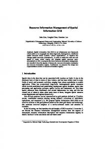
cover a wide range of the Pig features and operators, and the data set are generated with similar properties to Yahoo’s datasets that are commonly processed using Pig. With the exception of L11 (that contains a stage with 2 concurrent jobs), all PigMix programs involve DAGs of sequential jobs. Therefore, with the PigMix benchmark we mostly evaluate the accuracy of the proposed performance model for completion time estimates and resource allocation decisions,. The efficiency of the designed optimization technique for concurrent job execution is evaluated with the next two workloads in the set. TPC-H. This workload is based on TPC-H [1], a standard database benchmark for decision-support workloads. We select three queries Q5, Q8, Q10 out of existing 22 SQL queries and express them as Pig programs. For each query, we select a logical plan that results in a DAG of concurrent MapReduce jobs shown in Fig. 6 (a),(b),(c) respectively4 :
2. An experimental dataset: It is used to validate our performance models using the profiles extracted from the Pig programs that were executed with the test dataset. Both the test and experimental datasets are formed by the tables with the same layout but with different input sizes. • For PigMix benchmark, the input size of the experimental dataset is 20% larger than the test dataset (with 150 million records for the largest table). • For TPC-H, the experimental dataset is around 15 GB (scaling factor 15 using the standard data generator). • For HP Labs’ Web proxy query set, we use the logs from May, June and July as the experimental dataset, the total input size is around 9 GB.
• The TPC-H Q5 query joins 6 tables, and its dataflow results in 3 concurrent MapReduce jobs. • The TPC-H Q8 query joins 8 tables, and its dataflow results in two stages with 4 and 2 concurrent jobs. • The TPC-H Q10 query joins 4 tables, and its dataflow results in 2 concurrent MapReduce jobs. HP Labs’ Web Proxy Query Set. This workload consists of a set of Pig programs for analyzing HP Labs’ web proxy logs. It contains 6 months access logs to web proxy gateway at HP Labs. The fields include information such as date, time, time-taken, c-ip, cs-host, etc. We intend to create realistic Pig queries executed on real-world data. • The Proxy Q1 program investigates the dynamics in access frequencies to different websites per month and compares them across different months. The Pig program results in 3 concurrent MapReduce jobs with the DAG of the program shown in Figure 6 (d). • The Proxy Q2 program discovers the co-relationship between two websites from different sets (tables) of popular websites: the first set is created to represent the top 500 popular websites accessed by web users within the enterprise. The second set contains the top 100 popular websites in US according to Alexa’s statistics5 . The program DAG is shown in Figure 6 (e). • The Proxy Q3 program presents the intersection of 100 most popular websites (i.e., websites with highest access frequencies) accessed both during work and after work hours. The DAG of the program is shown in Figure 6 (f). To perform the validation experiments, we create two different datasets for each of the three workloads above: 4
While more efficient logical plans may exist, our goal here is to create a DAG with concurrent jobs to stress test our model. 5 http://www.alexa.com/topsites
5.
PERFORMANCE EVALUATION
This section presents the performance evaluation of the proposed models and optimizations. Since PigMix benchmark mostly consists of the Pig programs with sequential DAGs, we use PigMix only for validating the accuracy of the proposed performance models. Because TPC-H and HP Labs’ proxy log queries represent Pig programs that are defined by the DAGs with concurrent jobs, we use these two workloads for evaluating the performance benefits of introduced Pig program optimization as well as the models’ validation.
5.1
PigMix Case Study
This section aims to evaluate the accuracy of the proposed models: i) the bound-based model for estimating the completion time of Pig programs as a function of allocated resources, and ii) the accuracy of the recommended resource allocation for meeting the completion time goals. First, we run the Pigmix benchmark on the test dataset, and the job profiles of the corresponding Pig programs are built from these executions. By using the extracted job profiles and the designed Pig model we compute the completion time estimates of Pig programs in the PigMix benchmark for processing these two datasets (test and experimental) as a function of allocated resources. Then we validate the predicted completion times against the measured ones.
2
1.5
low Tavg T up T Measured-CT
1
0.5
0
L1 L2 L3 L4 L5 L6 L7 L8 L9 L10 L11 L12 L13 L14 L15 L16 L17
Figure 7: Predicted and measured completion time for PigMix executed with test dataset and 128x64 slots.
Program Completion Time
Figure 8 shows the results for the PigMix benchmark that processes the test dataset with 64 map and 64 reduce slots. Indeed, our model accurately computes the program completion time estimates as a function of allocated resources: the actual completion times of all 17 programs are between the computed lower and upper bounds. The predicted completion times based on the average of the upper and lower bounds provide the best results: 10-12% of the measured results for most cases. 2
1.5
Tlow Tavg Tup Measured-CT
1
L1 L2 L3 L4 L5 L6 L7 L8 L9 L10 L11 L12 L13 L14 L15 L16 L17
Figure 8: Predicted and measured completion time for PigMix executed with test dataset and 64x64 slots.
Program Completion Time
Figure 9 shows the predicted vs measured completion times for the PigMix benchmark that processes the larger, experimental dataset with 64 map and 64 reduce slots. 2.5 2
low
T avg T Tup Measured-CT
1.5 1 0.5 0
1.8
low
T -based Tavg -based Tup-based Deadline
1.6 1.4 1.2 1 0.8 0.6 0.4 0.2 0
L1 L2 L3 L4 L5 L6 L7 L8 L9 L10 L11 L12 L13 L14 L15 L16 L17
Figure 10: PigMix executed with the experimental dataset: do we meet deadlines?
0.5
0
programs is between the low and upper bounds. The predicted completion times that are based on the average of the upper and lower bounds provide the best results: they are within 10% of the measured results for most cases. In Figures 7, 8, 9 we execute PigMix benchmark three times and report the measured completion time averaged across 3 runs. A variance for most programs in these three runs is within 1%-2%, with the largest variance being around 6%. Because the variance is so small, we have omitted the error bars in Figures 7, 8, 9. Our second set of experiments aims to evaluate the solution of the inverse problem: the accuracy of a resource allocation for a Pig program with a completion time goal, often defined as a part of Service Level Objectives (SLOs). In this set of experiments, let T denote the Pig program completion time when the program is processed with maximum available cluster resources (i.e., when the entire cluster is used for program processing). We set D = 3 · T as a completion time goal. Using the approach described in Section 3.4 we compute the required resource allocation, i.e., a tailored number of map and reduce slots that allow the Pig program to be completed with deadline D on a new experimental dataset. We compute resource allocations when D is targeted as either a lower bound, or upper bound or the average of lower and upper bounds on the completion time. Figure 10 shows the measured program completion times based on these three different resource allocations. Similar to our earlier results, for presentation purposes, we normalize the achieved completion times with respect to the given deadline D. Program Completion Time
Program Completion Time
Figure 7 shows the predicted vs measured results for the PigMix benchmark that processes the test dataset with 128 map and 64 reduce slots. Given that the completion times of different programs in PigMix are in a broad range of 100s – 2000s, for presentation purposes and easier comparison, we normalize the predicted completion times with respect to the measured ones. The three bars in Figure 7 represent the predicted completion times based on the lower (T low ) and upper (T up ) bounds, and the average of them (T avg ). We observe that the actual completion times (shown as the straight Measured-CT line) of all 17 programs fall between the lower and upper bound estimates. Moreover, the predicted completion times based on the average of the upper and lower bounds are within 10% of the measured results for most cases. The worst prediction (around 20% error) is for the Pig query L11.
L1 L2 L3 L4 L5 L6 L7 L8 L9 L10 L11 L12 L13 L14 L15 L16 L17
Figure 9: Predicted and measured completion time for PigMix executed with experimental dataset and 64x64 slots. As shown in Figure 9, our model and computed estimates are quite accurate. The measured completion time of all
In most cases, the resource allocation that targets D as a lower bound is insufficient for meeting the targeted deadline (e.g., the L10 program misses deadline by more than 20%). However, when we compute the resource allocation based on D as an upper bound – we are always able to meet the required deadline, but in most cases, we over-provision resources, e.g., L16 and L17 finish more than 20% earlier than a given deadline. The resource allocations based on the average between lower and upper bounds result in the closest completion time to the targeted program deadlines.
5.2
Optimal Schedule of Concurrent Jobs
Figure 11 shows the impact of concurrent jobs scheduling on the completion time of TPC-H and Proxy queries when each program is processed with 128 map and 64 reduce slots. Figures 11 (a) and (c) show two extreme measurements: the best program completion time (i.e., when the optimal schedule of concurrent jobs is chosen) and the worst one (i.e., when concurrent jobs are executed in the “worst” possible order based on our estimates). For presentation purposes, the best (optimal) completion time is normalized with respect to the worst one. The choice of optimal
0.6 0.4 0.2 0
Q5
Q8
Program Completion Time
1.4
Best-CT Worst-CT
1.2 1 0.8 0.6 0.4 0.2 0
Q1
Q2
1 0.8 0.6 0.4 0.2 0
Q10
(a) Job completion time
Q5
Q8
(b)
Stage tion time 1.4
Q10
comple-
1
0.6 0.4 0.2 0
Q1
Q2
Q3
Predicting Completion Time and Resource Allocation of Optimized Pig Programs
1
0.5
0
Q5
Q8
Q10
(a) TPC-H
Program Completion Time
Program Completion Time
Figure 12 shows the Pig program completion time estimates (we use TPavg in these experiments) based on the proposed performance model for TPC-H and Proxy queries with the experimental datasets. Figure 12 shows the results when each program is processed with 64x64 and 32x64 map and reduce slots respectively. CT-Predicted-64x64 CT-Predicted-32x64 Measured-CT
1
0.5
0
(a) Can we meet deadlines?
1.5
Proxy-Queries-RA TPC-H-RA Non-Optimized-RA
1
0.5
0
(b) Resource requirements
Figure 13: Resource allocations for optimized Pig programs executed with the experimental dataset.
grams. Therefore, the proposed optimal schedule of concurrent jobs leads to significant resource savings for deadlinedriven Pig programs.
(d)
schedule of concurrent jobs reduces the completion time by 10%-27% compared with the worse case ordering. Figures 11 (b) and (d) show completion times of stages with concurrent jobs under different schedules for the same TPC-H and Proxy queries. Performance benefits at the stage level are even higher: they range between 20%-30%.
1.5
Measured-Proxy-Queries Measured-TPC-H Deadline
0.8
Stage completion time Figure 11: Normalized completion time for different schedules of concurrent jobs: (a-b) TPC-H, (c-d) HP Labs proxy queries.
5.3
1.5
of optimized Pig programs. Best-CT Worst-CT
1.2
Q3
(c) Job completion time
Best-CT Worst-CT
1.2
Normalized Resource Requirements
0.8
Program Completion Time
1
1.4
Stage Completion Time
Best-CT Worst-CT
1.2
Stage Completion Time
Program Completion Time
1.4
1.5
CT-Predicted-64x64 CT-Predicted-32x64 Measured-CT
1
0.5
0
Q1
Q2
Q3
(b) Proxy’s Queries
Figure 12: Predicted Pig programs completion times executed with the experimental dataset.
In all cases, the predicted completion times are within 10% of the measured ones. Let T denote the Pig program completion time when program P is processed with maximum available cluster resources. We set D = 2 · T as a completion time goal (we use different deadlines for different experiments on purpose, in order to validate the accuracy of our models for a variety of parameters). Then we compute the required resource allocation for P executed with the experimental dataset to meet the deadline D. Figure 13 (a) shows measured completion times achieved by the TPC-H and Proxy’s queries respectively when they are assigned the resource allocations computed with the designed resource allocation model. All the queries complete within 10% of the targeted deadlines. Figure 13 (b) compares the amount of resources (the sum of map and reduce slots) for non-optimized and optimized executions of TPC-H and Proxy’s queries respectively. The optimized executions are able to achieve targeted deadlines with much smaller resource allocations (20%-40% smaller) compared to resource allocations for non-optimized Pig pro-
6.
RELATED WORK
While performance modeling in the MapReduce framework is a new topic, there are several interesting research efforts in this direction. Polo et al. [14] introduce an online job completion time estimator which can be used in their new Hadoop scheduler for adjusting the resource allocations of different jobs. However, their estimator tracks the progress of the map stage alone, and use a simplistic way for predicting the job completion time, while skipping the shuffle/sort phase, and have no information or control over the reduce stage. FLEX [19] develops a novel Hadoop scheduler by proposing a special slot allocation schema that aims to optimize some given scheduling metric. FLEX relies on the speedup function of the job (for map and reduce stages) that defines the job execution time as a function of allocated slots. However, it is not clear how to derive this function for different applications and for different sizes of input datasets. The authors do not provide a detailed MapReduce performance model for jobs with targeted job deadlines. ARIA [17] introduces a deadline-based scheduler for Hadoop. This scheduler extracts the job profiles from the past executions, and provides a variety of bounds-based models for predicting a job completion time as a function of allocated resources and a solution of the inverse problem. However, these models apply only to a single MapReduce job. Tian and Chen [16] aim to predict performance of a single MapReduce program from the test runs with a smaller number of nodes. They consider MapReduce processing at a fine granularity. For example, the map task is partitioned in 4 functions: read a block, map function processing of the block, partition and sort of the processed data, and the combiner step (if it is used). The reduce task is decomposed in 4 functions as well. The authors use a linear regression technique to approximate the cost (duration) of each function. These functions are used for predicting the larger dataset processing. There are a few simplifying assumptions, e.g., a single wave in the reduce stage. The problem of finding resource allocations that support given job completion goals are formulated as an optimization problem that can be solved with existing commercial solvers. There is an interesting group of papers that design a detailed job profiling approach for pursuing a different goal: to optimize the configuration parameters of both a Hadoop cluster and a given MapReduce job (or workflow of jobs) for achieving the improved completion time. Starfish project [8, 7] applies dynamic instrumentation to collect a detailed runtime monitoring information about job execution at a fine granularity: data reading, map processing, spilling, merging, shuffling, sorting, reduce processing and writing. Such a
detailed job profiling information enables the authors to analyze and predict job execution under different configuration parameters, and automatically derive an optimized configuration. One of the main challenges outlined by the authors is a design of an efficient searching strategy through the highdimensional space of parameter values. The authors offer a workflow-aware scheduler that correlate data (block) placement with task scheduling to optimize the workflow completion time. In our work, we propose complementary optimizations based on optimal scheduling of concurrent jobs within the DAG to minimize overall completion time. Kambatla et al [11] propose a different approach for optimizing the Hadoop configuration parameters (number of map and reduce slots per node) to improve MapReduce program performance. A signature-based (fingerprint-based) approach is used to predict the performance of a new MapReduce program using a set of already studied programs. The ideas presented in the paper are interesting but it is a position paper that does not provide enough details and lacking the extended evaluation of the approach. Ganapathi et al. [5] use Kernel Canonical Correlation Analysis to predict the performance of Hive queries. However, they do not attempt to model the actual execution of the MapReduce job: the authors discover the feature vectors through statistical correlation. CoScan [18] offers a special scheduling framework that merges the execution of Pig programs with common data inputs in such a way that this data is only scanned once. Authors augment Pig programs with a set of (deadline, reward) options to achieve. Then they formulate the schedule as an optimization problem and offer a heuristic solution. Morton et al. [12] propose ParaTimer: the progress estimator for parallel queries expressed as Pig scripts [6]. In their earlier work [13], they designed Parallax – a progress estimator that aims to predict the completion time of a limited class of Pig queries that translate into a sequence of MapReduce jobs. In both papers, instead of a detailed profiling technique that is designed in our work, the authors rely on earlier debug runs of the same query for estimating throughput of map and reduce stages on the input data samples provided by the user. The approach is based on precomputing the expected schedule of all the tasks, and therefore identifying all the pipelines (sequences of MapReduce jobs) in the query. The approach relies on a simplified assumption that map (reduce) tasks of the same job have the same duration. This work is closest to ours in pursuing the completion time estimates for Pig programs. However, the usage of the FIFO scheduler and simplifying assumptions limit the approach applicability for progress estimation of multiple jobs running in the cluster with a different Hadoop scheduler, especially if the amount of resources allocated to a job varies over time or differs from the debug runs that are used for measurements.
7.
mated SLO-driven resource sizing and provisioning of complex workflows defined by the DAGs of MapReduce jobs. Moreover, our approach offers an optimized scheduling of concurrent jobs within a DAG that allows to significantly reduce the overall completion time. Our performance models are designed for the case without node failures. We see a natural extension for incorporating different failure scenarios and estimating their impact on the application performance and achievable “degraded” SLOs. We intend to apply designed models for solving a broad set of problems related to capacity planning of MapReduce applications (defined by the DAGs of MapReduce jobs) and the analysis of various resource allocation trade-offs for supporting their SLOs.
8.[1] TPC REFERENCES Benchmark H (Decision Support), Version 2.8.0, [2] [3]
[4]
[5]
[6]
[7]
[8]
[9]
[10]
[11]
[12]
[13]
[14]
[15]
CONCLUSION
Design of new job profiling tools and performance models for MapReduce environments has been an active research topic in industry and academia during past few years. Most of these efforts were driven by design of new schedulers to satisfy the job specific goals and to improve cluster resource management. In our work, we have introduced a novel performance modeling framework for processing Pig programs with deadlines. Our job profiling technique is not intrusive, it does not require any modifications or instrumentation of either the application or the underlying Hadoop/Pig execution engines. The proposed approach enables auto-
[16]
[17]
[18]
[19]
Transaction Processing Performance Council (TPC), http://www.tpc.org/tpch/, 2008. Apache. PigMix Benchmark, http://wiki.apache.org/pig/PigMix, 2010. R. Chaiken, B. Jenkins, P.-A. Larson, B. Ramsey, D. Shakib, S. Weaver, and J. Zhou. Easy and Efficient Parallel Processing of Massive Data Sets. Proc. of the VLDB Endowment, 1(2), 2008. J. Dean and S. Ghemawat. MapReduce: Simplified Data Processing on Large Clusters. Communications of the ACM, 51(1), 2008. A. Ganapathi, Y. Chen, A. Fox, R. Katz, and D. Patterson. Statistics-driven workload modeling for the cloud. In Proc. of 5th International Workshop on Self Managing Database Systems (SMDB), 2010. A. Gates, O. Natkovich, S. Chopra, P. Kamath, S. Narayanam, C. Olston, B. Reed, S. Srinivasan, and U. Srivastava. Building a High-Level Dataflow System on Top of Map-Reduce: The Pig Experience. Proc. of the VLDB Endowment, 2(2), 2009. H. Herodotou and S. Babu. Profiling, What-if Analysis, and Costbased Optimization of MapReduce Programs. In Proc. of the VLDB Endowment, Vol. 4, No. 11, 2011. H. Herodotou, H. Lim, G. Luo, N. Borisov, L. Dong, F. Cetin, and S. Babu. Starfish: A Self-tuning System for Big Data Analytics. In Proc. of 5th Conf. on Innovative Data Systems Research (CIDR), 2011. M. Isard, M. Budiu, Y. Yu, A. Birrell, and D. Fetterly. Dryad: Distributed Data-Parallel Programs from Sequential Building Blocks. ACM SIGOPS OS Review, 41(3), 2007. S. Johnson. Optimal Two- and Three-Stage Production Schedules with Setup Times Included. Naval Res. Log. Quart., 1954. K. Kambatla, A. Pathak, and H. Pucha. Towards optimizing hadoop provisioning in the cloud. In Proc. of the First Workshop on Hot Topics in Cloud Computing, 2009. K. Morton, M. Balazinska, and D. Grossman. ParaTimer: a progress indicator for MapReduce DAGs. In Proc. of SIGMOD. ACM, 2010. K. Morton, A. Friesen, M. Balazinska, and D. Grossman. Estimating the progress of MapReduce pipelines. In Proc. of ICDE, 2010. J. Polo, D. Carrera, Y. Becerra, J. Torres, E. Ayguad´ e, M. Steinder, and I. Whalley. Performance-Driven Task Co-Scheduling for MapReduce Environments. In Proc. of the 12th IEEE/IFIP Network Operations and Management Symposium, 2010. A. Thusoo, J. S. Sarma, N. Jain, Z. Shao, P. Chakka, S. Anthony, H. Liu, P. Wyckoff, and R. Murthy. Hive - a Warehousing Solution over a Map-Reduce Framework. Proc. of VLDB, 2009. F. Tian and K. Chen. Towards Optimal Resource Provisioning for Running MapReduce Programs in Public Clouds. In Proc. of IEEE Conference on Cloud Computing (CLOUD 2011). A. Verma, L. Cherkasova, and R. H. Campbell. ARIA: Automatic Resource Inference and Allocation for MapReduce Environments. Proc. of the 8th ACM International Conference on Autonomic Computing (ICAC’2011), 2011. X. Wang, C. Olston, A. Sarma, and R. Burns. CoScan: Cooperative Scan Sharing in the Cloud. In Proc. of the ACM Symposium on Cloud Computing,(SOCC’2011), 2011. J. Wolf, D. Rajan, K. Hildrum, R. Khandekar, V. Kumar, S. Parekh, K.-L. Wu, and A. Balmin. FLEX: A Slot Allocation Scheduling Optimizer for MapReduce Workloads. Proc. of the 11th ACM/IFIP/USENIX Middleware Conference, 2010.