Oct 21, 2015 - Automated Synchronization of Driving Data. Using Vibration and Steering Events. Lex Fridman1, Daniel E. Brown1, William Angell1, Irman ...
Automated Synchronization of Driving Data Using Vibration and Steering Events Lex Fridman1 , Daniel E. Brown1 , William Angell1 , Irman Abdi´c1 , Bryan Reimer1 , and Hae Young Noh2
arXiv:1510.06113v1 [cs.RO] 21 Oct 2015
1
Massachusetts Institute of Technology (MIT) 2 Carnegie Mellon University (CMU)
Abstract—We propose a method for automated synchronization of vehicle sensors useful for the study of multi-modal driver behavior and for the design of advanced driver assistance systems. Multi-sensor decision fusion relies on synchronized data streams in (1) the offline supervised learning context and (2) the online prediction context. In practice, such data streams are often out of sync due to the absence of a real-time clock, use of multiple recording devices, or improper thread scheduling and data buffer management. Cross-correlation of accelerometer, telemetry, audio, and dense optical flow from three video sensors is used to achieve an average synchronization error of 13 milliseconds. The insight underlying the effectiveness of the proposed approach is that the described sensors capture overlapping aspects of vehicle vibrations and vehicle steering allowing the cross-correlation function to serve as a way to compute the delay shift in each sensor. Furthermore, we show the decrease in synchronization error as a function of the duration of the data stream. Index Terms—Passive synchronization; cross correlation; vehicle sensor fusion; optical flow; on-road driving data.
I. I NTRODUCTION Large multi-sensor on-road driving datasets offer the promise of helping researchers develop a better understanding of driver behavior in the real world and aid in the design of future advanced driver assistance systems (ADAS) [1], [2]. As an example, the Strategic Highway Research Program (SHRPR 2) Naturalistic Driving Study includes over 3,400 drivers and vehicles with over 5,400,000 trip records [3] that contains video, telemetry, accelerometer, and other sensor data. The most interesting insights are likely to be discovered not in the individual sensor streams but in their fusion. However, sensor fusion requires accurate sensor synchronization. The practical challenge of fusing “big data”, especially in the driving domain, is that it is often poorly synchronized, especially when individual sensor streams are collected on separate hardware [4]. A synchronization error of 1 second may be deemed acceptable for traditional statistical analyses that focus on data aggregated over a multi-second or multi-minute windows. But in the driving context, given high speed and close proximity to surrounding vehicles, a lot can happen in less than one second. We believe that the study of behavior in relation to situationally relevant cues and the design of an ADAS system that supports driver attention on a moment-to-moment basis requires a maximum synchronization error of 100 milliseconds. For example, events associated with glances (e.g.,
eye saccades, blinks) often occur on a sub-100-millisecond timescale [5]. Hundreds of papers are written every year looking at the correlation between two or more aspects of driving (e.g., eye movement and steering behavior). The assumption in many of these analyses is that the underlying data streams are synchronized or aggregated over a long enough window that the synchronization error is not significantly impacting the interpretation of the data. Often, these assumptions are not thoroughly tested. The goal of our work is to motivate the feasibility and the importance of automated synchronization of multi-sensor driving datasets. We propose two event types (vehicle vibration and vehicle steering), that can be detected by video, audio, telemetry, and accelerometer sensors. Crosscorrelation of processed sensor streams is used to compute the time-delay of each sensor pair. We evaluate the automated synchronization framework on a small dataset and achieve an average synchronization error of 13 milliseconds. We also characterize the increase in accuracy with respect to increasing data stream duration which motivates the applicability of this method to online synchronization. The implementation tutorial and source code for this work will be made available at: http://lexfridman.com/carsync II. R ELATED W ORK Sensor synchronization has been studied thoroughly in the domain of sensor networks where, generally, a large number of sensor nodes are densely deployed over a geographic region to observe specific events [6], [7]. The solution is in designing robust synchronization protocols to provide a common notion of time to all the nodes in the sensor network [8]. These protocols rely on the ability to propagate ground truth timing information in a master-slave or peer-to-peer framework. Our paper proposes a method for inferring this timing information from the data itself, in a passive way as in [9]. This is only possible when the sensors are observing largely-overlapping events. Our paper shows that up-down vibrations and leftright turns serve as discriminating events in the driving context around which passive sensor synchronization can be performed. The main advantage of passive synchronization is that it
requires no extra human or hardware input outside of the data collection itself. As long as the sensors observe overlapping aspects of events in the external environment, the data stream itself is all that is needed. The challenge of passive synchronization is that sensors capture non-overlapping aspects of the environment as well. The overlapping aspects are the “signal” and the non-overlapping aspects are the “noise”. Given this definition of signal and noise, the design of an effective passive synchronization system requires the use of sensor pairs with low signal-to-noise ratio. Despite its importance, very little work has been done on passive synchronization of sensors, especially in the driving domain. This general problem was addressed in [10] using an interval-based method for odometry and video sensors on mobile robots. Their approach uses semi-automated and sparse event extraction. The event-extraction in this paper is densely sampled and fully automated allowing for higher synchronization precision and greater robustness to noisy event measurements. The pre-processing of video data for meaningful synchronizing event extraction was performed in [11] for gesture recognition. We apply this idea to video data in the driving context using dense optical flow. Optical flow has been used in the driving domain for object detection [12] and image stabilization [13]. Since then, dense optical flow has been successfully used for ego-motion estimation [14]. We use the ability of optical flow to capture fast ego-motion (i.e., vibration) for the front camera and scene vibration for the face and dash cameras in order to synchronize video data with accelerometer data. Flow-based estimation of ego-rotation is used to synchronize front video and steering wheel position.
2) We clapped three times at the beginning and the end of the each run. This was done in front of the camera such that the tire microphone could pick up the sound of each clap. This allowed us to manually synchronize the audio and the video. 3) We visualized the steering wheel (see Fig. 2) according to the steering wheel position reported in the CAN and lined it up to the steering wheel position in the video of the dashboard. This allows us to manually synchronize video and telemetry. A real-time clock module was used to assign timestamps to all discrete samples of sensor data. This timestamp and the above three manual synchronization methods were used to produce the ground truth dataset over which the evaluation in §IV is performed. A. Sensors The following separate sensor streams are collected and synchronized in this work: •
Front Video Camera: 720p 30fps video of the forward roadway. Most of the optical flow motion in the video is of the external environment. Therefore, vibration is captured through ego-motion estimated by the vertical component of the optical flow. Steering events are captured through the horizontal component of the optical flow. See §III-B.
•
Dash Video Camera: 720p 30fps video of the dashboard. This is the most static of the video streams, so spatiallyaveraged optical flow provides the most accurate estimate of vibrations.
•
Face Video Camera: 720p 30fps video of the driver’s face. This video stream is similar to dashboard video except for the movements of the driver. These movements contribute noise to the optical flow vibration estimate.
•
Inertial Measurement Unit (IMU): Accelerometer used to capture the up-down vibrations of the vehicle that correspond to y-axis vibrations in the video. Average sample rate is 48 Hz.
•
Audio: Shotgun microphone attached behind the right rear tire of the vehicle used to capture the interaction of the tire with the surface. Sample rate is 44,100 Hz and bit depth is 16.
•
Vehicle Telemetry: Parsed messages from the controller area network (CAN) vehicle bus reduced down in this work to just steering wheel position. Sample rate is 100Hz.
III. DATASET AND S ENSORS In order to validate the proposed synchronization approach we instrumented a 2014 Mercedes CLA with a single-board computer and consumer-level inexpensive sensors: 3 webcams, a shotgun microphone behind the rear tire, GPS, an IMU module, and a CAN controller for vehicle telemetry. The instrumented vehicle is shown in Fig. 1. The collection of data was performed on 5 runs, each time traveling the same route in different traffic conditions. The duration of each run spanned from 37 minutes to 68 minutes. Unless otherwise noted, the illustrative figures in this paper are based on the 37 minute run. Three manual synchronization techniques were used on each run to ensure that perfect synchronization was achieved and thus can serve as the ground truth for the proposed automated synchronization framework: 1) The same millisecond-resolution clock was placed in front of each camera at the beginning and end of each run. This allowed us to manually synchronize the videos together.
A snapshot from a video visualization of these sensor streams is shown in Fig. 2. GPS position was collected but not used as part of the synchronization because its average sample rate
Instrumented Vehicle
Face Camera
Data Collection Device Shotgun Microphone
Dashboard Camera
Front Camera
Fig. 1: The instrumented vehicle, cameras, and single-board computer used for collecting the data to validate the proposed synchronization approach.
Front Video
Observation of Steering Events
Dash Video
Observation of Vibrations Events
Face Video
Front Flow Accelerometer
GPS Location
Face Flow
Wheel
Dash Flow
Front Flow
Audio Energy
Dense Optical Flow of Front Video
Fig. 2: Snapshot from a 30 fps video visualization of a synchronized set of sensors collected for the 37 minute experimental run used throughout the paper as an example. Full video available online at: http://lexfridman.com/carsyncvideo
is 1 Hz which is 1 to 2 orders of magnitude less frequent than the other sensors.
The optimal time shift δ ∗ for synchronizing the two data streams is computed by choosing the t that maximizes the cross correlation function:
B. Dense Optical Flow The dense optical flow is computed as a function of two images taken at times t and t+∆t, where ∆t varies according to the frame rate of the video (30 fps in the case of this paper) and the burstiness of frames due to the video buffer size. We use the Farneback algorithm [15] to compute the dense optical flow. It estimates the displacement field using a quadratic polynomial for the neighborhood of each pixel. The algorithm assumes a slowly varying displacement field, which is a valid assumption for the application of detecting vibrations and steering since those are events which affect the whole image uniformly relative to the depth of the object in the image. Segmentation was used to remove non-static objects, but it did not significantly affect the total magnitude of either the x or y components of the flow. The resulting algorithm produces a flow for which the following holds: I(x, y, t) = I(x + ∆x, y + ∆y, t + ∆t)
(1)
where I(x, y, t) is the intensity of the pixel (x, y) at time t, ∆x is the x (horizontal) component of the flow, and ∆y is the y (vertical) component of the flow. These two components are used separately as part of the synchronization. The vertical component is used to measure the vibration of the vehicle and the horizontal component is used to measure the turning of the vehicle. IV. S YNCHRONIZATION F RAMEWORK Unless otherwise noted, the figures in this section show sensor traces and cross correlation functions for a single 37 minute example run. The two synchronizing event types are vibrations and steering, both densely represented throughout a typical driving session. A. Cross-Correlation Cross-correlation has long been used as a way to estimate time delay between two regularly sampled signals [16]. We use an efficient FFT-based approach for computing the cross correlation function [17] with an O(n log n) running time complexity (compared to O(n2 ) running time of the naive implementation): def
(f ? g)[t] =
∞ X
f [i] g[i + t]
(2)
δ ∗ = arg max(f ? g)[t]
(3)
t
This optimization assumes that the optimal shift corresponds to maximum positive correlation. Three of the sensors under consideration are negatively correlated: (1) vertical component of face video optical flow, (2) vertical component of dash video optical flow, and (3) horizontal component of front video optical flow. These three were multiplied by -1, so that all sensors used for synchronization are positively correlated. Vibration and steering events are present in all vehicle sensors, but post processing is required to articulate these events in the data. Accelerometer and steering wheel position require no post-processing for the cross correlation computation in (3). The three video streams were processed to extract horizontal and vertical components of dense optical flow as discussed in §III-B. The shotgun microphone audio was processed by summing the audio energy in each 10 ms increment. Several filtering methods (Wiener filter, total variation denoising, and stationary wavelet transform) under various parameter settings were explored programmatically, but they did not improve the optimal time shift computation accuracy as compared to cross correlation of un-filtered sensor data. Fig. 3 shows the sensor trace and cross correlation functions for the z component of acceleration, the y component of dense optical flow for the three videos, and discretized audio energy. These data streams measure the vibration of the vehicle during the driving session. All of them capture major road bumps and potholes. The audio captures more complex properties of the surface which makes vibration-based synchronization with audio the most noisy of the five sensors. These 5 sensors can be paired in 10 ways. We found that the most robust and least noisy cross correlation function optimization was for the pairing all sensors with the accelerometer. This is intuitive since the accelerometer is best able to capture vibration. The resulting 4 cross correlation functions for the 37 minute example run are shown in Fig. 3b. Fig. 4 shows the sensor trace and cross correlation function for the x component of dense optical flow for the front video and the position of the steering wheel. This is an intuitive pairing of sensors that produced accurate results for our experiments in a single vehicle. However, since the way a vehicle’s movement corresponds to steering wheel position depends on the sensitivity of the steering wheel, the normalizing sensorpair delay (see §IV-B) may vary from vehicle to vehicle.
i=−∞
B. Online and Offline Synchronization where f and g are real-valued discrete functions, t is the time shift of g, and both f and g are zero for i and i + t outside the domain of f and g respectively.
Table I shows the results of computing the optimal delay δ ∗ for each sensor pairing in each of the 5 runs as discussed
Accelerometer (Z)
Front Flow (Y)
Tire Audio
0.5 1.0 1.5 2.0 3 2 1 0 1 2 10 5 0
Dash Flow (Y)
0
Face Flow (Y)
10
3 2 1 0 1 2 0
5 5
5
10
15
20
Time (mins)
25
30
35
(a) The accelerometer, video, and audio sensors capturing the vibration of the vehicle. The x-axis is time in minutes and the y-axis is the value of the sensor reading.
Accelerometer (Z) / Tire Audio δ ∗ = -320.0 ms
Accelerometer (Z) / Front Flow (Y) δ ∗ = -280.0 ms
Accelerometer (Z) / Dash Flow (Y) δ ∗ = 240.0 ms
Accelerometer (Z) / Face Flow (Y) δ ∗ = 90.0 ms
(b) The cross-correlation functions and optimal time-delay δ ∗ of audio and video with respect to the accelerometer. The x-axis is the shift t in (2) and the y-axis is the magnitude of the correlation.
Fig. 3: The vibration-based synchronization for the 37-minute example run.
Front Flow (X) Steering Wheel
400 300 200 100 0 100 200 300 400 10 5 0 5 10 15 20 0
TABLE I: The mean and standard deviation of the optimal delay δ ∗ in (3). The mean serves as the normalizing sensorpair delay. The standard deviation, in this case, is an estimate for average synchronization error. Across the five sensor pairs listed here, the average error is 13.5 ms.
5
10
15
20
Time (mins)
25
30
35
(a) The telemetry and video sensors capturing the steering of the vehicle. The x-axis is time in minutes and the y-axis is the value of the sensor reading.
Steering Wheel / Front Flow (X) δ ∗ = 310.0 ms
(b) The cross-correlation functions and optimal time-delay δ ∗ of telemetry and front video. The x-axis is the shift t in (2) and the y-axis is the magnitude of the correlation.
Fig. 4: The steering-based synchronization for the 37-minute example run.
Synchronization Error (ms)
250 200 150 100 50 0 5
10
15
20
25
30
Time Into Data Recording (mins)
35
40
Fig. 5: The decrease of synchronization error versus the duration of the data stream. The mean and standard deviation forming the points and errorbars in the plot are computed over 5 sensor pairs and over 5 runs, each of which involved the instrumented vehicle traveling same route (lasting 37-68 minutes).
Sensor Pair
avg(δ ∗ ) (ms)
std(δ ∗ ) (ms)
Accelerometer / Tire Audio
305.2
22.8
Accelerometer / Front Flow
-279.9
12.7
Accelerometer / Dash Flow
246.4
8.7
Accelerometer / Face Flow
95.0
14.2
Steering Wheel / Front Flow
312.1
9.3
in §IV-A. The value avg(δ ∗ )for each sensor pairing is the “normalizing delay”, which is an estimate of the delay inherent in the fact that optical flow, audio energy, accelerometer, and steering wheel position are capturing different temporal characteristics of the same events. For example, there is a consistent delay of just over 300ms between steering wheel position and horizontal optical flow in the front camera. This normalizing delay is to be subtracted from δ ∗ computed on future data in order to determine the best time shift for synchronizing the pair of sensor streams. In this case, the standard deviation std(δ ∗ )is an estimate of the synchronization error. For the 5 runs in our dataset, the average error is 13.5 ms which satisfies the goal of sub-100 ms accuracy stated in §I. The proposed synchronization framework is designed as an offline system for post-processing sensor data after the data collection has stopped. However, we also consider the tradeoff between data stream duration and synchronization accuracy in order to evaluate the feasibility of this kind of passive synchronization to be used in an online real-time system. Fig. 5 shows the decrease in synchronization error versus the duration of the data stream. Each point averages 5 sensor pairings over 5 runs. While the duration of each run ranged from 37 to 68 minutes, for this plot we only average over the first 37 minutes of each run. The synchronization error here is a measurement of the difference between the current estimate of δ ∗ and the one converged to after the full sample is considered. This error does not consider the ground truth which is estimated to be within 13.5 ms of this value. Data streams of duration less than 8 minutes produced synchronization errors 1-2 orders of magnitude higher than the ones in this plot. The takeaway from this tradeoff plot is that an online system requires 10 minutes of data to synchronize the multi-sensor stream to a degree that allows it to make real-time decisions based on the fusion of these sensors. V. C ONCLUSION Analysis and prediction based on fusion of multi-sensor driving data requires that the data is synchronized. We propose
a method for automated synchronization of vehicle sensors based on vibration and steering events. This approach is applicable in both an offline context (i.e., for driver behavior analysis) and an online context (i.e., for real-time intelligent driver assistance). We show that a synchronization error of 13.5 ms can be achieved for a driving session of 35 minutes. ACKNOWLEDGMENT Support for this work was provided by the New England University Transportation Center, and the Toyota Class Action Settlement Safety Research and Education Program. The views and conclusions being expressed are those of the authors, and have not been sponsored, approved, or endorsed by Toyota or plaintiffs class counsel. R EFERENCES [1] L. Fridman and B. Reimer, “Semi-automated annotation of discrete states in large video datasets,” in AAAI, 2016, p. Submitted. [2] B. Reimer, “Driver assistance systems and the transition to automated vehicles: A path to increase older adult safety and mobility?” Public Policy & Aging Report, vol. 24, no. 1, pp. 27–31, 2014. [3] J. F. Antin, Design of the in-vehicle driving behavior and crash risk study: in support of the SHRP 2 naturalistic driving study. Transportation Research Board, 2011. [4] W. Q. Meeker and Y. Hong, “Reliability meets big data: Opportunities and challenges,” Quality Engineering, vol. 26, no. 1, pp. 102–116, 2014. [5] D. K. McGregor and J. A. Stern, “Time on task and blink effects on saccade duration,” Ergonomics, vol. 39, no. 4, pp. 649–660, 1996. [6] F. Sivrikaya and B. Yener, “Time synchronization in sensor networks: a survey,” Network, IEEE, vol. 18, no. 4, pp. 45–50, 2004. [7] I.-K. Rhee, J. Lee, J. Kim, E. Serpedin, and Y.-C. Wu, “Clock synchronization in wireless sensor networks: An overview,” Sensors, vol. 9, no. 1, pp. 56–85, 2009. [8] J. Elson, L. Girod, and D. Estrin, “Fine-grained network time synchronization using reference broadcasts,” ACM SIGOPS Operating Systems Review, vol. 36, no. SI, pp. 147–163, 2002. [9] E. Olson, “A passive solution to the sensor synchronization problem,” in Intelligent Robots and Systems (IROS), 2010 IEEE/RSJ International Conference on. IEEE, 2010, pp. 1059–1064. [10] M. Zaman and J. Illingworth, “Interval-based time synchronisation of sensor data in a mobile robot,” in Intelligent Sensors, Sensor Networks and Information Processing Conference, 2004. Proceedings of the 2004. IEEE, 2004, pp. 463–468. [11] T. Pl¨otz, C. Chen, N. Y. Hammerla, and G. D. Abowd, “Automatic synchronization of wearable sensors and video-cameras for ground truth annotation–a practical approach,” in Wearable Computers (ISWC), 2012 16th International Symposium on. IEEE, 2012, pp. 100–103. [12] P. H. Batavia, D. Pomerleau, C. E. Thorpe et al., “Overtaking vehicle detection using implicit optical flow,” in Intelligent Transportation System, 1997. ITSC’97., IEEE Conference on. IEEE, 1997, pp. 729– 734. [13] A. Giachetti, M. Campani, and V. Torre, “The use of optical flow for road navigation,” Robotics and Automation, IEEE Transactions on, vol. 14, no. 1, pp. 34–48, 1998. [14] V. Grabe, H. H. B¨ulthoff, D. Scaramuzza, and P. R. Giordano, “Nonlinear ego-motion estimation from optical flow for online control of a quadrotor uav,” The International Journal of Robotics Research, p. 0278364915578646, 2015.
[15] G. Farneb¨ack, “Two-frame motion estimation based on polynomial expansion,” in Image Analysis. Springer, 2003, pp. 363–370. [16] C. H. Knapp and G. C. Carter, “The generalized correlation method for estimation of time delay,” Acoustics, Speech and Signal Processing, IEEE Transactions on, vol. 24, no. 4, pp. 320–327, 1976. [17] J. Lewis, “Fast normalized cross-correlation,” in Vision interface, vol. 10, no. 1, 1995, pp. 120–123.