Boundary integral equation, Laplace's equation, numerical integral equation, com- puter program ... The NAG library 8] contains a routine D03EAF for using.
AUTOMATIC BOUNDARY INTEGRAL EQUATION PROGRAMS FOR THE PLANAR LAPLACE EQUATION KENDALL ATKINSON� AND YOUNGMOK JEONy
Abstract. Algorithms with automatic error control are described for the solution of Laplace's equation on both interior and exterior regions, with both Dirichlet and Neumann boundary conditions. The algorithms are based on standard reformulations of each boundary value problem as a boundary integral equation of the second kind. The Nystrom method is used to solve the integral equations, and convergence of arbitrary high order is observed when the boundary data is analytic. The Kelvin transformation is introduced to allow a simple conversion between internal and external problems. Two Fortran program implementations, DRCHLT and NEUMAN, are de ned, analyzed, and illustrated. Key words.
puter program
Boundary integral equation, Laplace's equation, numerical integral equation, com-
AMS subject classi cation. Primary: 65N38; Secondary 65R20, 45L10
1. Introduction. This paper presents two programs with automatic error control
for solving Laplace's equation in two dimensions. The programs are based on solving standard boundary integral equation (BIE) reformulations of various boundary value problems. Let denote a bounded simply connected planar region with a smooth boundary ?. The programs treat both the Dirichlet and Neumann problems, for both interior and exterior regions, for such regions . We use standard BIE reformulations of Laplace's equation, and the numerical methods are also quite standard. The programs are of interest in that they are automatic in selecting various problem parameters so as to ensure a requested error tolerance. Moreover, we believe the programs are robust and relatively e�cient, especially when the requested error tolerances are small or when the region is not convex and has a complicated boundary. The NAG library [8] contains a routine D03EAF for using boundary integral representations to solve Laplace's equation. That program requires the user to specify the discretization parameter, and it does not contain any means to estimate the error in the computed solution, in contrast to our codes. For that reason, we have not included any numerical comparisons with D03EAF. Our codes, however, are restricted to smooth boundaries ?, which is not a restriction with the NAG routine. In x2, we review the reformulation of the interior Dirichlet problem and the exterior Neumann problems as boundary integral equations; and we describe the numerical method used to solve these BIE. In x3, this work is extended to the exterior Dirichlet and interior Neumann problems, by means of applying a Kelvin transformation to convert the problems to those treated in x2. In x4, we describe the algorithms DRCHLT for the solution of the Dirichlet problem and NEUMAN for the Neumann problem. Numerical examples which explore the behaviour of the algorithms are given in x5. We note Dept of Mathematics, University of Iowa, Iowa City, IA 52242. This research is supported in part by NSF grant DMS-9403589 y Dept of Mathematics, A-Jou University, Su Won, Korea 441-749. The research is supported by Korean Ministry of Education under the grant number BSRI-96-1441. 1 �
particularly the numerical example for the \amoeba" boundary of Figure 2, as it is a region which would give a great deal of trouble to nite element and nite di�erence codes. 2. The Interior Dirichlet and Exterior Neumann Problems. The material of this and the following section is well-known, and the reader can nd an extensive development of it in [4, Chap. 7], Kress [5], or in a number of other texts on boundary integral equations. Consider rst the interior Dirichlet problem �u(A) = 0; A2
u(P ) = f (P ); P 2 ?
(1)
and assume that ? has a parameterization which is at least twice continuously di�erentiable. Represent u as a double layer potential Z (2) u(A) = ? �(Q) @n@ [log jA ? Qj] dSQ; A 2
Q ? in which nQ is the outward unit normal at Q 2 ?. Then � satis es the uniquely solvable integral equation Z ?��(P ) ? �(Q) @n@ [log jP ? Qj] dSQ = f (P ); P 2 ? (3) Q ? Parameterize ? by r(t) = (x(t); y(t)), 0 � t � 2�, where we assume jr0 (t)j 6= 0 for all t. Rewrite (3) as
(4)
?��(t) ?
Z 2�
0
�(s)K (t; s) ds = f (t); 0 � t � 2�
In this, we have identi ed �(r(t)) with �(t), for simplicity. For the kernel function, 8 > > >
00 0 y (t)x (t) ? x00 (t)y0(t) ; > > t=s : 2 [x0(t)2 + y0(t)2 ] With the assumption that r(t) is at least twice continuously di�erentiable, the kernel function K (t; s) is continuous; and for r 2 C q+2, it follows that K 2 C q with respect to all partial derivatives of K . We write (4) symbolically as (?� ? K) � = f The most e�cient way to solve (4) is to use the Nystrom method with the rectangle rule. This is because the integral in (4) is periodic in s with period 2�, and for such cases, the rectangle rule (or equivalently the trapezoidal rule, due to periodicity) is 2
a very rapidly convergent method. For example, if g belongs to the Sobolev space H [0; 2�] for some > 21 , and if g is periodic on [0; 2�], then (6)
Z 2� g(s) ds 0
?h
n X j =1
g (sj )
p
(2 ) � 4�� n kgkH ; n � 1
with h = 2�=n; sj = jh for j = 1; :::; n, and � (t) the Riemann Zeta function. The Nystrom approximation of (4) is given by (7)
?��n(t) ? h
n X j =1
K (t; sj )�n(sj ) = f (t); 0 � t � 2�
We write this symbolically as (?� ? Kn) �n = f with the numerical integral operator Kn de ned implicitly by (7). The equation (7) is equivalent in solvability to the linear system (8)
?��n (si) ? h
n X j =1
K (si; sj )�n(sj ) = f (si); i = 1; :::; n
The equivalence of these two formulas is given by the Nystrom interpolation formula "
(9)
#
n X �n(t) = ? �1 f (t) + h K (t; sj )�n(sj ) ; 0 � t � 2� j =1
enabling one to extend the solution f�n(si )g of (8) to �n(s) for general s. The equivalence is discussed in [4, p. 101]. We write (8) symbolically as (10)
(?� ? Kn) �n = fn;
� n ; fn 2 R n
By standard error analysis results (e.g. see [4, Chap. 4]), the operators ?� ? Kn are invertible for all su�ciently large n, say n � n0, and their inverses are uniformly bounded. Moreover, (11)
k� ? �nk1 � (?� ? Kn)?1 kK� ? Kn�k1 ; n � n0
Thus the smoother the curve and the smoother the data f , the faster the uniform convergence of �n to �. Precise bounds can be obtained from either (6) or the EulerMacLaurin formula (cf. [3, p. 285]). Using the latter, we have the following result. Let ? be (q + 2)-times di�erentiable, let � 2 C p(?), and let r = min fp; qg. Then
(12) k� ? �nk1 � ncr �(r) 1 3
for some c independent of n and r. By di�erentiating the equations (4) and (7) with respect to t, we can also obtain bounds on the rate of convergence of �(nk) to �(k) :
(k)
� ? �(k) � cr;k �(r) ; k = 1; :::; r ? 1 n 1 nr?k 1 for some cr;k independent of n. To solve approximately the Dirichlet problem (1), introduce the approximating potential Z un(A) = ? �n(Q) @n@ [log jA ? Qj] dSQ; A 2
(13) Q ? Using the parameterization of ?, rewrite this as (14)
un(A) = ? KA
Z 2�
0
(s) = jr0(s)j
�n (s)KA(s) ds; A 2
@ [log jA ? Qj] @nQ Q=r(s)
The function un is harmonic on . To look at the error u ? un, note rst that by the maximum principle, (15)
ju(A) ? un(A)j � max ju(P ) ? un(P )j P 2?
Let A ! P 2 ? in (13) and then subtract from (3) to obtain ?� [�(P ) ? �n(P )] ? R? [�(Q) ? �n(Q)] @n@ [log jP ? Qj] dSQ Q = u(P ) ? un(P ); P 2 ? Then max ju(P ) ? un(P )j � (� + kKk) k� ? �nk1 P 2? When combined with (15),
ju(A) ? un(A)j � (� + kKk) k� ? �nk1 ; A 2
If the region is convex, then kKk = � and the bound simpli es further. In the
(16)
program, we use the approximation
kKk = max t
Z 2�
0
n X : jK (si; sj )j jK (t; s)j ds = h 1max �i�n j =1
4
It is not di�cult to see that KA(s) is very peaked for A near to ?, with the maximum peaking occurring at the point of ? nearest to A. For that reason, we use a standard integral identity to write (17)
un(A) = ?2��n
(s�) ?
Z 2�
0
[�n(s) ? �n (s�)] KA(s) ds; A 2
with s� chosen to approximately minimize jr(s) ? Aj. This new integral is slightly better in terms of its behaviour for s near to s� . This is a standard technique, long used to reduce the e�ect of the peak in KA(s). To evaluate (17), we again use the rectangle rule, say with m nodes: (18)
m
X un;m(A) = ?2��n (s�) ? � [�n(�j ) ? �n (s�)] KA(�j ) j =1
with � = 2�=m, �j = j�, j = 1; 2; :::; m. In our program, we begin with n = n0 = 16, doubling as needed. The values of m begin with m = m0 = 32; and m is doubled as needed. When m exceeds n, the Nystrom formula (9) is used to extend �n to new argument values; and these are saved for possible use with other points A. The size of m is limited by the size of the workspace given to the subroutine DRCHLT. For the total error in un;m(A), (19)
ju(A) ? un;m(A)j � ju(A) ? un(A)j + jun(A) ? un;m(A)j � 0 � c c
(r) = nr (� + kKk) + �r mr � 1
In this, the bound on jun(A) ? un;m(A)j comes from [6], with
� = min jA ? P j P 2? The power of � in the denominator would be one greater if (13) had been used rather than (17). 2.1. The exterior Neumann problem. Consider the exterior Neumann problem �u(A) = 0; A 2 e @u(P ) = g(P ); P 2 ? (20) @nP u(A) ! 0 as jAj ! 1 in which e = R2 = . Again, nP is directed into e. Note that in the exterior Neumann problem, Z Z @u ( P ) (21) dSP = g(P )dSP = 0 u(A) ! 0 as jAj ! 1 , ? ? @nP 5
For details, see Kress [5]. Represent the solution u of (20) as a single layer potential,
u(A) = ?
(22)
Z
(Q) log jA ? Qj dSQ; A 2 e
?
By standard arguments, satis es the equation Z ?� (P ) ? (Q) @n@ [log jP ? Qj] dSQ = g(P ); P 2 ? (23) P ? Using the parameterization r(t) = (x(t); y(t)) for ?, (23) becomes
?� (t) ?
(24)
Z 2�
(s)Ke(t; s) ds = g(t); 0 � t � 2�
0
For the kernel function,
p
8 > > >
00 0 y (t)x (t) ? x00 (t)y0(t) ; > > : t=s 2 [x0(t)2 + y0(t)2 ] The integral equation (24) is solved in the same manner as earlier with the interior Dirichlet problem, resulting in an approximation n; and the error bounds and rates of convergence are also as before. For the approximation of u, introduce (25)
un(A) = ?
Z
n (Q) log jA ? Qj dSQ;
?
A 2 e
Using the parameterization of ?, we write (26)
un(A) = ?
Z 2�
0
n (s)Ke;A(s) ds;
A 2 e
Ke;A(s) = jr0(s)j log jA ? r(s)j Using the maximum principle and arguing as before, (27)
Z
ju(A) ? un(A)j � k ? nk1 sup jlog jP ? Qjj dSQ; A 2 e P 2? ?
We approximate un(A) by un;m(A), much as before in (18): (28)
un;m(A) = ?�
m X j =1
n (�j )Ke;A(�j );
6
A 2 e
The error bound for ju(A) ? un;m(A)j is exactly the same as that in (19) for the approximation of the double layer potential, with � replace by and with other choices for c and c0. For the case that P 2 ?, we must use an alternative to (28). Rewrite (26) as
un(r(t)) = �A en(t) ? R en (t);
(29) In this, we write
jr j
en (t) = n (t) 0 (t) , Z 2�
A'(t) � ? �1
R'(t) �
0
1 log 2e? 2
�
�
sin t ?2 s '(s) ds
Z 2� ( t ) ( s ) � '(s) ds � log 0 2e? 21 sin t s
r ?r
0 � t � 2�
?
�
Z 2�
2
0
R(t; s)'(s) ds
1?1 p+1 It is well-known that A : H p(0; 2�) ?! H (0; 2�) for these Sobolev spaces, with onto p � 0. Moreover,
(30)
A
1 X k=?1
ak
eikt
!
=
1 X
ak eikt ; k� � max f1; jkjg � k=?1 k
Also, the kernel of R is smooth; and for r 2 C q+1, the kernel is in C q , q � 0, with respect to both s and t. We combine these results to give an accurate means of numerically approximating un in (29). Let l be an even integer, and let �j = 2�j=l; j = 1; :::; l. Let en;l (t) be the Fourier approximation of degree l=2 for en (t) given by (31)
en;l (t)
=
l=2 X k=?l=2
ak(n;l)eikt ;
ak(n;l)
l X 1 en (�j )e?ik�j =l j =1
Then we approximate un(r(t)) by (32)
un;l;m(r(t)) = �A en;l(t) ? Rm en (t)
Rm en(t) = �
m X j =1
en (�j )R(t; �j )
recalling the de nitions of � and f�j g from (18). The term A en;l (t) is calculated from (30). 7
As in the analysis of the error for the Dirichlet problem, assume r 2 C q+2 and g 2 C p, and let r = min fp; qg. For the error in en;l(t),
e
? en;l
1 �
e
? en
1 +
en ? en;l
1
l
e(r)
� nc1r
e(r)
1 + c2 log lr n 1
with the Fourier approximation error bound based on standard results (e.g. see [3, p. 180]). Also,
R ?R e
e m n
1
+
en 1 + c4r
en(r)
en
R ?R � R ?R
� nc3r
e(r)
1 m 1 e
e m n
1
Returning to the analysis of the Nystrom method, it is straightforward to show that
e(r)
n
� c5
e(r)
1 1
and we omit the proof. Combining these results, we have
(33)
ku (r(�)) ? un;l;m (r(�))k1 � �
A e ? A en;l
1 +
R e ? Rm en
1 �
�
ue(xe; ye) = u(x; y);
(xe; ye) = T (x; y)
c c 6 c7 log l 8 e(r) � nr + lr + mr 1 For smoothncurveso ? and smooth data g, the covergence will be quite rapid. The coe�cients ak(n;l) can be evaluated quite rapidly with a FFT, which we have incorporated into our code. The routine used is DRFFT from Swarztrauber [10] with a minor modi cation. The above approximations for solving (20) are incorporated into the program NEUMAN. This and DRCHLT are discussed in x4, including a description the error prediction mechanisms. 3. The Exterior Dirichlet and Interior Neumann Problems. We begin by introducing the Kelvin transformation, and we use it to reformulate the exterior Dirichlet and interior Neumann problems as interior Dirichlet and exterior Neumann problems, respectively. De ne T : R 2 =f(0; 0)g ! R 2 =f(0; 0)g by � � T (x; y) = (xe; ye) = rx2 ; ry2 ; r2 = x2 + y2 (34) Also introduce re2 = xe2 + ye2, and note that rre = 1. In addition, de ne the Kelvin transformation of a function u by
(35)
8
Assume contains the origin (0; 0), and de ne
e = f(xe; ye) = T (x; y) j (x; y) 2 g e and ?e is the boundary of . Introduce the exterior Dirichlet problem: �u(A) = 0; A 2 e (36) u(P ) = f (P ); P 2 ? u(A) ! C as jAj ! 1 with C a given constant. Also introduce the interior Neumann problem �u(A) = 0; A2
@u(P ) = g(P ); P 2 ? (37) @nP u(0; 0) = 0 As is well-known, this has a unique solution provided that
(38)
Z
?
g(Q) dSQ = 0
All solutions without the restriction u(0; 0) = 0 are obtained by merely adding an arbitrary constant to the given solution u of (37). We reformulate these boundary value problems using (35). The exterior problem (36) is equivalent to the following interior problem: nd ue such that �ue(Ae) = 0; Ae 2 e e (39) ue(Pe) = f (T ?1 Pe); Pe 2 ?e ue(0; 0) = C The interior Neumann problem (37) is equivalent to the following exterior problem: nd ue such that �ue(Ae) = 0; Ae 2
@ ue(Pe) = ? 1 g(T ?1Pe); Pe 2 ? (40) @nPe re2 ue(Ae) ! 0 as Ae ! 1 The proofs are omitted as this is standard material; see [4, x7.1]. We can now solve the problems (36) and (37) by applying the methods of the preceding section. This reformulation process is incorporated into the codes DRCHLT and NEUMAN. 9
4. Numerical Algorithms. Many of the ideas are the same for both DRCHLT
and NEUMAN, and we choose to introduce them for only DRCHLT. Later in the section, we discuss the di�erences which occur in NEUMAN. We also discuss the problems (1) and (20) of x2, as those in x3 follow easily by applying the Kelvin transformation. The programs are written in double precision in Fortran 77, but are compatible with Fortran 90. In DRCHLT, we rst call INTEQN to generate the density function �n of (7); and we call EVALU to evaluate un;m from (18). Summary outlines of INTEQN and EVALU are given later in x4.1. In INTEQN, we set up and solve the linear system (8), using LAPACK routines [1] for the Gaussian elimination. We could have used an iterative technique to solve the linear system, but the systems being used are of such size that it is both simpler and equally fast to just use a direct method of solution. The stopping criteria for INTEQN for the current values of n and �n is based on the estimate
�
(41) EST � cond(� + Kn) (� + kKk) 1 ? � �n ? � 12 n
1 for the right side of the error bound (16). This bound is obtained as follows. In (16), we estimate k� ? �n k1 using
� :
k� ? �n k1 = 1 ? � �n ? � 21 n
1 (42) and
2�
:
�n ? � 1 n = max1 �n (jho ) ? � 1 n (jho ) ; ho = 1 2 2 1 j =1;:::; 2 n 2n The constant � < 1 is meant to estimate the rate of convergence of �n to �. In the program, we have both a conservative and a normal way to de ne this rate � (denoted by RATE in INTEQN). The normal way of de ning it is by (43)
�=
�n
� 12 n
� 12 n
1
� 41 n
? ?
1
with � restricted to lay in the interval [RTLOW; RTUP ]. These limits are de ned in an introductory DATA statement in INTEQN by [RTLOW; RTUP ] = [0:1; 0:5] For the initial two choices of n in our program INTEQN, we always use � = RTUP . The choice (43) is a fairly conservative choice, since (12) implies that the true rate � should tend to zero as n ! 1. The more conservative way of de ning � in our program is by choosing (44)
RATE = RTUP 10
and this choice leads to the error estimate
)
�n
EST � cond(An) (� + kKk
?
� 21 n
1
The rst estimate (43) usually results in less computation, and the value of RTLOW could even be made smaller for quite well-conditioned problems. For fairly ill-conditioned problems with an error tolerance " that is fairly large, say " � 10?2 to 10?4, it is probably better to use the conservative choice of � in (44), as the asymptotic estimate (42) is less likely to be accurate in this situation. In (41), we have included the term cond(� + Kn); multiplying the right side of (16), to take into account changes in the solution due to the conditioning of the linear system of (10). We accept �n as being su�ciently accurate if the test EST � 2" (45) is satis ed, where " is a given error tolerance for the solution u of the boundary value problem (1). If this test is satis ed, then (16) is likely to be satis ed with (46) A2
max ju(A) ? un(A)j � EST � 2" ; We must then evaluate un;m(A) with su�cient accuracy for each given A. Given A 2 , we use EVALU to calculate un;m(A) from (18) with m so chosen that jun(A) ? un;m(A)j � 2" (47) To do this, we must rst nd the point s� of (17)-(18) which approximately minimizes jA ? r(s)j. Initially we use a simple check of the node points s at which �n (s) has already been computed. In general, we accept a point s = s� as acceptable if (48)
jcos �j � :01
for the angle � between r(s�) ? A and the tangent vector r0(s� ). As the point A approaches the boundary ?, this simple procedure is not adequate and we must use a root nding method to calculate s� . We use Newton's method if it appears to be converging, and otherwise we use the bisection method. In the evaluation of un;m(A), m is doubled repeatedly until un;m(A) satis es (47), and our codes begin with m = 32. We use an estimate of jun(A) ? un;m(A)j to decide on an acceptable value of m. When m > n, we evaluate �n (�i) at new node points f�ig using the Nystrom interpolation formula (9); and such values are stored for later use with other evaluations of un. The basic stopping criteria in EVALU for accepting un;m(A) is the test (49) jun(A) ? un;m(A)j =: 1 ?� � un;m(A) ? un; 21 m(A) � 2" 11
As in INTEQN, there are two choices for � (which is called RATE within EVALU). The normal choice is to de ne � by (50)
�=
un;m (A) un; 1 m (A) 2
? un; m (A) ? un; m (A) 1 2
1 4
This is also restricted to lay in an interval [RTLOW; RTUP ] = [0:1; 0:5] so as to be neither too large nor too small. The conservative choice for � is again to use (51)
� = RTUP
Again, this seems necessary for more ill-conditioned problems. The maximum allowable size for m is determined from the size of the work space vector supplied by the user to DRCHLT. The introductory comments for DRCHLT contain detailed information on the parameters to be supplied to the routine, and we omit those here. For NEUMAN, we use the same framework as described above. The error test for accepting n must be modi ed in consonance with (27), but that is straightforward and we omit it here. When evaluating un(P ) for P 2 ?, we approximate n using a Fourier approximation, as is described in x2.1 following (31). The needed value of l is determined experimentally by comparing the approximations of n for parameters l and 2l. The Fourier coe�cients of (31) are evaluated with an FFT program of Swarztrauber [10]. 4.1. An outline of the codes. The routine DRCHLT coordinates the use of INTEQN and EVALU, including dividing up the working storage delivered to DRCHLT by the user. It rst calls the subroutine INTEQN, which has the following approximate outline. 1. Initialize for a loop on n, the number of nodes. 2. Do steps 3 through 7 until the error test in step 7 is satis ed. 3. Calculate the boundary nodal points on ? for n subdivisions. 4. Set up the linear system (8) and estimate kKk. 5. Solve the linear system (8) for f�n (si) j i = 1; :::; ng. 6. Update the value of RATE and EST . 7. If EST � "=2, then return to DRCHLT. The program EVALU has the following approximate outline. 1. Initialize for a loop on the number of given points A at which u(A) is to be approximated. 2. For point Ai , do steps 3 through 9 until the error test in step (47) is satis ed. 3. Initialization of variables for integration of un(Ai). 12
4. Calculate s� . Begin by consideration of points s at which �n (s) is already known. If (48) is satis ed go to next step. Otherwise, solve for s� using Newton's method or the bisection method. 5. Begin numerical integration (18) with m = m0=2 nodes. 6. Loop thru step 8 on m, beginning with m = m0 nodes. Compare the results for m and 21 m nodes, updating � in (50) as needed. 7. Calculate error estimate (49) for numerical integration error. 8. If integration error estimate satis es (47), then end integration. 9. Calculate an error estimate for the approximation un;m(Ai ), and then go to the consideration of the next point Ai. In both INTEQN and EVALU, the storage limitations are checked at all stages; and when these restrict obtaining the desired accuracy, appropriate error indicators are set. The program NEUMAN is organized similarly to the above, except for the inclusion of the option of computing the solution u(A) at points A 2 ?, using the procedure described following (29). 4.2. Computational complexity. What is the computational cost of using DRCHLT or NEUMAN? The cost of solving a single linear system of order k by Gaussian elimination is well-known to be approximately 32 k3 arithmetic operations. If we solve systems of orders (52) k = n0; 2n0; :::; nf (with n0 = 16 in our code), then the total cost for the solution of linear systems is approximately � � ? 3 � ? � +1 � 3 2 nf 2 3 � 3 (53) n + 8 n + � � � + 8 n = 8 ? 1 n ; � = log 2 0 0 0 0 3 21 n0 We have not found it necessary to go above � = 5 in the vast majority of our examples because of the rapid convergence of the trapezoidal numerical integration of (7). The value of n0 can be changed by simply changing the variable N 0 in the DATA statement of INTEQN. The cost of setting up the coe�cient matrix of (10), ?�I ? Kn, is n2 evaluations of the kernel function K (t; s) of (5); and the total cost for the indices of (52) is 2 ?4�+1 ? 1� n2 0 9 evaluations of K (t; s). The cost of evaluating un;m(A) using the trapezoidal rule in (18) for the indices m = `0; :::; `f is � � ? +1 �
(54) `0 + 2`0 + � � � + 2 `0 = 2 ? 1 `0; = log2 ``f 0 13
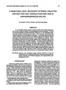
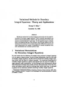
arithmetic operations for the sum and the same number of evaluations of the kernel function KA(s). In our program, `0 = 16; and it can be reset by changing the variable M 0 � 2`0 in the DATA statement of EVALU. If the approximate solution un;m(A) is to be evaluated at a very large number of points A, then this can be an expensive proposition, especially if some of the points A are close to the boundary ?. Again, however, the trapezpoidal rule converges very rapidly if one wishes high accuracy. 5. Numerical examples. For our examples, we use three boundary curves: an ellipse, the ovals of Cassini, and an \amoeba". For the ellipse, the boundary parameterization is simply (55) r(s) = (a cos s; b sin s) ; 0 � s � 2� with a; b > 0. For the ovals of Cassini, the boundary parameterization is r(s) = Rq(s) (cos s; b sin s) (56) p R(s) = cos (2s) + a ? sin2 (2s); 0 � s � 2� with a > 1, b > 0. The ovals of Cassini with (a; b) = (1:1; 1) is shown in Figure 1. The \amoeba" boundary is de ned by r(s) = R(s) (cos s; sin s) (57) R(s) = ecos s cos2 (2s) + esin s sin2 (2s) ; 0 � s � 2� and its graph is shown in Figure 2. Its interior is a decidedly nonconvex and complicated region, and we use it to illustrate that our programs can handle solutions on such unusual boundaries. In evaluating the function u(x; y); we choose a radial grid of test points. It is de ned for the interior Dirichlet problem as follows. �j = 2nj� ; j = 0; :::; n� ? 1 �� � �� k k (58) �k = n + 1 2 ? n + 1 ; k = 1; :::; nr r r Pj;k = �k r(�j ) along with the origin P = (0; 0). The number �k is a measure of how close Pj;k is to the boundary point r(�j ); and �k is an increasing function of k. Also, note that �nr = 1 ? 1 2 (nr + 1) If nr is even moderately large, some of the points Pj;k will be quite close to the boundary. With the Neumann method we use the slight modi cation �j = 2nj� ; j = 0; :::; n� ? 1 � � � �� k k (59) �k = n 2 ? n ; k = 1; :::; nr r r Pj;k = �k r(�j ) 14
1 y 0.5
x
0
−0.5
−1 −1
−0.5
0
0.5
1
. Ovals of Cassini with (a; b) = (1:1; 1)
Fig. 1
which includes points on the boundary ?. For exterior problems, we de ne �k and �j as above, and then we de ne Pj;k = �1 r(�j ) k We also include a very distant point, to approximate a point at 1. The test program is designed to work with any region which is starlike with respect to the origin, and we have used it with regions other than those discussed here. As test problems, we have used the following. � Dirichlet problem: Interior Problem: u(1) = ex cos y �
Exterior Problem:
� Neumann problem:
u(2)
�
�
= exp 2 x 2 cos 2 y 2 x +y x +y
Interior Problem: u(3) = ex cos y ? 1 Exterior Problem: u(4) = x2 +x y2 15
�
2
y
1.5 1 0.5 x
0 −0.5 −1 −1
0
1
2
. The \amoeba" boundary
Fig. 2
These are well-behaved functions, but they will still adequately test the procedures when combined with boundaries ? that are more ill-behaved. We have, of course, used other test functions in addition to the ones given above. The function u(2) is the result of applying the Kelvin transformation (35) to u(1). 5.1. The Dirichlet problem. There is a great deal of data to be presented, and a combination of graphical and tabular forms seems best. We give detailed results for solving the interior Dirichlet problem for u(1) at the points P0;k , k = 0; 1; :::; nr [with P0;0 = (0; 0)]. The parameter " refers to the desired error tolerance, and n is the nal order of the linear system used in INTEQN to calculate the density function �. The number of quadrature points used in obtaining the solution is m, and it varies with the point P1;k . Table 1 contains results for the ellipse with (a; b) = (1; 5), with error tolerances of " = 10?3 and 10?7. The columns labeled Error and PredErr give the actual error and the predicted error bound. PredErr is obtained by combining the error estimates from INTEQN and EVALU, using EST from (41) and the numerical integration error estimate from (49). Figure 3 gives the plots the predicted and actual errors as a function of �k ; or more precisely, we plot
f�k g vs. flog10 jEk jg ; k = 0; 1; :::; nr 16
Table 1
Interior Dirichlet problem on an ellipse - Selected errors " = 10?3 n = 64 " = 10?7
�k m u .000 128 1.0000 .210 128 1.2335 .395 128 1.4845 .556 256 1.7429 .691 256 1.9964 .802 256 2.2310 .889 512 2.4324 .951 1024 2.5873 .988 2048 2.6849
Error ?4:85E ? 11 ?2:51E ? 9 ?1:78E ? 7 ?7:21E ? 11 ?3:46E ? 8 ?4:36E ? 6 ?3:92E ? 7 ?2:77E ? 7 ?2:76E ? 6
PredErr 6:99E ? 5 8:29E ? 5 1:80E ? 4 6:85E ? 5 8:31E ? 5 3:14E ? 4 1:02E ? 4 8:33E ? 5 9:23E ? 5
m 256 256 256 512 512 1024 1024 2048 8192
n = 128
Error 1:44E ? 15 ?4:22E ? 15 ?2:84E ? 14 2:89E ? 15 ?5:33E ? 15 2:22E ? 15 ?4:38E ? 12 ?1:11E ? 11 ?7:10E ? 13
PredErr 1:62E ? 10 4:36E ? 10 1:99E ? 8 1:64E ? 10 4:00E ? 9 1:76E ? 10 4:37E ? 8 3:10E ? 8 2:09E ? 9
with Ek both the predicted error and the actual error. Figure 4 gives graphs of
f�k g vs. flog10 ju(Pj;k) ? un;m(Pj;k)jg ; k = 0; 1; :::; nr for selected j , with " = 10?3. The program DRCHLT used the normal error estimates based on (43) and (50), and the grid parameters inside were n� = 7; nr = 8. All computations were carried out on an HP 720 workstation. Timings are omitted, in part because they were never more than a few seconds, and in part because timings on a workstation network with many users are unreliable. We solved the same interior Dirichlet problem, but on the \amoeba" boundary of Figure 2. When requesting an error tolerance of " = 10?4 and when solving at the points of (58) for (n� ; nr ) = (7; 8), we obtained very regular behaviour in the error in the approximate values of u(1) . The nal number of nodes used in INTEQN was n = 256. At all points P 2 , the predicted error bound for u(Pj;k ) ? un;m(Pj;k) was less than the requested error bound; and the actual errors were always smaller than the predicted error bound, usually much smaller. We also solve an exterior Dirichlet problem on the elliptical region used above. In this case, the boundary ?e obtained by inverting ? thru the unit circle is somewhat ill-behaved, as can be seen in Figure 5. The test function is u(2) , and the other problem parameters are as before. The density function is shown in Figure 6 (with periodic extension to a larger interval), and it is clearly fairly ill-behaved around s = 0. The analogue of Figure 3 is given in Figure 7; and again the predicted error bound satis es the given error tolerance. For the desired error tolerances of " = 10?3; 10?7, the nal values of n used in INTEQN were 256 and 512, respectively. The \normal" error test was used. 5.2. The Neuman problem. The principal di�erences in NEUMAN as compared to DRCHLT are as follows: (i) the error bound (27) has been changed; (ii) the Kelvin transform is now used to convert the interior Neumann problem to an exterior Neumann problem; and (iii) the potential u(P ) can now be evaluated at points P on the boundary 17
−2
10
−4
10
−6
10
−8
10
−10
10
−12
10
Prederr: Eps=1.0E−3 Error: Eps=1.0E−3 Prederr: Eps=1.0E−7 Error: Eps=1.0E−7
−14
10
−16
10
0
0.2
0.4
0.6
0.8
1
. Predicted and actual errors along the radial line � = 0 for a Dirichlet problem on an ellipse
Fig. 3
?. We illustrate NEUMAN by solving the exterior Neumann problem on the ovals of Cassini shown in Figure 1, with boundary data generated from the test case u(4) and with error tolerances of " = 10?3 and 10?7. The points P at which the problem is solved are given in (59), which includes boundary points on ?; and for the parameters de ning P , we used (n� ; nr ) = (7; 8). The analogue of Figure 7, for errors along the line � = 0, is given in Figure 8; and again the predicted error bound satis es the given error tolerance. For the desired error tolerances of " = 10?3; 10?7, the nal values of n used in INTEQN were 128 and 256, respectively. 5.3. Details on computers used in testing. The programs DRCHLT and NEUMAN were tested on several workstations and on a PC using MS Fortran 77. The workstations used were a Hewlett-Packard 720, a Hewlett-Packard C200, an SGI O2, and an IBM RS/6000. The rst three used the Fortran 90 compiler delivered by the manufacturers of the machines, and the last used a Fortran 77 compiler, again supplied by the manufacturer. The examples of this paper are from the HP 720 using Fortran 90 and the default options.
18
σ
−3
10
−4
10
j=0 j=1 j=2
−5
10
−6
10
−7
10
−8
10
−9
10
−10
10
−11
10
−12
10
0
0.2
0.4
0.6
0.8
1
σ
. Errors along selected radial lines � = �j for a Dirichlet problem on an ellipse
Fig. 4
REFERENCES [1] E. Anderson, Z. Bai, C. Bischof, J. Demmel, J. Dongarra, J. DuCroz, A. Greenbaum, S. Hammarling, A. Mckenney, S. Ostrouchov, and D. Sorenson (1992), LAPACK Users' Guide, SIAM Publications, Philadelphia. [2] K. Atkinson (1976) A Survey of Numerical Methods for the Solution of Fredholm Integral Equations of the Second Kind, SIAM Pub. [3] K. Atkinson (1989) An Introduction to Numerical Analysis, 2nd ed., John Wiley and Sons, New York. [4] K. Atkinson (1997) The Numerical Solution of Integral Equations of the Second Kind, Cambridge University Press, Cambridge, UK. [5] R. Kress (1989) Linear Integral Equations, Berlin, Springer. [6] W. Mclean (1985)Boundary Integral Equation Methods for the Laplace Equation Ph.D thesis, Australian National University, Canberra. [7] C. Miller (1979) Numerical Solution of Two-Dimensional Potential Theory Problems Using Integral Equation Techniques, Ph.D thesis, University of Iowa, Iowa City. [8] NAG Library (1993) D03EAF, a program description. [9] I. Petrovskii (1967) Partial Di�erential Equations, W. B. Saunders, Co. [10] P. Swarztrauber (1982), Vectorizing the FFT's, in Parallel Computations, G. Rodrigue (editor), Academic Press, New York, pp. 51-83. (Available from the NETLIB library.)
19
y 0.5
x
0
−0.5
−1
−0.5
0
0.5
1
. Boundary ?e for ellipse with (a; b) = (1; 5) inverted thru unit circle
Fig. 5
20
0.1 0 −0.1 −0.2 −0.3 −0.4 −0.5 −0.6 −0.7 −2
s 0
2
4
6
8
. The density �(s) on ?e for exterior Dirichlet problem de ned originally outside an ellipse
Fig. 6
21
−2
10
−4
10
−6
10
−8
10
−10
10
−12
10
Prederr: Eps=1.0E−3 Error: Eps=1.0E−3 Prederr: Eps=1.0E−7 Error: Eps=1.0E−7
−14
10
−16
10
0
0.2
0.4
0.6
0.8
Fig. 7. Predicted and actual errors along the radial line � = 0 for an exterior Dirichlet problem on an ellipse
22
1
1/ σ
−2
10
−4
10
−6
10
−8
10
−10
10
Prederr: Eps=1.0E−3 Error: Eps=1.0E−3 Prederr: Eps=1.0E−7 Error: Eps=1.0E−7
−12
10
−14
10
−16
10
0
0.2
0.4
0.6
0.8
1
1/ σ
Fig. 8. Predicted and actual errors along the radial line � = 0 for an exterior Neumann problem on an \ovals of Cassini"
23