Solving the hypersingular boundary integral equation in three

Solving the hypersingular boundary integral equation in three-dimensional acoustics using a regularization relationship Zai You Yan, Kin Chew Hung,a) and Hui Zheng Institute of High Performance Computing, 1 Science Park Road #01-01 The Capricorn, Singapore Science Park II, Singapore 117528

共Received 2 August 2002; revised 2 January 2003; accepted 24 January 2003兲 Regularization of the hypersingular integral in the normal derivative of the conventional Helmholtz integral equation through a double surface integral method or regularization relationship has been studied. By introducing the new concept of discretized operator matrix, evaluation of the double surface integrals is reduced to calculate the product of two discretized operator matrices. Such a treatment greatly improves the computational efficiency. As the number of frequencies to be computed increases, the computational cost of solving the composite Helmholtz integral equation is comparable to that of solving the conventional Helmholtz integral equation. In this paper, the detailed formulation of the proposed regularization method is presented. The computational efficiency and accuracy of the regularization method are demonstrated for a general class of acoustic radiation and scattering problems. The radiation of a pulsating sphere, an oscillating sphere, and a rigid sphere insonified by a plane acoustic wave are solved using the new method with curvilinear quadrilateral isoparametric elements. It is found that the numerical results rapidly converge to the corresponding analytical solutions as finer meshes are applied. © 2003 Acoustical Society of America. 关DOI: 10.1121/1.1560164兴 PACS numbers: 43.40.Rj, 43.20.Rz, 43.20.Fn 关EGW兴

I. INTRODUCTION

Boundary element method based on the Helmholtz integral equation has long been applied for the analysis of acoustic radiation and scattering problems. Its significant advantages over other popular numerical techniques such as the finite difference and finite element method include a reduction of dimensionality of the problem by one, and an automatic satisfaction of the radiation boundary condition. However, the classical boundary element method for exterior acoustic problems fails to provide a unique solution at certain frequencies, which are the characteristics of the associated interior problem. The nonuniqueness is a purely mathematical problem arising from the boundary integral formulation rather than from the nature of the physical problem. A detailed description about the nonuniquness problem is presented in Ref. 1. Several modified integral formulations have been developed to overcome the nonuniqueness problem. By far, the combined Helmholtz integral equation formulation 共CHIEF兲 proposed by Schenck2 in 1968 and the composite Helmholtz integral equation 共CHIE兲 presented by Burton and Miller3 in 1971 are the two most popular approaches. In the CHIEF method, Schenck2 combined the surface Helmholtz integral equation with the interior Helmholtz integral equation to form an overdetermined system of equations, which was then solved using the least-squares procedure. Seybert et al.4 provided a computational method based on the CHIEF method using isoparametric element formulation. Recently, Chen et al.5 extended the CHIEF method to the combined Helma兲

Electronic mail: [email protected]

2674

J. Acoust. Soc. Am. 113 (5), May 2003

holtz exterior integral equation formulation to solve the interior problems. Although the CHIEF method is very simple to implement, it fails when the interior points are located on a nodal surface of the corresponding interior problem. To date, the selection of some suitable interior points still remains as a difficult problem. On the other hand, the CHIE method uses a linear combination of the Helmholtz integral equation and its normal derivative equation. It was proved that the linear combination of these two integral equations would yield a unique solution for all frequencies with a suitable complex combination coefficient, even if both the Helmholtz integral equation and its normal derivative equation suffer from the nonuniqueness problem. This method appears to be robust for numerical implementation. However, it suffers from a major drawback that hypersingular integral is involved in the normal derivative of the Helmholtz integral equation. Numerical techniques for computing nonsingular, nearly singular, and nearly hypersingular integrals can be found in the review paper by Tanaka et al.6 Burton and Miller3 used a double surface integral method throughout the integral equation to reduce the order of the hypersingularity. Although such a technique results in numerically tractable kernels, it is computationally expensive to evaluate a double surface integral. The regularization techniques developed by Meyer et al.7 and Terai8 are valid for planar element only. Mathews9 compared the double surface integral method3 and the regularization technique7 using quadratic quadrilateral isoparametric elements. It was noted that the regularization technique resulted in 1/r type singular integrals over the element near the point of singularity, even if a polar coordinate transformation was employed. Chien et al.10 developed an approach to regularize such hypersin-

0001-4966/2003/113(5)/2674/10/$19.00

© 2003 Acoustical Society of America

gular integrals by employing certain known identities from the associated interior Laplace problems. Adaptive subdivision around singular points was needed in the numerical computation. Yang11 successfully implemented this method in the study of acoustic scattering across a wide frequency range. Liu and Rizzo12 developed a general form of the hypersingular boundary integral equation, which contained at most weakly singular integrals. This weakly singular form was derived by employing certain integral identities involving the static Green’s function. Recently, Liu and Chen13 made an improvement on this method with a new formulation that involves only tangential derivatives of the density function. Especially, C 0 continuous boundary elements were employed in the discretization. Wu et al.14 implemented a regularized normal derivative equation, which converges in the Cauchy principal value sense rather than in the finite-part sense. This equation required the evaluation of tangential derivatives everywhere on the boundary. By taking the advantage of the properties of axisymmetric geometry, Wang et al.15 successfully computed the hypersingular integrals using tangential operators. But this approach can only be applied to the problems with axisymmetric geometry. Hwang16 regularized the hypersingular Helmholtz integral equation by some identities from the associated Laplace equations. The collocation points were chosen to be the Gauss–Legendre nodes and no interpolation function was assumed for acoustic variables. In that study, an important assumption was that the normal derivative of the dimensionless solid angle was identical to zero as point was on the surface. On the other hand, source distribution for the equipotential surface from the potential theory was employed to regularize the weak singularities. Therefore, the value of equipotential inside the domain must be calculated. A mathematical investigation about the existence of uniqueness theorems of the boundary element methods based on the Helmholtz integral equation was performed by Luke and Martin.17 They also discussed the treatment of the hypersingular integral by the double surface integral method. In this paper, the regularization of the hypersingular integral in the CHIE method is investigated through the double surface integral method. As stated earlier, it is computationally expensive to evaluate a double surface integral. Now by introducing the new concept of discretized operator matrix, evaluation of the double surface integral is reduced to the evaluation of the two discretized operator matrices. As a result, the computational cost for calculating CHIE is comparable to that of solving the conventional Helmholtz integral equation as the number of frequencies to be computed increases. This paper is organized into five sections. Following the Introduction, a detailed theoretical formulation of the governing equation for acoustic propagation in unbounded exterior domain is presented. Next, a discretization scheme for the surface boundary integral equations using a set of curvilinear quadrilateral isoparametric elements is discussed. A new concept of discretized operator matrix is introduced here. The double surface integral is discretized according to this new concept and the discretized operator matrix of the hypersingular integral operator N 0 is found. The hypersingularity in the integral operator N k is eliminated using the opJ. Acoust. Soc. Am., Vol. 113, No. 5, May 2003

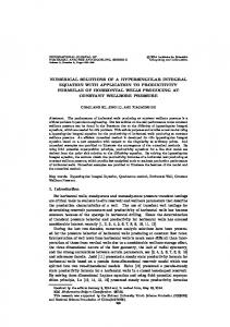
FIG. 1. Notation for a structure with smooth surface.

eration N k ⫺N 0 . Then, numerical calculations are performed for pulsating and oscillating sphere radiation and plane acoustic wave scattering from a rigid sphere. Three kinds of surface Helmholtz integral equations have been solved. They are the conventional Helmholtz integral equation 共HIE兲, the normal derivative of the conventional Helmholtz integral equation 共NDHIE兲, and the composite Helmholtz integral equation 共CHIE兲. Finally a conclusion is drawn.

II. THEORETICAL DEVELOPMENT

Consider the acoustic pressure field in the exterior unbounded domain E. The acoustic field is either radiated by a finite body with smooth surface S vibrating with prescribed velocity distribution or scattered of acoustic waves from rigid surface S. The exterior infinite fluid medium is assumed to be homogeneous. Sound travels in the fluid medium with speed c and the fluid density is ␳. The normal vector at any point on the surface is taken to be the inward normal as shown in Fig. 1. The governing differential equation1 of the exterior acoustic domain in steady-state linear acoustics is the wellknown Helmholtz equation, 共 ⵜ 2 ⫹k 2 兲 ␸ ⫽0.

共1兲

The Neumann boundary condition on the boundary surface S can be expressed as

⳵␸ ⫽i ␻␳ v n . ⳵n

共2兲

In case of acoutic radiation, the acoustic pressure ␸ must satisfy the Sommerfeld radiation condition at infinity, lim r→⬁

冕冕冉 ⳵␸⳵ r

⫹ikr

冊

2

dS⫽0,

共3兲

where ␸ represents the acoustic pressure, ␻ represents the circular frequency, k is the wave number, and v n denotes the normal surface velocity. By using the Green’s second identity, the surface Helmholtz integral equation that satisfies the Sommerfeld radiation condition is Yan et al.: Evaluation of hypersingular integral equation

2675

冕冕冉␸

共q兲

冊

⳵ G k 共 p,q 兲 ⳵␸ 共 p 兲 1 ⫺G k 共 p,q 兲 dS q ⫽ ␸ 共 p 兲 . ⳵nq ⳵nq 2

Therefore, the composite integral operators L 0 N 0 and M 20 are defined as 共4兲

The free-space Green’s function G k for the threedimensional wave equation is G k 共 p,q 兲 ⫽e ⫺ikr /4␲ r,

共5兲

r⫽ 兩 p⫺q 兩 ,

where p is the source point anywhere on the surface, and q is the field point on the surface, see Fig. 1. r represents the Euclidean distance between points p and q. In operator notation,8 Eq. 共5兲 can be written as

冋

册

⳵␸ 1 ⫺ I⫹M k ␸ ⫽L k , 2 ⳵n

共6兲

where L k␮ ⫽

冕冕␮ 冕冕␮

共7兲

冎再冋

1 1 ⫺ I⫹M k ⫹ ␣ N k ␸ ⫽ L k ⫹ ␣ I⫹M Tk 2 2

共8兲

册冎

⳵␸ , ⳵n

共9兲

where ␣, the coupling constant, is chosen to be strictly complex when wave number k is a real number. Here ␣ takes the value ⫺i/k. The integral operators N k and M Tk can be expressed as N k␮ ⫽

冕冕␮ 冕冕␮

M Tk ␮ ⫽

共q兲

⳵ 2 G k 共 p,q 兲 dS q , ⳵ n p⳵ n q

共q兲

⳵ G k 共 p,q 兲 dS q . ⳵np

共10兲

The main drawback of the CHIE method is the numerical treatment of the hypersingular integral kernel N k that appears in the normal derivative equation. Burton and Miller3 used a regularization relationship, which replaces a hypersingular integral operator with two weakly singular integral operators, to deal with the hypersingularity in operator N k . The regularization relationship used is L 0 N 0 ⫽ 关 M 0 ⫹ 21 I 兴关 M 0 ⫺ 12 I 兴 ⫽M 20 ⫺ 14 I,

共11兲

where L 0 , N 0 , and M 0 are integral operators identical to L k , N k , and M k except that the kernels of L 0 , N 0 , and M 0 contain G 0 (p,q)⫽1/4␲ r not G k . 2676

再冕冕 ⳵⳵ 2

G 0 共 p,q 兲

冕冕⳵ ⳵

G 0 共 p,q 兲 nq

再冕冕

冎冎

G 0 共 q,t 兲 ␮ 共 t 兲 dS t dS q , n q⳵ n t 共12兲

⳵ G 0 共 q,t 兲 ␮ 共 t 兲 dS t dS q . ⳵nt 共13兲

According to the regularization relationship, Eq. 共11兲, Burton and Miller3 developed the following transformation to remove the hypersingularity in the operator N k : L 0 N k ⫽L 0 关 N k ⫺N 0 兴 ⫹L 0 N 0 ⫽L 0 关 N k ⫺N 0 兴 ⫹M 20 ⫺ 41 I, 共14兲 L 0 关 N k ⫺N 0 兴 ␮ 共 p 兲 ⫽

⳵ G k 共 p,q 兲 dS q . 共q兲 ⳵nq

It is well known that the above surface Helmholtz integral equation, Eq. 共4兲, leads to nonuniqueness solutions at certain frequencies that are the characteristics of the associated interior problem. As discussed in Sec. I, remedies to resolve the problem of nonuniqueness have been investigated by many researchers. Here, the CHIE method is studied. The CHIE method is based on a linear combination of the surface Helmholtz integral equation, Eq. 共4兲, and its normal derivative with respect to the source point. The resulting equation was proven to have unique solutions at all wave numbers, which can be expressed in operator notation as

再

M 20 ␮ 共 p 兲 ⫽

冕冕

where

共 q 兲 G k 共 p,q 兲 dS q ,

M k␮ ⫽

L 0N 0␮共 p 兲⫽

J. Acoust. Soc. Am., Vol. 113, No. 5, May 2003

冕冕冋冕冕 ⳵

G 0 共 p,q 兲 2

⫻

册

关 G 共 q,t 兲 ⫺G 0 共 q,t 兲兴 ␮ 共 t 兲 dS t dS q . ⳵ n t⳵ n q

共15兲

Then the CHIE in Eq. 共9兲 was rewritten as L 0 兵 ⫺ 21 I⫺M k ⫹ ␣ 共 N k ⫺N 0 兲其 ␸ ⫹ ␣ 关 M 20 ⫺ 41 I 兴 ␸

再冋

⫽L 0 L k ⫹ ␣

1 I⫹M Tk 2

册冎

⳵␸ . ⳵n

共16兲

In Eq. 共16兲, the hypersingular integral operator N k has been transformed into several weakly singular integral operators. However, the composite integral operators, such as L 0 关 N k ⫺N 0 兴 and M 20 , are double surface integrals and these integrals must be computed for each frequency step. It is very inefficient to numerically implement such an approach. Therefore, even though it gives rise to tractable kernels, it is abandoned by most of the researchers. In this paper, the regularization relationship, Eq. 共11兲, will be applied. A new method is proposed to discretize it. Finally a highly efficient approach is developed to solve the hypersingular integral.

III. DISCRETIZATION OF THE INTEGRAL OPERATORS

The integral operators are discretized using eight-noded, quadratic quadrilateral isoparametric surface elements which allows the integration of the interpolated variables over a three-dimensional surface to be carried out within a standard basis square in the 共␰,␩兲 local coordinate space. The global Cartesian coordinates x are related to the nodal global coordinates x i by 8

x共 ␰,␩ 兲⫽

兺 N i共 ␰ , ␩ 兲 x i .

i⫽1

共17兲

N i ( ␰ , ␩ ) is the shape function8 for the quadratic quadilateral elements with nodes numbered in counterclockwise fashion. The acoustic variables ␸ and ⳵␸ / ⳵ n are approximated over each element by the shape functions, that is, Yan et al.: Evaluation of hypersingular integral equation

TABLE I. Comparison of computational time for different methods. Model

Method

Per frequency step 共s兲

For N 0 operator 共s兲

24-element

Double surface integral 关Eq. 共16兲兴 Proposed method 关Eq. 共35兲兴 HIE 关Eq. 共6兲兴 Double surface integral 关Eq. 共16兲兴 Proposed method 关Eq. 共35兲兴 HIE 关Eq. 共6兲兴

148.751 67 1.081 555 2 1.041 497 7 8290.458 12.998 693 12.818 431

x 0.751 080 0 x x 8.752 585 x

96-element

8

8

␸⫽

兺

i⫽1

N i␸ i ,

⳵␸ ⳵␸ i ⫽ , Ni ⳵ n i⫽1 ⳵n

兺

共18兲

where ␸ i represents the nodal quantity of the variable ␸. With these relationships, integration of the integral operator L k expressed in Eq. 共7兲 can be discretized using n elements as follows: L k␸ ⫽

冕冕

Similarly, the discretized operator matrix A k for the integral operator M k is expressed as A ki,m ⫽

m⫽ f 共 j,l 兲

冕冕

⫽

兺兺冕冕G k共 p,q 兲 N i共 ␰ , ␩ 兲 J 共 ␰ , ␩ 兲 d ␰ d ␩ ␸ i j⫽1 i⫽1

兺

冕冕

D 0i,m ⫽

8

⌬S j

⫽B k 兵 ␸ 其 ,

共19兲

兺

m⫽ f 共 j,l 兲

B ki,m ⫽

兺冕冕N l G ki j dS q , m⫽ f 共 j,l 兲

N l G 0i j 共 p,q 兲 dS q ,

⌬S j

共22兲

⳵ 2 G 0i j 共 p,q 兲 N l dS q . ⳵ n p⳵ n q

⌬S j

In the past, the composite integral operator L 0 N 0 in Eq. 共12兲 was directly approximated as n

where 兵 ␸ 其 ⫽ 关 ␸ 1 , ␸ 2 , . . . K, ␸ t 兴 T , t is the total global node number. The square matrix B k is defined as the discretized operator matrix of the integral operator L k ,

共21兲

and that for the discretized operator matrices B 0 and D 0 of the integral operators L 0 and N 0 are

S n

⳵ G ki j dS q , ⳵n

⌬S j

B 0i,m ⫽

Gk共 p,q兲␸共q兲dSq

兺冕冕N l m⫽ f 共 j,l 兲

L 0N 0␮ i共 p 兲 ⫽

兺

j⫽1

⫻ 共20兲

⌬S j

再

冕冕 ⌬S j n

兺

l⫽1

where the function f ( j,l) is the mapping function for the relation between element nodes and global nodes. Comparing Eq. 共20兲 and Eq. 共7兲, it is evident that the element of the discretized operator matrix takes the same integral form as the integral operator.

冕冕

n

8

兺兺兺

j⫽1 l⫽1 k⫽1

⫻

再

8

兺

冕冕

G 0i j 共 p,q 兲

⌬S j

冕冕 ⳵ ⳵ 2

冎

⳵ 2 G 0 jl 共 q,t 兲 N ␮ dS dS q ⳵ n q ⳵ n t k⫽1 k k t

⌬Sl

n

⫽

G 0i j 共 p,q 兲

冎

G 0 jl 共 q,t 兲 N k dS t dS q ␮ k , n q⳵ n t

⌬Sl

共23兲

which is obviously too computationally expensive to evaluate, and has deterred from implementing the regularization relationship, Eq. 共11兲. In this study, a new idea is proposed to discretized the composite integral operator L 0 N 0 . Assuming that

␺共 q 兲⫽

冕冕

⳵2G0共q,t兲 ␮共t兲dSt , ⳵nq⳵nt

共24兲

S

over each element, using the shape functions N l , we have 8

␺ ⫽ 兺 N l␺ l , l⫽1

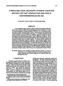
FIG. 2. Surface discretization of one octant of a sphere using 3 curvilinear quadrilateral elements. J. Acoust. Soc. Am., Vol. 113, No. 5, May 2003

共25兲

where ␺ l is nodal value of function ␺. Based on the definition of discretized operator matrix, Eq. 共24兲 can be disYan et al.: Evaluation of hypersingular integral equation

2677

FIG. 3. Surface discretization of one octant of a sphere using 12 curvilinear quadrilateral elements.

cretized and expressed in the form of discretized operator matrix,

兵 ␺ 其 ⫽D 0 兵 ␮ 其 ,

共26兲

where 兵␺其 and 兵␮其 are values at global nodes, and are constants in the integration. D 0 is the discretized operator matrix of integral operator N 0 . Because N 0 is a hypersingular integral operator and the integral does not exist in either conventional or Cauchy-principal value sense. The operator matrix D 0 should be obtained in the Hadamard finite part sense.16 Substituting Eq. 共24兲 into Eq. 共12兲, we have L 0N 0␮共 p 兲⫽

冕冕

G0共 p,q兲␺共q兲dSq .

共27兲

S

The discretization of Eq. 共27兲 can be expressed in discretized operator matrix form as E 0 兵 ␮ 其 ⫽B 0 兵 ␺ 其 ,

共28兲

where E 0 is the discretized operator matrix of the composite integral operator L 0 N 0 . Substituting Eq. 共26兲 into Eq. 共28兲, we have

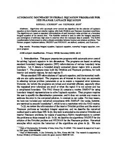
FIG. 5. Dimensionless surface acoustic pressures from a pulsating sphere using CHIE with 24 elements.

cretized operator matrix E 0 is equal to the product of B 0 and D0 , E 0 ⫽B 0 D 0 .

共30兲

The discretized operator matrix A 20 corresponding to the composite integral operator M 20 can be obtained in the same way. A 0 is the discretized operator matrix of integral operator M0 , A 0,im ⫽

兺冕冕N l m⫽ f 共 j,l 兲

⳵ G 0i j dS q . ⳵n

共31兲

⌬S j

Therefore, the regularization relationship, Eq. 共11兲, can be expressed in the form of discretized operator matrices as B 0 D 0 ⫽A 20 ⫺ 41 I.

共32兲

Then, we have 1 2 D 0 ⫽B ⫺1 0 共 A 0⫺ 4I 兲.

共33兲

Because the regularization relationship, Eq. 共11兲, is an identity formulation and ␮ is an arbitrary function, the dis-

Now the double surface integrations in the regularization relationship, Eq. 共11兲, have been reduced to the product of surface integrations. Above all, the discretized operator matrix of the hypersingular integral operator N 0 as higher-order elements are implemented is explicitly found for the first time.

FIG. 4. Dimensionless surface acoustic pressures from a pulsating sphere using HIE and NDHIE with 24 elements.

FIG. 6. Dimensionless surface acoustic pressures from a pulsating sphere using HIE and NDHIE with 96 elements.

E 0 兵 ␮ 其 ⫽B 0 D 0 兵 ␮ 其 .

2678


共29兲

Yan et al.: Evaluation of hypersingular integral equation

D im ⫽

F im ⫽

FIG. 7. Dimensionless surface acoustic pressures from a pulsating sphere using CHIE with 96 elements.

IV. TREATMENT OF THE HYPERSINGULARITY IN OPERATOR N k

Now applying the integral operator N 0 , Eq. 共9兲 can be modified as 关 ⫺ 12 I⫹M k ⫹ ␣ 关共 N k ⫺N 0 兲 ⫹N 0 兴兴 ␸

冋冋

⫽ L k⫹ ␣

1 I⫹M Tk 2

册册

⳵␸ . ⳵n

共34兲

The term (N k ⫺N 0 ) has removed the hypersingularity in operator N k . Only the term N 0 still contains hypersingularity. Using the discretized operator matrices, Eq. 共34兲 can be discretized and expressed as

冋

册冋冋

1 1 ⫺ I⫹A k ⫹ ␣ 关 D⫹D 0 兴兵 ␸ 其 ⫽ B k ⫹ ␣ I⫹F 2 2

册册再冎

⳵␸ , ⳵n 共35兲

where D is the discretized operator matrix for integral operator (N k ⫺N 0 ) and F is the discretized operator matrix of integral operator M Tk ,

兺

m⫽ f 共 j,l 兲

兺

m⫽ f 共 j,l 兲

冕冕

Nl

⳵ 2 共 G ki j ⫺G 0i j 兲 dS q , ⳵ n t⳵ n q

⌬S j

冕冕

Nl

⳵ G 0i j 共 p,q 兲 dS q . ⳵np

共36兲

⌬S j

Since the discretized operator matrix D 0 of the hypersingular integral operator N 0 has already been obtained by Eq. 共33兲, the linear equation system in Eq. 共35兲 can be numerically solved using a weakly singular integration scheme, such as that proposed by Lachat and Watson.18 As the discretized operator matrix D 0 is independent of frequency, the computational cost of solving Eq. 共35兲 is comparable to that of solving the conventional Helmholtz integral equation, Eq. 共6兲, as the number of frequencies to be computed increases. Table I presents the computational time for solving the problem of pulsating sphere radiation, which will be described in detail in Sec. V, using different methods. Here the computer is a Dell Latitude C610 notebook. Clearly, the new approach greatly improves the computational efficiency as compared to the technique applied in Eq. 共16兲. For each frequency step, the computational time for the new method is very close to that for the HIE Eq. 共6兲. V. NUMERICAL EXAMPLES

In order to test the accuracy and efficiency of the new method, two cases of acoustic radiation and a case of plane acoustic wave scattering from rigid sphere have been computed. The two acoustic radiation problems are pulsating sphere radiation and oscillating sphere radiation. In all three examples, the surface of a sphere is, respectively, modeled using 24 and 96 curvilinear quadrilateral isoparametric elements to observe the convergence of the new method. Each octant of a sphere is discretized using 3 and 12 surface elements as shown in Figs. 2 and 3. Due to symmetry, the problems are computed in half space. For radiation problems, three linear equation systems are computed. They are the conventional Helmholtz integral equation 共HIE兲, normal derivative equation of the conventional Helmholtz integral equation 共NDHIE兲, and the composite Helmholtz integral equation 共CHIE兲. Comparisons between the numerical results of these three linear equation systems clearly show the nonuniqueness problem and the effectiveness of the new method. For plane acoustic wave scattering from a rigid sphere, only the conventional Helmholtz integral equation and the composite Helmholtz integral equation are computed. These examples are computed using the in-house developed code, SSFI. This software is suitable to solve multidomain acoustic problems, especially the problems of structural–acoustic interaction. A. Pulsating sphere radiation

The analytical solution10 of the acoustic pressure ␸ (r) for a sphere of radius a, pulsating with an uniform radial velocity v 0 , is given by FIG. 8. Dimensionless surface acoustic pressures for an oscillating sphere using HIE and NDHIE with 24 elements as ␪ ⫽0°.

␸ 共 r 兲 a ika ⫽ e ⫺ik 共 r⫺a 兲 . ␳ c v 0 r 1⫹ika

共37兲



2679

FIG. 9. Dimensionless surface acoustic pressures for an oscillating sphere using CHIE with 24 elements as ␪ ⫽0°.

Dimensionless surface acoustic pressures as a function of the reduced frequency ka are plotted in Figs. 4 –7. Figures 4 and 5 present the results obtained using 24 elements. While the numerical results obtained using 96 elements are presented in Figs. 6 and 7. The comparison between the numerical results obtained using the HIE and NDHIE with the corresponding analytical solutions is shown in Figs. 4 and 6. It is evident that the HIE equation fails to provide unique solutions near ka⫽ ␲ , 2␲, 8.13, and 3␲ and the NDHIE equation fails to provide unique solutions near ka⫽0, 4.493, 5.616, 7.725, and 9.784. On the other hand, the numerical results calculated using the CHIE, which are plotted in Figs. 5 and 7, are unique for all the frequencies. Figure 7 shows that with a finer mesh, the numerical results obtained using the CHIE agree very well with the analytical solutions for ka up to 10.5.

B. Oscillating sphere radiation

The analytical solution10 of the acoustic pressure for an oscillating sphere of radius a with a radial velocity v 0 cos(␪) is given by

冉冊

FIG. 11. Dimensionless surface acoustic pressures for an oscillating sphere using CHIE with 96 elements as ␪ ⫽0°.

where ␪ is the angle made by the radial direction and the direction of the velocity. In the following example, ␪ ⫽0 is along the direction of z axis. The dimensionless surface acoustic pressures at ␪ ⫽0 are displayed as function of the reduced frequency in Figs. 8 –11. Figures 8 and 9 show the results obtained using the model with 24 elements. The results for 96 elements model are shown in Figs. 10 and 11. The comparison between the numerical results obtained using the HIE and NDHIE with the corresponding analytical solutions is shown in Figs. 8 and 10. As can be seen, the HIE equation fails to provide unique solutions near ka⫽4.493, 7.725, and 9.349. Similarly, the NDHIE equation also suffers from the nonuniquness near ka⫽2.062, 5.911, 5.616, 6.787, 8.521, and 9.150, whereas the numerical results calculated using the CHIE displayed in Figs. 9 and 11 are unique for all the wave numbers. Figure 11 shows that with a finer mesh discretization the surface acoustic pressures for an oscillating sphere obtained using the CHIE agree quite well with the corresponding analytical solutions for ka up to 10.5. C. Plane acoustic wave scattering from a rigid sphere

共38兲

To provide a further test of the new technique, the scattering of a plane acoustic wave ␸ I ⫽ ␸ 0 e ⫺ikz from a rigid sphere of radius a is computed. The analytical solution19 of

FIG. 10. Dimensionless surface acoustic pressures for an oscillating sphere using HIE and NDHIE with 96 elements as ␪ ⫽0°.

FIG. 12. The angular dependence of ␸ s / ␸ 0 as ka⫽1.0 and r⫽5a with 24 elements.

␸共 r 兲 a ⫽ ␳cv0 r

2680

2

cos共 ␪ 兲

ika 共 1⫹ikr 兲 e ⫺ik 共 r⫺a 兲 , 2 共 1⫹ika 兲 ⫺k 2 a 2



FIG. 13. The angular dependence of ␸ s / ␸ 0 as ka⫽ ␲ and r⫽5a with 24 elements.

FIG. 16. The angular dependence of ␸ s / ␸ 0 as ka⫽ ␲ and r⫽5a with 96 elements.

FIG. 14. The angular dependence of ␸ s / ␸ 0 as ka⫽4 and r⫽5a with 24 elements.

FIG. 17. The angular dependence of ␸ s / ␸ 0 as ka⫽4 and r⫽5a with 96 elements.





2681

FIG. 19. The angular dependence of ␸ s / ␸ 0 as ka⫽2 ␲ and r⫽5a with 96 elements.

the scattered acoustic pressure ␸ s (r, ␪ ) at a distance r from the center of the sphere and at an angle ␪ from the direction of the incoming wave is given by ⬁

冋

册

tegral equation proposed by Burton and Miller.3 The discretized operator matrix of a composite integral operator is proved to be just the product of the two discretized operator matrices corresponding to the two integral operators, which construct the composite integral operator. The double surface integrals employed by Burton and Miller3 are discretized according to this new concept. Above all, the discretized operator matrix of the hypersingular integral operator N 0 is explicitly found for the first time as higher-order elements are implemented. Subsequently, an elimination of the hypersingularity in the integral operator N k is implemented using the formulation N k ⫺N 0 . The new method greatly improves the computational efficiency and has tractable integral kernels. Numerical calculations are performed for pulsating and oscillating sphere radiation and plane acoustic wave scattering from a rigid sphere with curvilinear quadrilateral isoparametric elements being employed. As finer meshes are applied, the numerical results agree quite well with the corresponding analytical solutions. Here surface of the object is constrained to be smooth enough. Further investigations will extend the new technique to problems with arbitrary shape structure.

⬘ 共 ka 兲 jm ␸ s 共 r, ␪ 兲 ⫽ ⫺ 共 ⫺i 兲 m 共 2m⫹1 兲 h 共 kr 兲 ␸0 ⬘ 共 ka 兲 m hm m⫽0

兺

⫻ P m 共 cos ␪ 兲 ,

共39兲

where j m is spherical Bessel function of the first kind and h m is spherical Hankel function of the second kind. P m denotes Legendre polynomial of order m. Figures 12–14 present the results obtained using the 24element model. While Figs. 15–19 present the results obtained using the 96-element model. The results at r⫽5a are presented. Figures 12 and 15 show the angular dependency of ␸ s / ␸ 0 as ka⫽1.0. It is observed that the numerical results obtained using both the HIE and CHIE agree well with the analytical solutions. Figures 13 and 16 show the results at the reduced frequency ka⫽ ␲ . As ka⫽ ␲ is one of the characteristic frequencies,11 the scattered acoustic pressures obtained using the HIE do not agree with the corresponding analytical solutions. However, the scattered acoustic pressures obtained using the CHIE again agree very well with the analytical solutions. Figures 14 and 17 demonstrate the angular dependency of ␸ s / ␸ 0 at ka⫽4. Comparisons between these two figures indicate that the numerical results converge rapidly as finer meshes are applied. Angular dependencies of ␸ s / ␸ 0 at ka⫽4.493 and 2␲ are presented in Figs. 18 and 19, respectively. These frequencies correspond to the characteristic frequencies of either the conventional Helmholtz integral equation or its normal derivative equation. All these figures demonstrate that the new technique can overcome the nonuniqueness problem encountered in acoustic scattering analysis using the conventional Helmholtz integral equation.

VI. CONCLUSIONS

By introducing the concept of discretized operator matrix, a new method has been generated to overcome the hypersingular integral involved in the composite Helmholtz in2682


1

R. D. Ciskowski and C. A. Brebbia, Boundary Element Methods in Acoustics 共Computational Mechanics, Souththampton, Boston, 1991兲. 2 H. A. Schenck, ‘‘Improved integral formulation for acoustic radiation problems,’’ J. Acoust. Soc. Am. 44, 41–58 共1968兲. 3 A. J. Burton and G. F. Miller, ‘‘The application of integral equation methods to the numerical solution of some exterior boundary value problems,’’ Proc. R. Soc. London, Ser. A 323, 201–210 共1971兲. 4 A. F. Seybert, B. Soenarko, F. J. Rizzo, and D. J. Shippy, ‘‘An advanced computational method for radiation and scattering of acoustic waves in three dimensions,’’ J. Acoust. Soc. Am. 77, 362–368 共1985兲. 5 I. L. Chen, J. T. Chen, S. R. Kuo, and M. T. Liang, ‘‘A new method for true and spurious eigensolutions of arbitrary cavities using the combined Helmholtz exterior integral equation formulation method,’’ J. Acoust. Soc. Am. 109, 982–998 共2001兲. 6 M. Tanaka, V. Sladek, and J. Sladek, ‘‘Regularization techniques applied to boundary element methods,’’ Appl. Mech. Rev. 47, 457– 499 共1994兲. 7 W. L. Meyer, W. A. Bell, and B. T. Zinn, ‘‘Boundary integral solutions of three dimensional acoustic radiation problems,’’ J. Sound Vib. 59, 245– 262 共1978兲. 8 T. Terai, ‘‘On calculation of sound fields around three dimensional objects by integral equation methods,’’ J. Sound Vib. 69, 71–100 共1980兲. 9 I. C. Mathews, ‘‘Numerical techniques for three dimensional steady-state fluid-structure interaction,’’ J. Acoust. Soc. Am. 79, 1317–1325 共1986兲. 10 C. C. Chien, H. Rajiyah, and S. N. Atluri, ‘‘An effective method for solving the hyper-singular integral equations in 3-D acoustics,’’ J. Acoust. Soc. Am. 88, 918 –937 共1990兲. 11 S.-A. Yang, ‘‘Acoustic scattering by a hard and soft body across a wide frequency range by the Helmholtz integral equation method,’’ J. Acoust. Soc. Am. 102, 2511–2520 共1997兲. 12 Y. J. Liu and F. J. Rizzo, ‘‘A weakly-singular form of the hypersingular boundary integral equation applied to 3-D acoustic wave problems,’’ Comput. Methods Appl. Mech. Eng. 96, 271–287 共1992兲. 13 Y. J. Liu and S. H. Chen, ‘‘A new form of the hypersingular boundary integral equation for 3-D acoustics and its implementation with C0 boundary elements,’’ Comput. Methods Appl. Mech. Eng. 173, 375–386 共1999兲. 14 T. W. Wu, A. F. Seybert, and G. C. Wan, ‘‘On the numerical implementation of a Cauchy principal value integral to insure a unique solution for acoustic radiation and scattering,’’ J. Acoust. Soc. Am. 90, 554 –560 共1991兲. 15 W. P. Wang, N. Atalla, and J. Nicolas, ‘‘A boundary integral approach for acoustic radiation of axisymmetric bodies with arbitrary boundary conditions valid for all wave numbers,’’ J. Acoust. Soc. Am. 101, 1468 –1478 共1997兲. Yan et al.: Evaluation of hypersingular integral equation

16

W. S. Hwang ‘‘Hyper-singular boundary integral equations for exterior acoustic problems,’’ J. Acoust. Soc. Am. 101, 3336 –3342 共1997兲. 17 C. J. Luke and P. A. Martin, ‘‘Fluid-solid interaction: Acoustic scattering by a smooth elastic obstacle,’’ SIAM 共Soc. Ind. Appl. Math.兲 J. Appl. Math. 55, 904 –922 共1995兲.


18

J. C. Lachat and J. O. Watson, ‘‘Effective numerical treatment of boundary integral equations,’’ Int. J. Numer. Methods Eng. 10, 991–1005 共1976兲. 19 M. C. Junger, ‘‘Sound scattering by thin elastic shells,’’ J. Acoust. Soc. Am. 24, 366 –373 共1952兲.


2683