Automatic Brain MR Perfusion Image Segmentation ... - IEEE Xplore

1st International Conference on Advanced Technologies for Signal and Image Processing - ATSIP'2014 March 17-19, 2014, Sousse, Tunisia

MIA-79

            based on Modified Fuzzy C Means     

    

        

        

                                               For this purpose, we propose a Modified Fuzzy C Means method          method can provide significantly improved performance with an                      Modified Fuzzy C means, Adaptive Diffusion Flow.



 

                                                                                                   poor image contrast, high-level speckle noise, weakly defined                                                                                                                                                     

978-1-4799-4888-8/14/$31.00 ©2014 IEEE

                    modified level set method by integrating the Modified Fuzzy                                                                                     next section includes the Modified Fuzzy C Means method. In                               image. We finish by the concluding remarks. 

     

   The first model of the active contour or “Snakes” has been                                                                model. Let us define a contour C, parameterized by an arc                          

      

             



 

     







      

214

                                                 is proposed by C.Xu [8] called gradient vector flow GVF.           and concavity convergence. The idea is to define a vector field              

  

 



           

  



            degree of smoothness of the field       direction and the strength of the field. Hence, when              yielding a slow field. Alternatively, when                                                                                               





                                            



    

  



        

The GVF field           

  

 



   

 



   



                          that fits the best data         the force field. For accommodation of theoretical analysis,                                    

  

    







                                                                    





     



 



 

     

            

       

        

    

          and/or flat shape during the evolution. This makes further                                                     









                                                          

                                        the GVF field as a model for image restoration, this lets to          restoration model. Thus, it is necessary to find the                         must assure the specified two conditions [11]. The first condition, is that, at locations where the image gradients                  



 

    

  

      





215

                                       must satisfied the subsequent constraint: 

             



 

     

      

            function defined by             in image, the diffusion parameter in (3) is specified by:          

  

                 

         efficient functional based on a minimal surface and the                                            

  

   



  



    



       

                  Harmonic Hypersurface and the Infinity Functionals to         this paper, we adopt a Unified Diffusion Framework named               



                                                         

 

   , the infinity Laplacian functional is specified by:           



                          

                                                               conserves both weak edges and smooth force field [6]. B. Infinity Laplacian Functional                                                                   

      







   



  



  

                            traditional active contour model, a new version is defined                                              

           



      

                                                 We can describe the steps of the Modified Fuzzy C Means      The first phase consists in choosing our original image                                     The final step consists in the Fuzzy C Means algorithm             final segmented image. The Modified Fuzzy C Means can provide a good result of medical image classification in the case of noisy images. In                        

216

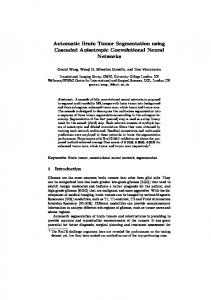
2(d) and 3(d), present the final results of the proposed model.                                   

 

  



  

              First, applying the Gaussian filter to the input image with                                                          resumed in the block diagram of figure (1). First, we adopt the Modified Fuzzy C Means algorithm. Eventually, we use the Adaptive Diffusion Flow Active Contours [6] [12] defined                                             

  

                                                                        inhomogeneities or noisy images. Although, if we add firstly the Modified Fuzzy C Means algorithm, we can obtain more efficient method which can provide better results.                   

                                                   

      

  

 

 

 

  





  





  





  





  





  





                                                                            in the table (I), the results related to the figure (2) show                                                 sufficient and reliable one.

217

 

                      -d- Progression of the ADF level sets method, -e- final contour with the ADF              with ADF method, -h- Progression of the ADF level sets, -i- final contour      

          

 

 

 

  





  





  





  





  





   







                                                                             [4] O. Mellina-Gottardo N. Paragios and V. Ramesh, “Gradient vector flow                                       flow fast geometric active contours,” in             [6] Yunde Jia Yuwei Wu and Yuanquan Wang, “Adaptive diffusion flow               [7] Rafika Harrabi and Ezzeddine Ben Braiek, “Colour image segmentation using the second order statistics and a modified fuzzy c-means tech Scientific Research and Essays       [8] C. Xu and J. L. Prince, “Snakes, shapes, and gradient vector flow,”                                                                                             [12] Yunde Jia Yuwei Wu and Yuanquan Wang, “Adaptive diffusion flow                                    

 

          fied Fuzzy C Means which combines the Adaptive Diffusion                                                  database in order to confirm the model performances. In a            

218