Hindawi Publishing Corporation Mathematical Problems in Engineering Volume 2013, Article ID 316546, 10 pages http://dx.doi.org/10.1155/2013/316546
Research Article Brain MR Image Segmentation Based on an Adaptive Combination of Global and Local Fuzzy Energy Wenchao Cui,1,2 Yi Wang,1 Tao Lei,1,3 Yangyu Fan,1 and Yan Feng1 1
School of Electronics and Information, Northwestern Polytechnical University, Xi’an 710072, China College of Science, China Three Gorges University, Yichang 443002, China 3 School of Electronic and Information Engineering, Lanzhou Jiaotong University, Lanzhou 730070, China 2
Correspondence should be addressed to Yi Wang;
[email protected] Received 17 May 2013; Accepted 19 October 2013 Academic Editor: Dane Quinn Copyright © 2013 Wenchao Cui et al. This is an open access article distributed under the Creative Commons Attribution License, which permits unrestricted use, distribution, and reproduction in any medium, provided the original work is properly cited. This paper presents a novel fuzzy algorithm for segmentation of brain MR images and simultaneous estimation of intensity inhomogeneity. The proposed algorithm defines an objective function including a local fuzzy energy and a global fuzzy energy. Based on the assumption that the local image intensities belonging to each different tissue satisfy Gaussian distributions with different means, we derive the local fuzzy energy by utilizing maximum a posterior probability (MAP) and Bayes rule. The global fuzzy energy is defined by measuring the distance between the original image and the corresponding inhomogeneity-free image. We combine the global fuzzy energy with the local fuzzy energy using an adaptive weight function whose value varies with the local contrast of the image. This combination enables the proposed algorithm to address intensity inhomogeneity and to improve the accuracy of segmentation and its robustness to initialization. Besides, the proposed algorithm incorporates neighborhood spatial information into the membership function to reduce the impact of noise. Experimental results for synthetic and real images validate the desirable performances of the proposed algorithm.
1. Introduction Magnetic resonance imaging (MRI), compared to other medical imaging modalities, has many significant advantages, including high contrast among different soft tissues, relatively high spatial resolution across the entire field of view, and multispectral characteristics [1]. Thus, it has been widely used in both clinical practice and neuroscience research. For example, quantitative analysis of brain tissues, that is, white matter (WM), gray matter (GM), and cerebral spinal fluid (CSF) from brain MR images provides very helpful information for the study and the treatment of various pathologies such as Alzheimer disease, Parkinson, or Parkinson-related syndrome. Therefore, accurate segmentation of brain MR images is an essential and vital step. However, due to nonuniform magnetic field or susceptibility effects, brain MR images are usually corrupted by intensity inhomogeneity which is also referred to as the bias field and manifests itself as a smooth intensity variation across the image [2]. As a result, the intensities of the same tissue vary with the locations of the
tissue within the image. This may cause serious misclassification when intensity-based segmentation algorithms are used. Therefore, intensity inhomogeneity has been a challenging difficulty in the task of image segmentation. Among many available segmentation algorithms, fuzzy segmentation methods, especially the fuzzy c-means (FCM)based algorithms, have been broadly applied to brain MR image segmentation. Such a success chiefly attributes to the introduction of fuzziness for the belongingness of each image pixel [3]. This enables the clustering methods to retain more information from the original image than the crisp or hard segmentation methods [4]. Pham and Prince [4] proposed an adaptive FCM algorithm which incorporated a spatial penalty term into the objective function to enable the estimated membership functions to be spatially smoothed. Ahmed et al. [5] developed the bias-corrected FCM (BCFCM) algorithm which modified the objective function of the standard FCM algorithm to compensate for intensity inhomogeneity and to allow the labeling
2 of a pixel to be influenced by the labels in its immediate neighborhood. Liew and Yan [6] used a B-spline surface to model the bias field and incorporated the spatial continuity constraints into fuzzy clustering algorithm. Zhang and Chen [7] replaced the original Euclidean distance with a kernelinduced distance and supplemented the objective function with a spatial penalty term, which modeled the spatial continuity compensation. Incorporating spatial information into the membership function, Chuang et al. [8] proposed a modified FCM algorithm which was less sensitive to noise and yielded more homogeneous segmented regions. Recently, local intensity information has been taken into account to deal with intensity inhomogeneity in fuzzy segmentation methods. For example, Li et al. [9] proposed a fuzzy energy minimization method based on coherent local intensity clustering (CLIC) for simultaneous tissue classification and bias field estimation of MR images. This CLIC algorithm draws upon intensity means in local regions; therefore, it can be used to segment images with intensity inhomogeneity. However, global information is not taken into account in this model; as a result, this model is not robust to the parameters and also apt to suffer from misclassification for the pixels on the boundary especially in the regions with heavy level of intensity inhomogeneity [1]. Ji et al. [10] assumed that the local image data within each pixel’s neighborhood satisfied the Gaussian mixture model (GMM), and thus proposed the fuzzy local GMM (FLGMM) algorithm. Since this algorithm exploits local intensity means and variances, it produces more accurate segmentation results than several state-of-theart algorithms. Nevertheless, it has a nonconvex objective function, and hence could be easily trapped in a local minimum, resulting in an unsatisfactory segmentation [10]. In addition, for clustering-based image segmentation algorithm, spatial correlation is frequently used to reduce the impact of noise [3, 5–8]. However, both the CLIC algorithm and the FLGMM algorithm ignore the spatial information; thus, they are sensitive to noise to some extent. In this paper, in order to handle intensity inhomogeneity, we assume that the local image intensities belonging to each different tissue satisfy Gaussian distributions with different means, and then apply maximum a posteriori probability (MAP) and Bayes rule to derive a local fuzzy energy function in which the bias field accounting for intensity inhomogeneity acts as a variable. For the purpose of improving the accuracy of segmentation and alleviating the problems induced by the nonconvexity of the proposed local fuzzy energy function, we introduce a global fuzzy energy which is defined by measuring the distance between the original image and the corresponding inhomogeneity-free image. Moreover, these two energy functions are combined using an adaptive weight function whose value varies with the local contrast of the image. Besides, the proposed algorithm incorporates neighborhood spatial information into the membership function to reduce the impact of noise. Therefore, our proposed algorithm can effectively segment brain MR images with severe intensity inhomogeneity and noise. The remainder of this paper is organized as follows. Section 2 gives the image model for intensity inhomogeneity.
Mathematical Problems in Engineering In Section 3, we present the definition and minimization of the proposed fuzzy objective function in detail. We describe how to utilize neighborhood spatial information in Section 4. The implementation and experimental results are given in Section 5. The discussion on the setting of important parameters is given in Section 6. We end this paper by the conclusion in Section 7.
2. Image Model for Intensity Inhomogeneity Intensity inhomogeneity can be modeled as a multiplicative component of an observed image [2], as shown in the following: 𝐼 = 𝑏𝐽 + 𝑛,
(1)
where 𝐼 is the observed image, 𝑏 is an unknown bias field, 𝐽 is the inhomogeneity-free image or true image, and 𝑛 is the additive noise. A generally accepted assumption on the bias field 𝑏 is that it is smooth or slowly varying. Ideally, the intensity 𝐽 belonging to the 𝑖th tissue should take a specific value 𝑐𝑖 , which represents the measured physical property. The additive noise 𝑛 is assumed to be Gaussian noise with zero mean and variance 𝜎2 .
3. Our Proposed Objective Function The proposed objective function includes a local fuzzy energy and a global fuzzy energy, which are formulated by exploiting local intensity information and global intensity information, respectively. In this section, we will give a detailed description with respect to the definition and minimization of the objective function. 3.1. Local Fuzzy Energy. To effectively exploit information on local intensities, we need to characterize the distribution of local intensities via partition of neighborhood as in [11]. For each point 𝑦 in the image domain Ω, we consider a circular neighborhood with a small radius 𝑟, which is defined as 𝑂𝑦 = {𝑥 : |𝑥 − 𝑦| ≤ 𝑟}. The partition {Ω𝑖 }𝑁 𝑖=1 (𝑁 is the total number of segmented tissues) of the entire domain Ω induces a partition of the neighborhood 𝑂𝑦 ; that is, {𝑂𝑦 ∩ Ω𝑖 }𝑁 𝑖=1 forms a partition of 𝑂𝑦 . For a slowly varying bias field 𝑏, the values 𝑏(𝑥) for all 𝑥 in the circular neighborhood 𝑂𝑦 can be well approximated by its value 𝑏(𝑦) at the center of 𝑂𝑦 ; that is, 𝑏 (𝑥) ≈ 𝑏 (𝑦) ,
𝑥 ∈ 𝑂𝑦 .
(2)
Together with the aforementioned assumption with respect to the true image 𝐽 and the Gaussian noise 𝑛 in (1), we can describe the intensities 𝐼(𝑥) within subregion 𝑂𝑦 ∩ Ω𝑖 as a Gaussian distribution with mean 𝑏(𝑦) ⋅ 𝑐𝑖 and variance 𝜎2 . In other words, the probability density in subregion 𝑂𝑦 ∩ Ω𝑖 is 2
𝑝𝑖,𝑦 (𝐼 (𝑥)) =
(𝐼 (𝑥) − 𝑏 (𝑦) 𝑐𝑖 ) 1 ). exp(− √2𝜋𝜎 2𝜎2
(3)
Mathematical Problems in Engineering
3
Now, we consider the segmentation of the circular neighborhood 𝑂𝑦 based on the maximum a posteriori probability (MAP). Let 𝑝(𝑥 ∈ 𝑂𝑦 ∩ Ω𝑖 | 𝐼(𝑥)) be the a posteriori probability of the subregion 𝑂𝑦 ∩ Ω𝑖 given the neighborhood gray values 𝐼(𝑥). According to the Bayes rule,
𝑝 (𝐼 (𝑥) | 𝑥 ∈ 𝑂𝑦 ∩ Ω𝑖 ) 𝑝 (𝑥 ∈ 𝑂𝑦 ∩ Ω𝑖 ) 𝑝 (𝐼 (𝑥))
(4) ,
where 𝑝(𝐼(𝑥) | 𝑥 ∈ 𝑂𝑦 ∩ Ω𝑖 ) is the probability density in region 𝑂𝑦 ∩ Ω𝑖 , which is denoted by 𝑝𝑖,𝑦 (𝐼(𝑥)) in (3). 𝑝(𝑥 ∈ 𝑂𝑦 ∩ Ω𝑖 ) is the a priori probability of the partition 𝑂𝑦 ∩ Ω𝑖 among all partitions of 𝑂𝑦 , which is usually set equal in all partitions [12]. The a priori probability 𝑝(𝐼(𝑥)) is independent of the choice of the region. Assuming that the pixels within each region are independent, the MAP can be achieved by finding the maximum of ∏𝑁 𝑖=1 ∏𝑥∈Ω𝑖 ∩𝑂𝑦 𝑝𝑖,𝑦 (𝐼(𝑥)). Taking a logarithm, the maximization can be converted to the minimization of the following energy: 𝑁
𝐸𝑦 = ∑ ∫
𝑖=1 𝑂𝑦 ∩Ω𝑖
𝑁
𝐸𝑦 = ∑ ∫ −𝑢𝑖𝑚 (𝑥) 𝜔 (𝑥 − 𝑦) log 𝑝𝑖,𝑦 (𝐼 (𝑥)) 𝑑𝑥, 𝑖=1 Ω
𝑝 (𝑥 ∈ 𝑂𝑦 ∩ Ω𝑖 | 𝐼 (𝑥)) =
where 𝜏 is the standard deviation of the Gaussian kernel and 𝑎 is a constant to normalize the Gaussian kernel. The energy function 𝐸𝑦 in (7) can be rewritten as
− log 𝑝𝑖,𝑦 (𝐼 (𝑥)) 𝑑𝑥.
(5)
Now, we introduce the fuzzy membership function 𝑢𝑖 (𝑥) into the above energy. Since 𝑢𝑖 (𝑥) represents the probability of pixel 𝑥 belonging to region Ω𝑖 such that 𝑢𝑖 (𝑥) = 0 for 𝑥 ∉ Ω𝑖 , we can rewrite (5) as 𝑁
𝐸𝑦 = ∑ ∫ −𝑢𝑖𝑚 (𝑥) log 𝑝𝑖,𝑦 (𝐼 (𝑥)) 𝑑𝑥, 𝑖=1 𝑂𝑦
as 𝜔(𝑥 − 𝑦) = 0 for 𝑥 ∉ 𝑂𝑦 . The ultimate goal is to minimize 𝐸𝑦 for all the center points 𝑦 in the image domain Ω, which directs us to define the following double integral energy functional as our proposed local fuzzy energy: 𝐸𝐿 = ∫ 𝐸𝑦 𝑑𝑦 Ω
𝑁
= ∫ (∑ ∫ −𝑢𝑖𝑚 (𝑥) 𝜔 (𝑥 − 𝑦) log 𝑝𝑖,𝑦 (𝐼 (𝑥)) 𝑑𝑥) 𝑑𝑦. Ω
𝑖=1 Ω
(10) 3.2. Global Fuzzy Energy. Although many algorithms, such as fuzzy segmentation method [10] and active contour models [11, 13–16] have utilized only the local intensity information to successfully segment images with intensity inhomogeneity, a common drawback for these algorithms is that they have a nonconvex energy function and thus are easy to result in local optima. To avoid unsatisfying segmentation results led by bad initial conditions, a usual settlement is to incorporate the global intensity information [17–22]. In this paper, we measure the distance between the original image and the corresponding inhomogeneity-free image as the global energy function to be minimized. Our proposed global fuzzy energy is defined as 𝑁
(6)
2 𝐸𝐺 = ∫ (∑𝑢𝑖𝑚 (𝑥) 𝐼 (𝑥) − 𝑐𝑖 ) 𝑑𝑥, Ω
where 𝑚 is a weighting exponent on each fuzzy membership and determines the amount of fuzziness of the resulting classification. Next, we use a weighting function to impose spatial constraint as in [9, 13], we define the following objective function: 𝑁
𝐸𝑦 = ∑ ∫ −𝑢𝑖𝑚 (𝑥) 𝜔 (𝑥 − 𝑦) log 𝑝𝑖,𝑦 (𝐼 (𝑥)) 𝑑𝑥, 𝑖=1 𝑂𝑦
(7)
where 𝜔(𝑥 − 𝑦) is a nonnegative weighting function such that 𝜔(𝑥 − 𝑦) = 0 for |𝑥 − 𝑦| > 𝑟 and ∫𝑂𝑦 𝜔(𝑥 − 𝑦) 𝑑𝑥 = 1. Although the choice of the weighting function is flexible, it is preferable to use a weighting function 𝜔(𝑥 − 𝑦) such that larger weights are assigned to the data 𝐼(𝑥) for 𝑥 closer to the center 𝑦 of the neighborhood 𝑂𝑦 . In this paper, the weighting function 𝜔 is chosen as a truncated Gaussian kernel as follows: { 1 𝑒−|𝑑| /2𝜏 , 𝜔 (𝑑) = { 𝑎 {0, 2
2
|𝑑| ≤ 𝑟, else,
(11)
𝑖=1
where 𝑐𝑖 is the constant value of intensity 𝐽 belonging to the 𝑖th tissue in the inhomogeneity-free image. Because 𝑢𝑖 (𝑥) (0 ≤ 𝑢𝑖 (𝑥) ≤ 1) represents the probability that pixel 𝐼(𝑥) belongs to the 𝑖th tissue, the distance at location 𝑥 between the original image and the corresponding inhomogeneity-free image should be a weighted summation, that is, 𝑑(𝑥) = 2 𝑚 ∑𝑁 𝑖=1 𝑢𝑖 (𝑥)|𝐼(𝑥) − 𝑐𝑖 | . Adding up the distance 𝑑(𝑥) for all 𝑥 in the whole image domain Ω, we can get the expression as presented in (11). 3.3. Definition of the Objective Function. We combine the local fuzzy energy 𝐸𝐿 with the global fuzzy energy 𝐸𝐺, and thus obtain the proposed objective function as follows: 𝑁
2 𝐸 = 𝛽 ∫ (∑𝑢𝑖𝑚 (𝑥) 𝐼 (𝑥) − 𝑐𝑖 ) 𝑑𝑥 Ω
𝑖=1
𝑁
+ ∫ (∑ ∫ −𝑢𝑖𝑚 (𝑥) 𝜔 (𝑥 − 𝑦) log 𝑝𝑖,𝑦 (𝐼 (𝑥)) 𝑑𝑥) 𝑑𝑦, Ω
(8)
(9)
𝑖=1 Ω
(12) where 𝛽 (0 ≤ 𝛽 ≤ 1) is the weight of the global fuzzy term.
4
Mathematical Problems in Engineering
Generally speaking, in regions far away from the desired boundary of objects (i.e., tissues) where the intensities vary slowly and appear approximately homogeneous, the probability density 𝑝𝑖,𝑦 (𝐼(𝑥))(𝑥 ∈ 𝑂𝑦 ∩ Ω𝑖 ) for different cluster 𝑖 in local region 𝑂𝑦 is almost the same, thus the estimated membership functions by minimizing the energy 𝐸𝑦 in (7) will be approximately equal to each other; that is, the segmentation result is very “fuzzy”. This will result in inaccuracy after defuzzification. However, the global fuzzy energy in (11) is very appropriate to segment piecewise homogeneous regions because it is similar to the standard FCM objective function. Hence, we should increase the weight of the global fuzzy term to reduce the “fuzzy” degree of the estimated membership functions. On the contrary, in regions close to the desired boundary of objects, the probability density 𝑝𝑖,𝑦 (𝐼(𝑥)) can precisely reflect the difference of distributions for different tissues and may have a large deviation if we introduce the global fuzzy term redundantly. Thus, we need to reduce the weight of the global fuzzy term in such regions. Based on the above discussion, we should choose a weight function for 𝛽 that varies dynamically with the locations of the image instead of a constant value. Therefore, we refer to [19–22] and define the weight function 𝛽 as follows: 𝛽 (𝑥) = 𝛾 ⋅ mean (LCR𝑊 (𝑥)) ⋅ (1 − LCR𝑊 (𝑥))
(𝐼𝐿 max − 𝐼𝐿 min ) , 𝐼𝑔
𝑁
2 𝐹 = 𝛽 ∫ (∑𝑢𝑖𝑚 (𝑥) 𝐼 (𝑥) − 𝑐𝑖 ) 𝑑𝑥 Ω
𝑖=1
𝑁
+ ∫ (∑ ∫ −𝑢𝑖𝑚 (𝑥) 𝜔 (𝑥 − 𝑦) log 𝑝𝑖,𝑦 (𝐼 (𝑥)) 𝑑𝑥) 𝑑𝑦 Ω
𝑖=1 Ω 𝑁
+ 𝜆 (1 − ∑𝑢𝑖 (𝑥)) . 𝑖=1
(15) Taking the derivative of 𝐹 with respect to 𝑢𝑖 (𝑥) and setting the result to zero, we have, for 𝑚 > 1, [
𝜕𝐹 2 = 𝛽𝑚𝑢𝑖𝑚−1 (𝑥) 𝐼 (𝑥) − 𝑐𝑖 𝜕𝑢𝑖 (𝑥) + ∫ −𝑚𝑢𝑖𝑚−1 (𝑥) 𝜔 (𝑥 − 𝑦)
(14)
where 𝑊 defines the size of the local square window centered on 𝑥. we set 𝑊 = 5 for all experiments in this paper. 𝐼𝐿 max and 𝐼𝐿 min are the maximum and minimum of intensities within this local window, respectively. 𝐼𝑔 represents the total intensity levels of the image, for example, 𝐼𝑔 = 255 for gray image. In the above weight function (13), mean (LCR𝑊(𝑥)) is the average value of LCR𝑊(𝑥) over the whole image and it can reflect the overall contrast information of the image. For an image with a higher overall contrast, the background and foreground may be more clearly classified on the whole; thus, a bigger weight proportional to mean (LCRW (x)) should be chosen for the global fuzzy term. (1 − LCR𝑊(𝑥)) can adjust the weight of global fuzzy term dynamically in all regions, making it smaller in regions with high local contrast and larger in regions with low local contrast.
(16)
Ω
× log 𝑝𝑖,𝑦 (𝐼 (𝑥)) 𝑑𝑦 − 𝜆]
𝑥 ∈ Ω, (13)
where 𝛾 is an adjustable parameter and LCR𝑊 denotes the local contrast ratio of the given image, which is defined as LCR𝑊 (𝑥) =
The energy 𝐸 is subject to the constraint ∑𝑁 𝑖=1 𝑢𝑖 (𝑥) = 1. Thus, this constrained optimization will be solved using one Lagrange multiplier as follows:
𝑢𝑖 (𝑥)=𝑢𝑖∗ (𝑥)
= 0.
Solving for 𝑢𝑖∗ (𝑥), we have 𝑢𝑖∗ (𝑥) 1/(𝑚−1)
𝜆
=( ) 2 𝛽𝑚𝐼 (𝑥)−𝑐𝑖 +∫Ω −𝑚𝜔 (𝑥−𝑦) log 𝑝𝑖,𝑦 (𝐼 (𝑥)) 𝑑𝑦
. (17)
Since ∑𝑁 𝐾=1 𝑢𝑘 (𝑥) = 1 for all 𝑥, we have 𝑁
1/(𝑚−1)
𝜆
) ∑( 2 𝛽𝑚𝐼 (𝑥)−𝑐𝑘 +∫Ω −𝑚𝜔 (𝑥 − 𝑦) log 𝑝𝑘,𝑦 (𝐼 (𝑥)) 𝑑𝑦
𝑘=1
= 1, (18) or 𝜆=𝑚 𝑁
2 × (( ∑ ( (𝛽𝐼 (𝑥) − 𝑐𝑘 𝑘=1
3.4. Minimization of the Objective Function. Our proposed objective function 𝐸 in (12) can be minimized in a fashion similar to the standard FCM algorithm. Taking the first derivatives of 𝐸 with respect to 𝑢𝑖 (𝑥), 𝑏(𝑦), 𝑐𝑖 and 𝜎, and setting them to zero results in four necessary but not sufficient conditions for 𝐸 to be at a local extremum. In this subsection, we will derive these four conditions.
𝑚−1 −1 −1 1/(𝑚−1)
+∫ −𝜔 (𝑥−𝑦)log 𝑝𝑘,𝑦 (𝐼 (𝑥)) 𝑑𝑦) ) Ω
) ). (19)
Substituting (3) and (19) into (17), the zero-gradient condition for the membership functions can be rewritten as
Mathematical Problems in Engineering
𝑢𝑖∗ (𝑥) =
5
1 . 1/(𝑚−1) 2 2 𝛽𝐼 (𝑥) − 𝑐𝑖 + ∫Ω 𝜔 (𝑥 − 𝑦) (log (√2𝜋𝜎) + (𝐼 (𝑥) − 𝑏 (𝑦) 𝑐𝑖 ) /2𝜎2 ) 𝑑𝑦 𝑁 ) ∑𝑘=1 ( 2 2 𝛽𝐼 (𝑥) − 𝑐𝑘 + ∫Ω 𝜔 (𝑥 − 𝑦) (log (√2𝜋𝜎) + (𝐼 (𝑥) − 𝑏 (𝑦) 𝑐𝑘 ) /2𝜎2 ) 𝑑𝑦
In a similar way, taking the derivative of 𝐹 with respect to 𝑏(𝑦) and setting the result to zero, we have
(20)
Likewise, taking the derivative of 𝐹 with respect to 𝑐𝑖 and 𝜎 and setting the results to zero, we have [2𝛽 ∫ 𝑢𝑖𝑚 (𝑥) (𝐼 (𝑥) − 𝑐𝑖 ) (−1) 𝑑𝑥 Ω
𝑁
+ ∫ ∫ 𝑢𝑖𝑚 (𝑥) 𝜔 (𝑥 − 𝑦)
[∑ ∫ 𝑢𝑖𝑚 (𝑥) 𝜔 (𝑥 − 𝑦)
Ω
𝑖=1 Ω
(21)
× (𝐼 (𝑥) − 𝑏 (𝑦) 𝑐𝑖 ) (−𝑐𝑖 ) 𝑑𝑥]
×
= 0.
(𝐼 (𝑥) − 𝑏 (𝑦) 𝑐𝑖 ) (−𝑏 (𝑦)) 𝑑𝑥𝑑𝑦] = 0, 𝜎2 𝑐 =𝑐∗ 𝑖
𝑏(𝑦)=𝑏∗ (𝑦)
𝑖
(23) 𝑁
[∑ ∫ ∫ 𝑢𝑖𝑚 (𝑥) 𝜔 (𝑥 − 𝑦)
Solving for 𝑏∗ (𝑦), we have
∗
𝑏 (𝑦) =
𝑖=1
𝑚 ∑𝑁 𝑖=1 ∫Ω 𝑢𝑖 (𝑥) 𝜔 (𝑥 − 𝑦) 𝐼 (𝑥) 𝑐𝑖 𝑑𝑥 𝑚 2 ∑𝑁 𝑖=1 ∫Ω 𝑢𝑖 (𝑥) 𝜔 (𝑥 − 𝑦) 𝑐𝑖 𝑑𝑥
𝑐𝑖∗
=
Ω
(24) 2
2
× (𝜎 − (𝐼 (𝑥) − 𝑏 (𝑦) 𝑐𝑖 ) ) 𝑑𝑥𝑑𝑦] (22)
= 0. 𝜎=𝜎∗
Solving for 𝑐𝑖 and 𝜎, we have
2𝛽 ∫Ω 𝑢𝑖𝑚 (𝑥) 𝐼 (𝑥) 𝑑𝑥 + ∫ ∫Ω 𝑢𝑖𝑚 (𝑥) 𝜔 (𝑥 − 𝑦) 𝐼 (𝑥) 𝑏 (𝑦) (1/𝜎2 ) 𝑑𝑥 𝑑𝑦 2𝛽 ∫Ω 𝑢𝑖𝑚 (𝑥) 𝑑𝑥 + ∫ ∫Ω 𝑢𝑖𝑚 (𝑥) 𝜔 (𝑥 − 𝑦) 𝑏2 (𝑦) (1/𝜎2 ) 𝑑𝑥 𝑑𝑦
,
(25)
2
𝜎∗ = √
𝑚 ∑𝑁 𝑖=1 ∫ ∫Ω 𝑢𝑖 (𝑥) 𝜔 (𝑥 − 𝑦) (𝐼 (𝑥) − 𝑏 (𝑦) 𝑐𝑖 ) 𝑑𝑥 𝑑𝑦 𝑚 ∑𝑁 𝑖=1 ∫ ∫Ω 𝑢𝑖 (𝑥) 𝜔 (𝑥 − 𝑦) 𝑑𝑥 𝑑𝑦
4. Exploiting Spatial Information One of the important characteristics of an image is that neighborhood pixels are highly correlated. In other words, these neighborhood pixels possess similar intensity, and the probability that they belong to the same cluster is great. This spatial relationship is important in clustering, but it is not utilized in a conventional FCM algorithm. To exploit the spatial information, we refer to [8] and define a spatial function as follows: ℎ𝑖 (𝑥) =
∑ 𝑢𝑖 (𝑦) ,
𝑦∈NB(𝑥)
(27)
where NB(𝑥) represents a square window centered on pixel 𝑥 in the spatial domain. A 5 × 5 window is used throughout this work. Just like the membership function, the spatial function ℎ𝑖 (𝑥) represents the probability that pixel 𝑥 belongs to the 𝑖th cluster. The spatial function of a pixel for a cluster is large if the majority of its neighborhood pixels belong to the same
.
(26)
cluster. The spatial function is incorporated into membership function as follows: 𝑢𝑖 (𝑥) =
𝑢𝑖 (𝑥) ℎ𝑖 (𝑥) . 𝑁 ∑𝑘=1 𝑢𝑘 (𝑥) ℎ𝑘 (𝑥)
(28)
In a homogeneous region, the spatial functions simply fortify the original membership, and the clustering result remains unchanged. However, for a noisy pixel, this formula reduces the weight of a noisy cluster by the labels of its neighborhood pixels. As a result, misclassified pixels from noisy regions or spurious blobs can easily be corrected.
5. Implementation and Experimental Results The proposed algorithm is a two-pass process at each iteration. The first pass is to calculate the corresponding variables 𝑢𝑖 (𝑥), 𝑏(𝑦), 𝑐𝑖 , and 𝜎. In the second pass, the membership function incorporated with the spatial information is updated and the resulting new membership function will be inserted
6
Mathematical Problems in Engineering
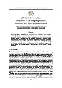
Figure 1: Segmentation results of the proposed algorithm on three synthetic images. Column 1: original images. Columns 2 and 3: intermediate results. Column 4: final results. Column 5: the estimated bias fields.
Figure 2: Comparison of segmentation results on two X-ray vessel images. Column 1: original images. Column 2: the BCFCM algorithm. Column 3: the sFCM algorithm. Column 4: the CLIC algorithm. Column 5: the proposed algorithm. Column 6: the estimated bias fields by the proposed algorithm.
into the next iteration. The detailed procedures can be summarized in the following steps. Step 1. Initialize the number of clusters 𝑁, membership function 𝑢𝑖 (𝑥), constant intensity value 𝑐𝑖 , and bias field 𝑏(𝑦). Step 2. Computing the weight function 𝛽 using (13). Step 3. Updating 𝜎, 𝑏(𝑦), 𝑢𝑖 (𝑥), and 𝑐𝑖 sequentially using (26), (22), (20), and (25), respectively. Step 4. Computing the new membership functions incorporated with spatial information using (28). Repeat Steps 3 and 4 till termination. The iteration is stopped when the maximum difference between two constant intensity values 𝑐𝑖 at two successive iterations is less than a threshold (e.g., 0.001). After the convergence, defuzzification is applied to assign each pixel to a specific cluster for which the membership is maximal.
In this paper, membership function 𝑢𝑖 (𝑥) and constant intensity value 𝑐𝑖 are initialized randomly at the intervals [0, 1] and [0, 255], respectively. Bias field 𝑏(𝑦) is initially equal to 1 for every pixel 𝑦. The parameters used in this paper are mostly set as the following default values: fuzzy exponent 𝑚 = 2, standard deviation of the Gaussian kernel 𝜏 = 4, and neighborhood radius of the Gaussian kernel 𝑟 = 14. Unless otherwise specified, the parameter 𝛾 is set to 0.005. 5.1. Segmentation of Synthetic Images. We first apply the proposed algorithm to three synthetic images to demonstrate its effectiveness. The original images shown in the first column of Figure 1 are corrupted by strong noise and intensity inhomogeneity. The parameters 𝛾 for these three images are set to 0.001. The intermediate segmentation results obtained by running the proposed algorithm for different numbers of iterations are shown in the second and third columns, and the final results obtained after the convergence of our
Mathematical Problems in Engineering
7
Figure 3: Comparison of segmentation results on two 3T brain MR images. Column 1: original images. Column 2: the BCFCM algorithm. Column 3: the sFCM algorithm. Column 4: the CLIC algorithm. Column 5: the proposed algorithm. Column 6: the estimated bias fields by the proposed algorithm.
Figure 4: Comparison of segmentation results on two simulated brain MR images. Column 1: original images. Column 2: the BCFCM algorithm. Column 3: the sFCM algorithm. Column 4: the CLIC algorithm. Column 5: the proposed algorithm. Column 6: ground truth.
algorithm are shown in the fourth column. The three images in the fifth column are the estimated bias fields. It is revealed from Figure 1 that the results gradually improve during the iterative segmentation process. In the final segmentation results, objects and background can be clearly differentiated despite of the impact of noise and intensity inhomogeneity. 5.2. Segmentation of Blood Vessel Images. In this subsection, we compare the proposed algorithm with the bias-corrected FCM (BCFCM) algorithm [5], the sFCM algorithm [8], and the CLIC algorithm [9] for blood vessel images. The images in the first column of Figure 2 are two Xray vessel images with noise and intensity inhomogeneity. In addition, some parts of the boundaries are quite weak. Our goal in this experiment is to segment the vessels from the inhomogeneous and noisy background. From the segmentation results shown in Figure 2, we can observe that both the BCFCM algorithm and the sFCM algorithm are based on the global intensity information and neither can address intensity inhomogeneity as well as the other two algorithms, that is, the CLIC algorithm and the proposed algorithm, which are based on local intensity information. Thus, they get rather unsatisfactory vessel segmentation results with some noisy spots, spurious blobs, and incomplete boundaries. By contrast with the CLIC algorithm, the proposed algorithm integrates the global and local intensity information and tries to exploit the neighborhood spatial information, and hence obtains desirable segmentation results with less spurious blobs. The
two images shown in the last column of Figure 2 are the estimated bias fields obtained by the proposed algorithm. 5.3. Segmentation of Brain MR Images. We also apply the aforementioned four algorithms to 3T brain MR images. The original images are also corrupted by intensity inhomogeneity and noise. The task of segmentation is to partition the brain MR images into four regions, that is, white matter (WM), gray matter (GM), cerebral spinal fluid (CSF), and background. The comparison of segmentation results obtained by these four algorithms is shown in Figure 3. Obviously, the BCFCM algorithm and the sFCM algorithm misclassify plentiful WM into GM in the vicinity of the skull, while the segmentation results of CLIC algorithm include a lot of noisy spots over the images. By contrast, our proposed algorithm gets fairly better segmentation with clear and correct classification of tissues. The estimated bias fields obtained by our proposed algorithm are shown in the sixth column of Figure 3. 5.4. Quantitative Comparison. To quantitatively compare the proposed algorithm with the above-mentioned other three algorithms, we use the T1-weighted simulated brain MR images with ground truth from Brain Web in the link http://www.bic.mni.mcgill.ca/brainweb/. The selected MR images contain 40% image intensity inhomogeneity and 3% noise. We set the parameter 𝛾 = 0.008 for these images. The original images and the segmentation results are shown
8
Mathematical Problems in Engineering 0.98
1
0.96 0.95 0.94 0.92
0.9 JS
JS
0.9 0.85
0.88 0.86
0.8
0.84 0.75 0.82 0.8
0.7 2
4
6
8 10 12 14 Neighborhood radius r
16
18
20
WM GM CSF
0
2
4
6 8 10 Standard deviation 𝜏
12
14
WM GM CSF
Figure 5: The JS values of the segmentation results obtained by using different parameter settings of the truncated Gaussian kernel.
Figure 6: Segmentation results obtained by the proposed algorithm with different parameter 𝛾 for images with less intensity inhomogeneity. Column 1: original images. Column 2: 𝛾 = 0.001. Column 3: 𝛾 = 0.005. Column 4: 𝛾 = 0.009.
in Figure 4. We adopt Jaccard similarity (JS) [2] as a measurement of the segmentation accuracy. The JS between two regions 𝑆1 and 𝑆2 is defined as the ratio between the areas of the intersection and the union of them, namely, JS(S1, S2) = |S1 ∩ S2|/|S1 ∪ S2|. We compute the JS between the segmented region 𝑆1 obtained by the algorithm and the corresponding region 𝑆2 given by the ground truth. The closer the JS value is to 1, the better the segmentation result. The resulting JS values for the four algorithms are listed in Table 1. It can be observed from both Figure 4 and Table 1 that the segmentation results of our proposed algorithm are more accurate than the other three algorithms. Meanwhile, we also compare the computation time of the four algorithms for the images in Figure 4. The CPU times are listed in Table 2, which are recorded from our experiments with Matlab programs run on a Dell Vostro 1450 notebook
with Intel Core i5 CPU, 2.5 GHz, 4 GB RAM, with Matlab R2010a on Windows 7. It is obvious that the BCFCM and sFCM algorithms have less time consumption, but they have lower segmentation accuracy. The CLIC algorithm and our proposed algorithm improve the segmentation accuracy at the cost of higher computational complexity. However, our algorithm accelerates the convergence of the iteration process by introducing the global fuzzy energy term; hence, it takes less CPU time than the CLIC algorithm.
6. Discussion In this paper, the truncated Gaussian kernel 𝜔 in (8) is used to determine the size of the local regions in which the proposed
Mathematical Problems in Engineering
9
Figure 7: Segmentation results obtained by the proposed algorithm with different parameter 𝛾 for images with strong intensity inhomogeneity. Column 1: original images. Column 2: 𝛾 = 0.001. Column 3: 𝛾 = 0.005. Column 4: 𝛾 = 0.009. Table 1: Comparison of the JS values of the segmentation results obtained by the four algorithms. Image
Tissue WM GM CSF WM GM CSF
Brain 1
Brain 2
BCFCM 0.9042 0.8433 0.8337 0.8561 0.8260 0.7938
Table 2: CPU time (seconds) comparison for the four algorithms. Image Brain 1 Brain 2
BCFCM 0.8268 0.7176
sFCM 0.6552 0.4992
CLIC 24.2894 21.2317
Proposed algorithm 11.0917 9.9841
local fuzzy energy is defined. Its two parameters, neighborhood radius 𝑟, and standard deviation 𝜏, can influence the segmentation accuracy to some extent. Figure 5 shows the JS values of the segmentation results with different parameter settings. The original image is obtained from Brain Web. The left figure shows the influence of the radius 𝑟 while the right figure shows the influence of the standard deviation 𝜏. It is clear that when 𝑟 > 8 or 𝜏 > 3, the JS values of WM, GM, and CSF remain stable on the whole. However, the time consumption would have a significant increase with the increase of the size of neighborhood radius. Considering the segmentation accuracy and the time consumption of the algorithm, we suggest that 9 ≤ 𝑟 ≤ 17 and 3 ≤ 𝜏 ≤ 6. In our experiments, we set 𝑟 = 14 and 𝜏 = 4 for all test images. As an adjustable variable of the weight function 𝛽, the parameter 𝛾 plays an important role to control the weight of the global and local fuzzy energy in our proposed objective function. Its value is typically selected from 0.001 to 0.01. If intensity inhomogeneity in the given image is severe, a value approximate to 0.001 should be chosen so that the local fuzzy energy is dominant. Otherwise, a bigger
sFCM 0.9168 0.8629 0.8491 0.8674 0.8387 0.8035
CLIC 0.9361 0.8985 0.8543 0.8683 0.8331 0.8184
Proposed algorithm 0.9562 0.9133 0.8958 0.9430 0.9098 0.8274
value close to 0.01 should be chosen. We first illustrate the effect of this parameter for the images with less intensity inhomogeneity. The original images are shown in the first column of Figure 6. The segmentation results obtained by our proposed algorithm with different 𝛾 are displayed from the second to fourth column of Figure 6. It can be seen that 𝛾 = 0.009 is more appropriate for this type of images. In addition, Figure 7 shows the segmentation results for images with strong intensity inhomogeneity using different 𝛾. It can be observed from the second to fourth column of Figure 7 that the segmentation results become more unsatisfactory with the increase of 𝛾. Therefore, we should choose the smaller 𝛾 for images with severe intensity inhomogeneity.
7. Conclusion In this paper, we have proposed a global and local fuzzy energy based algorithm for simultaneous segmentation and bias field estimation of images with different imaging modalities. The global fuzzy energy aims to minimize the distance between the original image and the corresponding inhomogeneity-free image. The local fuzzy energy is defined by using local intensity statistics and MAP and Bayes rule. These two fuzzy energy terms are combined using an adaptive weight function which depends on the local contrast of the image. This enables the proposed algorithm not only to address intensity inhomogeneity effectively but also to improve the accuracy of segmentation and its robustness
10 to initialization. Moreover, we utilize neighborhood spatial information to update the membership function in order to reduce the impact of noise. Comparisons with other approaches demonstrate the superior performance of the proposed algorithm.
Acknowledgments This work was supported by the National Natural Science Foundation of China (60903127, 61202314), the NPU Foundation for Fundamental Research (JCY20130130), “Top Paper” Project (13GH013308), and Ao-Xiang Star Project (11GH0315) at the Northwestern Polytechnical University, Xi’an, Shannxi, China.
References [1] Z.-X. Ji, Q. Chen, Q.-S. Sun, D.-S. Xia, and P.-A. Heng, “MR image segmentation and bias field estimation using coherent local and global intensity clustering,” in Proceedings of the 7th International Conference on Fuzzy Systems and Knowledge Discovery (FSKD ’10), vol. 2, pp. 578–582, IEEE Press, August 2010. [2] U. Vovk, F. Pernuˇs, and B. Likar, “A review of methods for correction of intensity inhomogeneity in MRI,” IEEE Transactions on Medical Imaging, vol. 26, no. 3, pp. 405–421, 2007. [3] S. Chen and D. Zhang, “Robust image segmentation using FCM with spatial constraints based on new kernel-induced distance measure,” IEEE Transactions on Systems, Man, and Cybernetics B, vol. 34, no. 4, pp. 1907–1916, 2004. [4] D. L. Pham and J. L. Prince, “An adaptive fuzzy C-means algorithm for image segmentation in the presence of intensity inhomogeneities,” Pattern Recognition Letters, vol. 20, no. 1, pp. 57–68, 1999. [5] M. N. Ahmed, S. M. Yamany, N. Mohamed, A. A. Farag, and T. Moriarty, “A modified fuzzy C-means algorithm for bias field estimation and segmentation of MRI data,” IEEE Transactions on Medical Imaging, vol. 21, no. 3, pp. 193–199, 2002. [6] A. W.-C. Liew and H. Yan, “An adaptive spatial fuzzy clustering algorithm for 3-D MR image segmentation,” IEEE Transactions on Medical Imaging, vol. 22, no. 9, pp. 1063–1075, 2003. [7] D.-Q. Zhang and S.-C. Chen, “A novel kernelized fuzzy C-means algorithm with application in medical image segmentation,” Artificial Intelligence in Medicine, vol. 32, no. 1, pp. 37–50, 2004. [8] K. Chuang, H. Tzeng, S. Chen, J. Wu, and T. Chen, “Fuzzy cmeans clustering with spatial information for image segmentation,” Computerized Medical Imaging and Graphics, vol. 30, no. 1, pp. 9–15, 2006. [9] C. Li, C. Xu, A. Anderson, and J. Gore, “MRI tissue classification and bias field estimation based on coherent local intensity clustering: a unified energy minimization framework,” in Proceedings of the 21st International Conference on Information Processing in Medical Imaging,, vol. 5636 of Lecture Notes in Computer Science, pp. 288–299, Springer, 2009. [10] Z. Ji, Y. Xia, Q. Sun, Q. Chen, D. Xia, and D. Feng, “Fuzzy local Gaussian mixture model for brain MR image segmentation,” IEEE Transactions on Information Technology in Biomedicine, vol. 16, no. 3, pp. 339–347, 2012. [11] L. Wang, L. He, A. Mishra, and C. Li, “Active contours driven by local Gaussian distribution fitting energy,” Signal Processing, vol. 89, no. 12, pp. 2435–2447, 2009.
Mathematical Problems in Engineering [12] N. Paragios and R. Deriche, “Geodesic active regions and level set methods for supervised texture segmentation,” International Journal of Computer Vision, vol. 46, no. 3, pp. 223–247, 2002. [13] C. Li, C.-Y. Kao, J. C. Gore, and Z. Ding, “Minimization of region-scalable fitting energy for image segmentation,” IEEE Transactions on Image Processing, vol. 17, no. 10, pp. 1940–1949, 2008. [14] C. Li, R. Huang, Z. Ding, J. C. Gatenby, D. N. Metaxas, and J. C. Gore, “A level set method for image segmentation in the presence of intensity inhomogeneities with application to MRI,” IEEE Transactions on Image Processing, vol. 20, no. 7, pp. 2007– 2016, 2011. [15] Y. Chen, J. Zhang, and J. Macione, “An improved level set method for brain MR images segmentation and bias correction,” Computerized Medical Imaging and Graphics, vol. 33, no. 7, pp. 510–519, 2009. [16] L. Wang, Y. Chen, X. Pan, X. Hong, and D. Xia, “Level set segmentation of brain magnetic resonance images based on local Gaussian distribution fitting energy,” Journal of Neuroscience Methods, vol. 188, no. 2, pp. 316–325, 2010. [17] L. Wang, C. Li, Q. Sun, D. Xia, and C.-Y. Kao, “Active contours driven by local and global intensity fitting energy with application to brain MR image segmentation,” Computerized Medical Imaging and Graphics, vol. 33, no. 7, pp. 520–531, 2009. [18] K.-K. Shyu, V.-T. Pham, T.-T. Tran, and P.-L. Lee, “Global and local fuzzy energy-based active contours for image segmentation,” Nonlinear Dynamics, vol. 67, no. 2, pp. 1559–1578, 2012. [19] Y. Yu, C. Zhang, Y. Wei, and X. Li, “Active contour method combining local fitting energy and global fitting energy dynamically,” in Proceedings of the International Conference on Medical Biometrics, vol. 6165 of Lecture Notes in Computer Science, pp. 163–172, Springer, 2010. [20] Y. Yang and B. Wu, “Convex image segmentation model based on local and global intensity fitting energy and split Bregman method,” Journal of Applied Mathematics, vol. 2012, Article ID 692589, 16 pages, 2012. [21] B. Wu and Y. Yang, “Local- and global-statistics-based active contour model for image segmentation,” Mathematical Problems in Engineering, vol. 2012, Article ID 791958, 16 pages, 2012. [22] Y. Yang and B. Wu, “Split Bregman method for minimization of improved active contour model combining local and global information dynamically,” Journal of Mathematical Analysis and Applications, vol. 389, no. 1, pp. 351–366, 2012.
Advances in
Operations Research Hindawi Publishing Corporation http://www.hindawi.com
Volume 2014
Advances in
Decision Sciences Hindawi Publishing Corporation http://www.hindawi.com
Volume 2014
Journal of
Applied Mathematics
Algebra
Hindawi Publishing Corporation http://www.hindawi.com
Hindawi Publishing Corporation http://www.hindawi.com
Volume 2014
Journal of
Probability and Statistics Volume 2014
The Scientific World Journal Hindawi Publishing Corporation http://www.hindawi.com
Hindawi Publishing Corporation http://www.hindawi.com
Volume 2014
International Journal of
Differential Equations Hindawi Publishing Corporation http://www.hindawi.com
Volume 2014
Volume 2014
Submit your manuscripts at http://www.hindawi.com International Journal of
Advances in
Combinatorics Hindawi Publishing Corporation http://www.hindawi.com
Mathematical Physics Hindawi Publishing Corporation http://www.hindawi.com
Volume 2014
Journal of
Complex Analysis Hindawi Publishing Corporation http://www.hindawi.com
Volume 2014
International Journal of Mathematics and Mathematical Sciences
Mathematical Problems in Engineering
Journal of
Mathematics Hindawi Publishing Corporation http://www.hindawi.com
Volume 2014
Hindawi Publishing Corporation http://www.hindawi.com
Volume 2014
Volume 2014
Hindawi Publishing Corporation http://www.hindawi.com
Volume 2014
Discrete Mathematics
Journal of
Volume 2014
Hindawi Publishing Corporation http://www.hindawi.com
Discrete Dynamics in Nature and Society
Journal of
Function Spaces Hindawi Publishing Corporation http://www.hindawi.com
Abstract and Applied Analysis
Volume 2014
Hindawi Publishing Corporation http://www.hindawi.com
Volume 2014
Hindawi Publishing Corporation http://www.hindawi.com
Volume 2014
International Journal of
Journal of
Stochastic Analysis
Optimization
Hindawi Publishing Corporation http://www.hindawi.com
Hindawi Publishing Corporation http://www.hindawi.com
Volume 2014
Volume 2014