November 15, 2009 / Vol. 34, No. 22 / OPTICS LETTERS
3583
Automatic deconvolution of 4Pi-microscopy data with arbitrary phase Giuseppe Vicidomini, Stefan W. Hell, and Andreas Schönle* MPI for Biophysical Chemistry, Am Fassberg 11, 37077 Göttingen, Germany *Corresponding author:
[email protected] Received July 2, 2009; revised October 6, 2009; accepted October 9, 2009; posted October 29, 2009 (Doc. ID 113567); published November 13, 2009 We propose a maximum a posteriori-based method that solves an important practical problem in the deconvolution of 4Pi images by simultaneously delivering an estimate of both the object and the unknown phase. The method was tested in simulations and on data from both test samples and biological specimen. It generates object estimates that are free from interference artifacts and reliably recovers arbitrary relative phases. Based on vectorial focusing theory, our theoretical analysis allowed for a simple and efficient implementation of the algorithm. Taking several 4Pi images at different relative phases of the interfering beams is shown to improve the robustness of the approach. © 2009 Optical Society of America OCIS codes: 110.0180, 180.2520, 180.6900, 100.1455.
By using two opposing objective lenses, the family of 4Pi microscopes [1] fundamentally improves the axial resolution of fluorescence microscopes. In the socalled 4Pi type A arrangement, the spherical wavefronts created by focusing the excitation laser beam through both lenses are coherently combined in the focus while emission is collected incoherently through at least one of the lenses and usually focused through a pinhole by the tube lens. Its effective pointspread function (E-PSF) thus depends on the relative phase of the two beams at the common focus and features several narrow diffraction maxima leading to periodic artifacts that must be removed by image restoration [2]. This makes precise knowledge of the E-PSF heff essential, but is often not known a priori and has to be estimated in a step preluding the actual estimation of the specimen function f. To this end, different methods were proposed in the literature, but their successful implementation relies on particular hardware arrangements [3,4] or special abilities of the operator [5]. Here, we propose to eliminate this extra step of phase estimation from the restoration algorithm by employing a fully automated parametric blind deconvolution (PBD) [6] method based on a maximum a posteriori (MAP) approach that simultaneously estimates both the phase difference and the specimen function. The optical transfer function (OTF) of a 4Pi microscope features regions of weak transmission. Hell et al. [3] showed that these critical frequencies are transmitted much less efficiently for destructive than for constructive interference, rendering the deconvolution process more robust against noise in the latter case. It may therefore be advantageous to take a number of different images gk at different phase values k = + ␦k by imposing a known phase shift ␦k, with k = 1 , . . . , N␦ and ␦1 = 0. This so called phasediversity (PD) approach ensures that at least one of the exposures is close to the constructive case; however, by splitting the photons between the individual images, the signal-to-noise ratio (SNR) is reduced. To explore this possibility we use a general multi-image approach for the formulation of the problem in Baye0146-9592/09/223583-3/$15.00
sian terms that thus aims at maximizing the a posteriori probability of observing the specimen f and the phase , given a series of images g = 兵gk其, P共f, 兩g兲 = P共g兩f, 兲P共f兲P共兲/P共g兲.
共1兲
P共g 兩 f , 兲 is the probability of observing g, while P共兲, P共g兲, and P共f兲 denote the a priori probability distributions for the phase, for the series of images, and for the specimen, respectively. We assume that, for any voxel n and any image k, the value gk共n兲 is a realization of an independent Poisson random variable with mean value 共Hkf兲共n兲, and therefore P共g兩f, 兲 = 兿 poi关gk共n兲兩共Hkf兲共n兲兴,
共2兲
k,n
where poi共g 兩 兲 = g exp共−兲 / g!, and we introduced the notation 共Hkf兲共n兲 for the discretization of the convolution heff共r , k兲 丢 f共r兲. Importantly, Hkf, can be easily calculated for given k by means of fast Fourier transforms (FFTs) with complexity O共N log N兲, N being the number of voxels. However, the writing Hk as a convolution operator implies a space-invariant E-PSF and thus is constant phase over the whole image. While this condition is not always met in life-cell imaging, it is a reasonable assumption in many practical cases, in particular when imaging fixed cells. In this case, constant phase can be achieved experimentally, e.g., by using the water-miscible TDE (2,2’Thidodiethanol) mounting medium [7] or optical phase compensation. In classical Tikhonov regularization P共f兲 is Gibbs distributed with a quadratic energy cost function exp共−储f储22兲, where the regularization parameter ⬎ 0 was set to 10−4 throughout the manuscript. If is uniformly distributed, then P共兲 = 1 / 2 for 0 艋 艋 2 and P共兲 = 0 elsewhere. Maximization of the function defined in Eq. (1) is then equivalent to minimizing its neglog given by © 2009 Optical Society of America
3584
OPTICS LETTERS / Vol. 34, No. 22 / November 15, 2009
J共f, 兩g兲 = 兺 兵共Hkf兲共n兲 − gk共n兲ln关共Hkf兲共n兲兴其 + 储f储22 ,
A2f = 关2I共E1*E2兲hCEF兴 丢 f
共14兲
k,n
共3兲 which was achieved using an alternating minimization method (AMM) [8]: For the lth step we have fl+1 = arg min J共f, l兩g兲,
共4兲
f艌0
l+1 = arg min J共fl+1, 兩g兲.
共5兲
To solve Eq. (4) under the nonnegativity constraint we use the so called split-gradient method (SGM) [9], which leads to the following iterative algorithm: fl,i+1 =
fl,i
兺 1 + fl,i k
冉
HkT
gk Hkfl,i
冊
,
i = 1, . . . ,NSGM , 共6兲
where 兺nheff共n , k兲 = 1 / N␦, quotient and product of vectors are voxel by voxel. Since Eq. (6) is dominated by FFT computation, each SGM iteration has complexity O共N log N兲. To solve Eq. (5) we adopt a steepest descent method (SDM):
l,i+1 = l,i − l,i共l,i兲,
共7兲
i = 1, . . . ,NSDM ,
The search direction 共l,i兲 is given by the gradient of J with respect to ,
共l,i兲 = ⵜ关J共fl+1, 兩g兲兴共l,i兲 =兺
k,n
再
冉
共Hk⬘ fl+1兲共n兲 1 −
gk共n兲 共Hkfl+1兲共n兲
冊冎
,
共8兲
where Hk⬘ f = Hkf / [see Eq. (10)], while the step size l,i is determined using the Armijo line-search method [10]. Thus each iteration of the SDM algorithm requires not only the evaluation of 共l,i兲 but also several calculation of J共fl+1 , 兩 g兲 for different values of owing to the line search. Fortunately the form of the 4Pi PSF allows avoiding recalculation of the convolutions, greatly speeding up the algorithm: The effective PSF of a 4Pi fluorescence microscope of type A using one-photon excitation is given by heff共r, k兲 = 兩E1共r兲 + exp共ik兲E2共r兲兩2hCEF共r兲,
are independent of k. A similar decomposition using five convolution operators can readily be derived for two-photon excitation. The operators are thus evaluated only during the first iteration, while successive iterations require only multiplications affording complexity O共N兲. As usual we chose f0,0 = const. While J is convex with respect to f at constant if the OTF is nonzero at the critical frequencies, it may have several local minima at different values of . We found that running the first SDM minimization for eight equidistant starting values 0,0 = m / 4, m = 0 , . . . , 7 is sufficient for overcoming this problem, and we achieved the fastest overall convergence to the estimates fE and E when initially choosing NSGM = NSDM = 5 and increasing this value to 10 after 50 iterations of the AMM algorithm. We validated our PBD method with synthetic data [Fig. 1(a)] assuming one-photon excitation and a confocal pinhole of 0.5 AU and using pairs of objectives with NAs of 1.46 (oil), 1.35 (glycerol), and 1.2 (water) corresponding to aperture angles ␣ of 74.5°, 68.5° and 64.1°. Figure 1 shows the results for the oil objectives. To assess a possible increase in robustness using a multi-imagebased approach we analyzed the Kullback–Leibler distance DKL共f , fE兲 [11] as a function of for both the single image (SI) and a PD 共N = 2 , ␦2 = 兲 mode [Figs. 1(e) and 1(f)]. While PD performs slightly better than taking a single image (at destructive phase, = , DKL is reduced by ⬇4%, 2%, and 1% for oil, glycerol, and water objectives, respectively), visual inspection of the resulting estimates indicates that the gain in quality is somewhat marginal. This small advantage has to be carefully weighed against possible motion artifacts introduced by sequential exposures with altering phase. The advantage of PD is reduced at low NA where inspection of the E-PSF shows that the dependence of the critical frequencies’ strength becomes negligible. Figure 1(f) shows that the phase
共9兲
where E1,2 denotes the counter-propagating focal fields, with E2共r兲 = ME1共Mr兲. The transformation matrix M accounts for the counterpropagation of the beams, and hCEF is the collection efficiency function. We can therefore write the operators Hk and Hk⬘ as linear combinations, Hkf = A0f + cos kA1f − sin kA2f,
共10兲
Hk⬘ f = − sin kA1f − cos kA2f,
共11兲
where the convolution operators A0f = 关共兩E1兩2 + 兩E2兩2兲hCEF兴 丢 f,
共12兲
A1f = 关2R共E1*E2兲hCEF兴 丢 f,
共13兲
Fig. 1. (Color online) (a) Test phantom and (b) example of a simulated image with = 7 / 8, NA 1.46 (oil), exc = 635 nm, em = 680 nm, pinhole 0.5 AU. (c) Deconvolution with known phase and (d) PBD (phase estimated, E = 2.66). (e) DKL共f , fE兲 and (f) E as functions of for SI and PD mode. Both graphs are obtained as the average of five different simulated images. For all simulations we fixed the total number of photons 兺k,ngk共n兲, resulting in a maximum of expected photons of ⬃50 共SNR⯝ 7 : 1兲 and ⬃25 共SNR⯝ 5 : 1兲 for SI and PD images, respectively.
November 15, 2009 / Vol. 34, No. 22 / OPTICS LETTERS
is reliably recovered for all possible values with no appreciable difference between the PD and SI approaches. Next, we deconvolved experimental data acquired with a 4Pi type A module [2] using two opposing objective lenses (HCS PL APO 100/ 1.46 OIL CORR, Leica Microsystem, Germany). Figure 2 shows recovery of the phase for fluorescent beads (100 nm Crimson beads, Molecular Probes, Ore., USA). The phase was varied by linearly changing the optical path length through one of the arms of the interferometric setup. Not surprisingly, our method recovers the phase reliably on this simplest of all possible samples. More importantly we therefore assessed the performance of PBD on images of biological relevance. We therefore applied it to data acquired during an investigation of the Golgi apparatus in Vero cells [7]. The images show GM 130 protein located in the cis-Golgi network immuno-labeled using Cy3 and embedded in TDE (Fig. 3). In this particular example the operator had tried to adjust to constructive interference. Deconvolving with this value leads to artifacts, while application of the PDB method results in significantly improved deconvolved data and estimates the actual phase at = 5.88. We thus demonstrated that the MAP-PBD approach is a suitable tool to estimate both the object function and the relative phase in 4Pi microscopy. We have tested the method on both synthetic and experimental data under realistic conditions. Taking several exposures at different phase values increases robustness against noise slightly but may introduce motion artifacts. The single-image mode can thus be recommended as a standard approach. While the phase estimate delivered by our method may also be made by an experienced user by assuming different values for and inspecting deconvolution results, this method is both unfit for automated data analysis and significantly slower, because it does not exploit the efficient decomposition of the 4Pi E-PSF used here. We therefore expect our approach to greatly benefit 4Pi users by providing a reproducible and re-
Fig. 2. (Color online) Bead images (exc = 635 nm, em = 680 nm, SNR⯝ 6 : 1) and object estimate in the case of constructive [(a), (b)] and destructive [(c), (d)] phase. (e) Robust estimation of arbitrary phases using the SI or PD 共N = 2 , ␦2 = 兲.
3585
Fig. 3. (Color online) (a) Axial 共xz兲 slice of a 3D stack of a Golgi apparatus (exc = 568 nm, em = 605 nm, SNR⯝ 7 : 1). (b) Deconvolved data without phase estimation ( is set to zero) and (c) with simultaneous phase estimation (estimated phase E = 5.88). Intensity profiles at site indicated by arrows (d). The residual sidelobes in the deconvolved data without phase estimation are removed by PBD. Scale bar, 0.5 m.
liable method to obtain optimal reconstruction results without the need for a possibly biased guess of the unknown phase parameter. Finally, we observe that the decomposition of the operator H in -dependent and -independent parts based on vectorial focusing theory introduced here is applicable to deconvolution algorithms with variable phase [5]. Future work will thus aim at extending our PDB approach to the case of unknown, variable phase in heterogeneous samples. We thank Roman Schmidt for help with the acquisition of the bead data and Marion Lang for providing the Golgi data. We also thank Alexander Egner and Johann Engelhardt for useful discussions. This work has been supported by the German Federal Ministry of Education and Research through the project INVERS. References 1. S. Hell and E. H. K. Stelzer, J. Opt. Soc. Am. A 9, 2159 (1992). 2. M. Nagorni and S. W. Hell, J. Opt. Soc. Am. A 18, 36 (2001). 3. S. W. Hell, C. M. Blanca, and J. Bewersdorf, Opt. Lett. 27, 888 (2002). 4. C. M. Blanca, J. Bewersdorf, and S. W. Hell, Opt. Commun. 206, 281 (2002). 5. D. Baddeley, C. Carl, and C. Cremer, Appl. Opt. 45, 7056 (2006). 6. J. Markham and J.-A. Conchello, J. Opt. Soc. Am. A 16, 2377 (1999). 7. M. Lang, T. Müller, J. Engelhardt, and S. W. Hell, Opt. Express 15, 2459 (2007). 8. J. C. Bezdek, R. J. Hathaway, R. E. Howard, C. A. Wilson, and M. P. Windham, J. Optim. Theory Appl. 54, 471 (1987). 9. G. Vicidomini, P. Boccacci, A. Diaspro, and M. Bertero, J. Microsc. 234, 47 (2009). 10. C. Kelley, Iterative Method for Optimization (SIAM, 1999), Vol. 18. 11. I. Csiszár, Ann. Stat. 19, 2032 (1991).