AUTOMATIC ESTIMATION OF VOICE SOURCE PARAMETERS Helmer Strik and Louis Boves University of Nijmegen, Dept. of Language and Speech P.O. Box 9103, 6500 HD Nijmegen, The Netherlands E-mail:
[email protected]
ABSTRACT
1. INTRODUCTION There is an increasing need for automatic techniques to extract the voice source parameters. Such a method is described in [1] and [2]. For natural speech (where the input is unknown) this method gave plausible results [1], while for synthetic speech (where the input is known) the parameters could be re-estimated with reasonable a accuracy [1,2]. At the moment we are testing and trying to improve this automatic method. In the proposed method the speech signal is inverse filtered, and the resulting estimate of glottal flow is parameterized by fitting a voice source model to the waveforms. Inverse filtering has been studied in detail; it is unlikely that the procedure can recover the input flow waveform exactly. Thus, is it necessary to know how a parametric model behaves when it is fitted to a corrupted flow signal. As a step in that direction we investigated the behaviour of one specific voice source model (i.e. the LFmodel [4]) in non-linear fit procedures. LF-pulses were fitted to flow signals to which several kinds of white and narrow band noise had been added. In the current article we investigate whether the performance of the fit depends on the way in which the LF-pulses are computed. We also study the difference between two classes of fit procedures, viz. simplex search and steepest descent algorithms.
2.1. Fit procedure In our work non-linear fit procedures are used to estimate LF-parameters from inverse filtered and therefore essentially noisy glottal flow signals [1,2]. The signal which results from inverse filtering is an estimate of differentiated glottal flow, denoted by dU g. Next, dUg is used to calculate the voice source parameters. For each pitch period an LF-model is fitted to dUg (see [2]). The fit procedure consists of three stages: » 1. initial estimate » 2. simplex search algorithm » 3. Levenberg-Marquardt algorithm Non-linear optimization algorithms require that an initial estimate is computed to start the procedure. The impact of the initial estimate on the final result is disc ussed in [2]. In the second stage of the fit procedure the s implex search algorithm of Nelder and Mead [3] is used. Of the several optimization algorithms that were tested the simplex search algorithm usually came closer to the global minimum than the gradient algorithms. Probab ly, discontinuities in the error function cause the gradient algorithms to get stuck in local minima more often than the simplex search algorithm. However, in the neighbour hood of a minimum, the simplex algorithm may do worse (see [3]). Therefore, the Levenberg-Marquardt algorithm (a gradient algorithm) is used after the simplex algorithm. In our work we have chosen the LF-model [4] for parameterization of dUg. In the fit procedure for each pitch period five LF-parameters are estimated, viz. E e, to, tp, te, and Ta (Fig. 1). The goal of the fit procedure is to
dUg
Voice source parameters can be estimated by fitting a voice source model to the glottal flow signal which is obtained by means of inverse filtering. In this pap er we investigate the behaviour of the LF-model in a number of non-linear parameter estimation procedures. It is concluded that (1) the parameter estimates are robust against additive (white and narrow band) noise in the flow waveforms, (2) simplex search algorithms perform better than steepest descent algorithms, provided that (3) the LF-pulse is generated with an algorithm that treats all parameters as real numbers.
2. METHOD
Ta to
tp
te
tc
-Ee Figure 1. The LF-model and the LF-parameters.
find the LF-parameters that minimize the difference between the LF-pulse and dUg. This is done by minimizing the RMS-error of the difference between the LF-pulse and dUg, i.e. the cost function is defined in the time dom ain. For all signals a sampling frequency of 10 kHz and an amplitude resolution of 12 bits were used.
Ee
%
2.2. Test method Tests were performed to evaluate in which way disturbances on dUg would affect the estimated parameters. LF-pulses were perturbated in a controlled way, and the LF-parameters of the disturbed signals were estimated by means of the fit procedure. The errors in the estim ated parameters were calculated in the following way: ERR(X) = 100%*abs(Xest - Xinp)/Xinp, for X = Ee ERR(Y) = abs(Yest - Yinp), for Y = to, tp, te, and Ta. Subsequently, the absolute values of the errors were averaged. In Figures 2 to 5 mean errors are shown. In the upper row are the mean errors in the estimations of Ee (unit: %), and in the middle and lower rows are the errors in the estimates of to, tp, te, and Ta (unit: µsec or msec). The effects of the perturbations cannot always be studied by a single, isolated LF-pulse. For instance, a formant ripple will be present in dU g when formant and bandwidth values are not estimated correctly. To calculate the first samples of dU g for the current pitch period, the speech signal that resulted from the previous e xcitation is used. This speech signal is dependent on th e amplitude and the shape of the previous flow pulse. Thus, the formant ripple at the beginning of the current pitch period will depend on the amplitude and the shape of the flow pulse in the previous pitch period. Therefore, we used sequences of three LF-pulses, and each time the voice source model was fitted to the (perturbated) pulse in the middle. Furthermore, 11 LF-pulses with different shapes were used. These 11 standard LFpulses will be called the basic pulses. The perturbated LFpulses will be called the test pulses.
3. TESTS 3.1. Quantization For the fit procedure an algorithm is needed that calculates an LF-pulse for each combination of the five LFparameters. Initially we used the algorithm of Lin described in [5]. In Lin’s algorithm Ee and tp can change continuously, but to and te are always rounded off towards the nearest integer (i.e. towards the nearest sample point). The consequence is that the error as a function of to or te is a step function. This is certainly problematic for gradient algorithms, but also for the simplex algorithm it often resulted in a false convergence to a local minimum. In order to make it possible to have non-integer estimates
to
te
shift (msec)
µsec
µsec
tp
Ta
shift (msec)
Figure 2. Mean and standard deviation of the error in the estimated LF-parameters for different values of shift. of to and te, we adapted Lin’s algorithm. In the adapted algorithm the analytic expression of the LF-model is used to calculate the LF-pulse in continuous time, and then the LF-pulse is sampled. With the new algorithm the fit procedure converged to the global minimum more often, and the resulting errors in the estimated parameters were considerably smaller. The new algorithm was investigated with test pulses generated by shifting the 11 basic pulses in steps of 0.02 msec (= 0.2 sample), from 0.0 to 0.1 msec (6 values for shift). The amplitude Ee was varied from -1025 to -1023 in steps of 0.2 (11 values for Ee). For the resulting 726 test pulses (11 x 6 x 11) a fit was done, and the estimated parameters were compared with the input values. In Fig. 2 for each value of shift the results for the 121 Ee values (11 x 11) were pooled, and mean and standard deviation were calculated. Similarly, In Fig. 3 for each value of Ee the 66 values of shift (11 x 6) were pooled, and again mean and standard deviation were calculat ed. In Fig. 2 and 3 can it be seen that for none of the values of shift and Ee the results deviate significantly. Also, no trend in the errors can be observed. Thus, it appea rs that with the proposed fit procedure and algorithm for calculation of the LF-pulse it is possible to get accurate estimates for all parameters.
Ee
to
te
Ee
Ee
%
µsec
µsec
tp
%
to
tp msec
Ta
te
Ta msec
Ee
SNR (dB)
SNR (dB)
Figure 3. Mean and standard deviation of the error in the estimated LF-parameters for different values
Figure 4. Meanerror in theestimated LFparameters for different values of SNR.
3.2. Noise
3.3. Formant ripple
In practice the voice source signal will always con tain noise. In this section we want to study the way in which noise affects the estimates. The noise present in the inverse filtered signal can come from many different sources, among which are noise sources at the glottis or in the vocal tract, background noise during the recordings, and quantization noise during A/D conversion. The amplitude and the spectrum of those noise sources m ay be difficult to establish. To simplify matters, we chose to use additive white noise. Although real noise may be different, it is still meaningful to test the influenc e of additive white noise on the estimated parameters. Noise with different amplitudes was added to the 11 basic pulses. The amplitudes were chosen such that the Signal-to-Noise Ratio (SNR) varied from 0 to 70 dB, in steps of 5 dB (15 SNR values). For calculation of the SNR the energy of the LF-pulse and the noise signal were integrated over the whole period. The LF-model was fitted to the 165 test pulses (11 x 15), and the mean errors for the estimated parameters were calculated (Fig. 4). It can be seen in Fig. 4 that the mean error increa ses with decreasing SNR. Of the time parameters the mean error in to is the largest. The explanation probably is that near to the signal generally changes more slowly than at other time points. Therefore, the noise has more effect on the fit in the neighbourhood of to, than on other places.
Errors in the estimation of formant (F m) and bandwidth (Bw) values used in inverse filtering will result in a formant ripple in dUg. In this section we focus on the effect that a formant ripple will have on the estim ated parameters. Test pulses were obtained by filtering the 11 basic pulses withfilter a consisting of 1 pole and 1 zero. The pole was kept fixed at the ’correct’ value of Fm and Bw, while the Fm and Bw values of the zero were varied. The error in F m (∆Fm) was varied between -20% and 20% of Fm, and the error in B w (∆Bw) between -50% and 100% of Bw. The results for Fm = 500 Hz and Bw = 80 Hz are shown in Fig. 5. The error in the estimates of the LF-parameters is smallest when there is no formant ripple (∆Fm = ∆Bw = 0), as was to be expected. For large values of ∆Fm and ∆Bw, and consequently a large ripple in the test pulse s, the errors in the estimates remain remarkably small. Probably, the explanation is that the best fit is determined for the whole period, and thus a local ripple does not need to have a drastic effect on the global fit. The mean error in T a is larger than the mean error in to, tp, and te. This is no surprise, as the formant ripple is most pronounced just after the main excitation. If Bw is not too large, the ripple will still be present at the beginning of the next pulse. This ripple can be problematic for the estimation of to, especially because the signal chan-
Ee
8
%
4. CONCLUSIONS
6 4 2 0 -100
-50
0
50
100
to
tp
250
µsec
200
150
100
150 100
50
50 0 -100
-50
0
50
100
te
150
0 -100
-50
0
50
100
50
100
Ta
500
µsec 400
100
300 200
50
100 0 -100
-50
0
50
∆Fm (Hz)
100
0 -100
-50
0
∆Fm (Hz)
Figure 5. Meanerror in theestimated LFparameters for different values of ∆Fm and ∆Bw (Fm = 500 Hz, Bw = 80 Hz). The different line types refer to different values of ∆Bw: -50% (solid), 0% (dashed), +50% (dotted), and +100% (dasheddotted).
ges relatively slowly around t o. This could be the reason why the mean errors in to are larger than the mean errors in tp and te. The experiment was repeated for other values of Fm and Bw. For formant values of 400 and 600 Hz and a bandwidth of 80 Hz the resulting errors were comparable with those in Fig. 5. But for higher formant values (in the range of the second and third formant) the errors were substantially smaller. The ripple caused by errors in the estimation of the second or third formant have higher frequencies and thus will be less problematic for the fit procedure than a ripple with a low frequency, caused by an error in the estimation of the first formant. Furth ermore, the bandwidth of higher formants will generally be larger than the bandwidth of the first formant, and the co rresponding ripple will damp out more quickly. This ripple will have less effect on the estimates of the following period.
In section 3.1. we showed that with the proposed method it is possible to get accurate estimations of time points that do not coincide with sample points. The algorithm used to calculate the LF-pulse proved to be very important, i.e. with an adapted version of Lin’s algo rithm [5] the errors in the estimations were considerably smaller than with the original version. The adapted algorithm is more time-consuming, but this is no problem for a fit procedure. The magnitude of the errors resulting from additive white noise increases with decreasing SNR. With a 12 bit quantization it is usually possible to have a SNR of at least 30 dB. If the SNR is higher than 30 dB the error in Ee is less than 0.5%, and the error in the time parameters is less than 0.02 msec (i.e. 0.2 sample). For most applications this is probably acceptable. Errors in the estimation of the first formant have more effect on the estimated parameters than errors in t he higher formants. For this reason, special attention should be given to the estimation of the first formant during inverse filtering. For the disturbances tested in the present article the fit procedure gave satisfactory results. However, other disturbances could be present in the inverse filtered signal, and these disturbances should also be tested. Furthermore, in alltests the perturbations were applied t o LF-pulses. But it is still unclear whether the LF-model can give a sufficiently accurate description of all glottal flow pulses. This is also a topic of future research.
REFERENCES [1] H. Strik, J. Jansen & L. Boves (1992) Comparing methods for automatic extraction of voice source parameters from continuous speech. Proceedings ICSLP-92, Banff, Vol. 1, pp. 121-124. [2] H. Strik, B. Cranen & L. Boves (1993) Fitting an LFmodel to inverse filter signals. Proceedings of the 3rd European conf. on speech communication and technology, Berlin, Vol.1, pp. 103-106. [3] J.A. Nelder & R. Mead (1964) A simplex method for function minimization. The Computer Journal, Vol. 7, pp. 308-313. [4] G. Fant, J. Liljencrants & Q. Lin (1985) A four parameter model of glottal flow. STL-QPSR, Vol. 4, pp. 1-13. [5] Q. Lin (1990) Speech production theory and articulatory speech synthesis. Unpublished Ph.D. thesis, KTH, Stockholm.