Automatic Feature Selection using FS-NEAT - Universiteit van ...

Universiteit van Amsterdam IAS technical report IAS-UVA-08-02

Automatic Feature Selection using FS-NEAT

Aksel Ethembabaoglu and Shimon Whiteson Intelligent Systems Laboratory Amsterdam, University of Amsterdam The Netherlands

This article describes a series of experiments used to analyze the FS-NEAT method on a double pole-balancing domain. The FS-NEAT method is compared with regular NEAT to discern its strengths and weaknesses. Both FS-NEAT and regular NEAT find a policy, implemented in a neural network, to solve the pole-balancing task by use of genetic algorithms. FS-NEAT, contrary to regular NEAT, uses a different starting population. Whereas regular NEAT networks start out with links between all the inputs and the output, FS-NEAT networks have only one link between an input and the output. It is believed that this more simple starting topology allows for effective feature (input)-selection. Keywords: Feature selection, NEAT, pole-balancing.

IAS

intelligent autonomous systems

Automatic Feature Selection using FS-NEAT

Contents

Contents 1 Introduction

2

2 Relevance

2

3 The Learning Methods 3.1 The NEAT Method . . . . . . . . . . . . . . . . . . . . . . . . . . . . . . . . . . . 3.2 The FS-NEAT Method . . . . . . . . . . . . . . . . . . . . . . . . . . . . . . . . .

2 2 2

4 The Domain: Pole-Balancing

3

5 Experiments 5.1 GAs, Task and Domain . . . 5.2 Feature Selection . . . . . . . 5.3 NEAT and Settings . . . . . . 5.3.1 The NEAT algorithm 5.3.2 Settings used . . . . . 5.4 Experiment setup . . . . . . . 5.5 Example Data . . . . . . . . .

. . . . . . .

. . . . . . .

. . . . . . .

. . . . . . .

. . . . . . .

. . . . . . .

. . . . . . .

. . . . . . .

. . . . . . .

. . . . . . .

. . . . . . .

. . . . . . .

. . . . . . .

. . . . . . .

. . . . . . .

. . . . . . .

. . . . . . .

. . . . . . .

. . . . . . .

. . . . . . .

. . . . . . .

. . . . . . .

. . . . . . .

. . . . . . .

4 4 4 4 4 5 5 6

6 Results 6.1 NEAT Results . . . . . . . . . . . . . . 6.1.1 Number of generations . . . . . . 6.1.2 Evolved topology . . . . . . . . . 6.2 FS-NEAT Original Parameters Results . 6.2.1 Number of generations . . . . . . 6.2.2 Evolved topology . . . . . . . . . 6.3 FS-NEAT Modified Parameters Results 6.3.1 Number of generations . . . . . . 6.3.2 Evolved topology . . . . . . . . .

. . . . . . . . .

. . . . . . . . .

. . . . . . . . .

. . . . . . . . .

. . . . . . . . .

. . . . . . . . .

. . . . . . . . .

. . . . . . . . .

. . . . . . . . .

. . . . . . . . .

. . . . . . . . .

. . . . . . . . .

. . . . . . . . .

. . . . . . . . .

. . . . . . . . .

. . . . . . . . .

. . . . . . . . .

. . . . . . . . .

. . . . . . . . .

. . . . . . . . .

. . . . . . . . .

. . . . . . . . .

. . . . . . . . .

7 7 7 8 9 9 10 11 11 12

7 Conclusions 7.0.3 Number of Generations performance . . . . . . . . . . . . . . . . . . . . . 7.0.4 Topology performance . . . . . . . . . . . . . . . . . . . . . . . . . . . . . 7.0.5 Domain . . . . . . . . . . . . . . . . . . . . . . . . . . . . . . . . . . . . .

13 13 15 15

8 Future work 8.1 Experiments . . . . . . . . . 8.2 Method Improvements . . . 8.2.1 Speed Improvements 8.3 Domain Improvements . . .

15 15 16 16 16

. . . .

. . . . . . .

. . . .

. . . . . . .

. . . .

. . . . . . .

. . . .

. . . . . . .

. . . .

Intelligent Autonomous Systems Informatics Institute, Faculty of Science University of Amsterdam Kruislaan 403, 1098 SJ Amsterdam The Netherlands Tel (fax): +31 20 525 7461 (7490) http://www.science.uva.nl/research/ias/

. . . . . . .

. . . .

. . . .

. . . .

. . . .

. . . .

. . . .

. . . .

. . . .

. . . .

. . . .

. . . .

. . . .

. . . .

. . . .

. . . .

. . . .

. . . .

. . . .

. . . .

. . . .

. . . .

. . . .

. . . .

. . . .

. . . .

Corresponding author: A.M. Ethembabaoglu tel: +31 20 525 [email protected] http://www.science.uva.nl/~aethemba/

CONTENTS

1

Copyright IAS, 2008

2

1

Automatic Feature Selection using FS-NEAT

Introduction

During this project, an analysis is made of an Automatic Feature Selection method. The FSNEAT method is used to determine the necessary inputs on a double pole-balancing task by starting with a simpler topology of the neural network than regular NEAT. During experimentation the input space is enlarged by discretizing two state variables over several inputs to increase the number of features for feature selection. This, together with the simple starting topology, should allow for an efficient examination of input-selection. The analysis is used to learn more about the feature selective capabilities of the FS-NEAT method. Improvements are suggested based on the results of the experimentation.

2

Relevance

Today, most neural networks that are used for specific tasks or domains are designed by person’s familiar with the particular domain. Thus, to use neural networks, requires people with computer specific domain knowledge to design them in order for tasks to be solved. Designing a neural network can be daunting task. Furthermore, designing a neural network by hand does not necessarily imply that the most efficient network is used. Automating the design of a neural network topology would save human efforts, and possibly, generate a more effective network. Moreover, by using an Automatic Feature Selection method would allow for the minimal amount features to be added to the network. In an applied setting financial expenditure can be minimized by saving on expensive measuring equipment. In a medical setting it could minimize painful experiments on patients.

3

The Learning Methods

For the analysis two learning methods are compared, regular NEAT and FS-NEAT. By comparing the resulting networks, the feature selective capabilities of the FS-NEAT method can be better understood. This paves the way for improvements of the method.

3.1

The NEAT Method

NEAT stands for NeuroEvolution of Augmenting Topologies. It is a method for evolving artificial neural networks with genetic algorithms. A networks fitness is determined by the amount of time steps per episode that the method successfully balances both poles. NEAT implements the idea that it is most effective to start evolution with small, simple networks and allow them to become increasingly complex over generations. That way, just as organisms in nature increased in complexity since the first cell, so do neural networks in NEAT. This process of continual elaboration allows finding highly sophisticated and complex neural networks. More information on the NEAT method can be found in [1]

3.2

The FS-NEAT Method

FS-NEAT is a NEAT improvement in which a different starting topology is used for the networks of the initial population. Rather then using a fully connected starting network, only one input is connected to the output. This results in a more simple topology. As with NEAT, a networks fitness is determined by the amount of time ssteps per episode that the method succesfully balances both poles. [2]

Section 4

The Domain: Pole-Balancing

3

Figure 1: The Pole-Balancing Environment

4

The Domain: Pole-Balancing

In this experimentation the pole-balancing domain is used. The pole-balancing task is often used as an unstable domain to be controlled by the learning method. The dynamics of the system can be unknown, as in this experiment, making it necessary for the learning algorithm to adapt to the information of the system by experience. The system can be compared to a black box generating output of the poles state which allows for an input control action. In other words, the learning methods do not have a model of the system. The double-pole balancing domain uses two poles rather than one. One pole is larger then the other and the two are connected to a moving cart. The task is to keep the poles upright (enough) on the cart. The cart is allowed to move within a specified range. Figure 1 describes a single pole-balancing task. For clarity, in the experiments of this project, two poles are attached to the cart, increasing the difficulty of the task. In the case of the double pole-balancing experiment six real values describe the system’s state at time t: ht = the horizontal position of the cart, relative to the track, in meters, h˙ t = the horizontal velocity of the cart, in meters/second, θt1 = the angle between pole one and vertical in degrees, θ˙t1 = the angular velocity of pole one, in degrees/second, θt2 = the angle between pole two and vertical in degrees, θ˙t2 = the angular velocity of pole two, in degrees/second. Control of the system is achieved by applying a sequence of left or right forces to the cart so the poles remain balanced and the does not exceed the specified range. Force is always applied to the cart, a complete stop is not possible. The poles must remain balanced for a specified amount of time. The policy space thus does not call for one unique solution, rather, any policy in which the variables do not exceed the permitted region is acceptable. An episode of the task ends when either one of the poles falls past ± 12◦ , the cart exceeds its range of ± 2.4m, in which cases the task fails, or when the task completes successfully. Each time step the method successfully balances the poles adds up 1 to the total reward. The total reward is the number of time steps the method successfully balances

4

Automatic Feature Selection using FS-NEAT

the poles in an episode. The reward signal is thus defined as: (

r(t) =

5

+1, 0,

if θ(t) < 12◦ or h(t) < 2.4 m otherwise (episode ends)

Experiments

Both NEAT and FS-NEAT were run on the double pole-balancing domain to compare their performance and topologies. Experiments were run by generating a starting population of neural networks and evolving them until a single network was able to solve the task. This setup will be described in greater detail below.

5.1

GAs, Task and Domain

Learning is accomplished, in both NEAT and FS-NEAT, by means of a policy search using Genetic Algorithms (GAs). This approach differs with other Reinforcement Learning methods in that it does not acquire a value function, instead, it samples the return of each policy and chooses the policy with the largest expected return. The policy is thus implicitly embedded in the topology of the neural network. In the experiments, solving the task is defined by keeping both poles balanced for a fixed number of time steps. The fitness of an organism (network) is measured by the number of time steps it successfully balances both poles. If a certain policy keeps the poles balanced for a pre-defined number of time steps the policy is considered to successfully have completed the task. The double pole-balancing domain is chosen because it is a difficult and unstable system for the methods to learn without the use of a model. This domain should discern the strengths and weaknesses of both methods whilst not making the task virtually impossible.

5.2

Feature Selection

Feature Selective NEAT is compared to the regular NEAT to see if it can learn to solve the task with a simpler topology, more specifically, with fewer inputs. The idea is that a simpler starting population will result in simpler topologies. The learning method will decide during evolution which inputs are required to solve the task. The feature selective capabilities of FS-NEAT are tested by bucketizing (discretizing) two of the state variables. This results in networks with a large number of inputs. Not all of these inputs are required to solve the task. FS-NEAT must identify the redundant inputs by excluding those inputs in the evolved neural networks. Both FS-NEAT and regular NEAT used bucketized input of two state variables. However, whereas regular NEAT had all the inputs connected to the output with random initial weights, FS-NEAT had only one link between an input and the output.

5.3

NEAT and Settings

For the implementation of both learning methods the NEAT software package was used. FSNEAT is a modified implementation of the original NEAT software. The NEAT package comes equipped with the double-pole balancing domain. There are a number of settings that can be altered to modify performance. The basic NEAT algorithm will be briefly described followed by the particular settings used. 5.3.1

The NEAT algorithm

Section 5

Experiments

5

Algorithm 1 The NEAT Pseudo-Algorithm 1: Spawn population 2: while Generation < 1000 do 3: for Each Organism in population do 4: Evaluate network 5: Record fitness 6: end for 7: Determine generation champ 8: if champfitness > maxFitness then 9: Return champ genome 10: end if 11: Mate networks 12: Generate new population 13: Generation++ 14: end while 5.3.2

Settings used

The NEAT package uses a parameter file, p2nv.ne, to set specific values. The original p2nv.ne settings file is used, however, for some experiments some adjustments were made. The following parameters have been modified:

M utateAddlinkP rob : Originalvalue = 0.3, M odif iedvalue = 0.5

(1)

M utateGenereenableP rob : Originalvalue = 0.05, M odif iedvalue = 0.4

(2)

M utateT oggleEnable : Originalvalue = 0.1, M odif iedvalue = 0.3

(3)

These parameter settings control structural mutations of the neural networks. A series of experiments have been run using the original values but also a number of experiments with an increased value have been run to determine their influence on the speed of topological evolution. This has been done for FS-NEAT only because the structural mutations are more influential in FS-NEAT in this domain. Since adding links was of more importance for this task than adding nodes, the adding nodes parameter has remained constant.

5.4

Experiment setup

Experiments have been run with the original NEAT method and the FS-NEAT method. Both learning methods used a bucketized input of two state variables making it a non-markovian learning problem. It must be noted though that the current situation is not entirely non-markov, but not entirely markov either, because there is still information in the bucketized data for the methods to learn. Different number of buckets have been used throughout each experiment to compare the effect of different data resolutions of the two bucketized state variables. In the experiments the following number of buckets: 5, 15, 25, 35, 45, 60, 75 and 100 have been used. The experiments have been run on several different computers. Experiment running time spanned a number of hours. The biggest bottlenecks in experiment running time occured during

6

Automatic Feature Selection using FS-NEAT

fitness evaluations of networks and during reproduction of the networks. Although simple networks had a short reproduction time, when evolution progressed more complex networks took significantly longer to reproduce. An experiment was started by spawning the initial population and evolving the networks until a champion is generated that solves the task.

5.5

Example Data

The experiments outputs files of each generation with the genome of the champion. The genome describes the nodes and the links of the champion. Below is an example genome: genomestart 739 trait 1 0.1 0 0 0 0 0 0 0 node 1 1 1 1 node 2 1 1 1 node 3 1 1 1 node 4 1 1 1 node 5 1 1 1 node 6 1 1 1 node 7 1 1 1 node 8 1 1 1 node 9 1 1 1 node 10 1 1 1 node 11 1 1 1 node 12 1 1 1 node 13 1 1 1 node 14 1 1 1 node 15 1 1 3 node 16 1 0 2 gene 1 1 16 1.77471 0 1 1.77471 1 gene 1 2 16 -2.22132 0 2 -2.22132 1 gene 1 3 16 1.90631 0 3 1.90631 1 gene 1 4 16 0.405133 0 4 0.405133 1 gene 1 5 16 0.0376251 0 5 0.0376251 1 gene 1 6 16 0.834113 0 6 0.834113 1 gene 1 7 16 -0.120905 0 7 -0.120905 1 gene 1 8 16 1.08088 0 8 1.08088 1 gene 1 9 16 2.44567 0 9 2.44567 1 gene 1 10 16 2.73088 0 10 2.73088 1 gene 1 11 16 -0.405353 0 11 -0.405353 1 gene 1 12 16 -0.751453 0 12 -0.751453 1 gene 1 13 16 -1.36172 0 13 -1.36172 1 gene 1 14 16 0.647382 0 14 0.647382 1 gene 1 15 16 1.68728 0 15 1.68728 1 Fitness 76 genomeend 739

In the NEAT package the trait parameters are not used and can therefore be disregarded. The nodes are defined as either, input, output, hidden or bias (1,0,2,3).

Section 6

Results

7

The links are either enabled or disabled (0,1), and have a weight value attached. Finally, the fitness value is described. This value amounts for the number of time steps the network successfully balances the two poles. It is recommended that you refer to the NEAT Documentation file for more specific information on interpreting the data files. Besides the champion genome files each experiment also produces a fitness file. This file contains listed fitness values of the champions of each generation. This file can easily be graphed to visualize performance of an experiment.

6

Results

In this section the results generated by the experiments will be described. The following number of buckets were used during the experiments: 5, 15, 25, 45, 60, 75, 100. These different number of buckets resulted in networks with different input values. During the experiments the number of generations needed to solve the task and the topologies have been compared between NEAT, FS-NEAT with original parameters and FS-NEAT with modified parameters. In the results we expected to find a normal curve for NEATs performance. NEAT should outperform FS-NEAT in the first half of the curve because the data is still relatively simple. The second part of the curve should illustrate a decline in NEATs performance because the data has grown more complex. The FS-NEAT networks should be simpler because of its feature selective capabilities resulting in increased performance. This performance should be illustrated in the number of generations to solve the task.

6.1

NEAT Results

Below the results of the NEAT method are described. 6.1.1

Number of generations

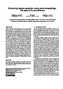
In Table 1 the number of generations are described needed to solve the task with the original NEAT method. Number of buckets Generations

5 1000 (ns)

15 1000(ns)

25 105

35 85

45 78

60 78

75 110

100 98

Table 1: NEAT: Number of Generations

The data from Table 1 is depicted in Figure 2. Using 5 or 15 number of buckets proved to be too low of a resolution of the data to solve the task. Using a numbers of buckets over 100 proved impossible due to overloading of the memory of the computers used. Although the data is rather fuzzy, the graph does show that using a moderate resolution of around 40 to 60 number of buckets gives the best performance using a minimal amount of generations to evolve a network that solves the task. Due to the nature of evolutionary methods, more experiments could be run to expose a more fixed solid line minimizing data anomalies. Besides the number of generations, another interesting aspect is the speed of evolution. This is an important aspect because it reveals how quickly the learning methods reaches the solving of the task condition. Additionally, it reveals which structural mutations are most influential on the fitness. Each generation champion has a certain fitness value. If these values are plotted until the task is solved a learning curve appears that shows when networks improve.

8

Automatic Feature Selection using FS-NEAT

Figure 2: NEAT: Number of Generations

Rather then depicting a table, a graph is plotted illustrating the learning curve of the various number of buckets in Figure 3.

Figure 3: NEAT Evolution of fitness Graph

Currently, no significant structural mutations have been identified. However, there might be an opportunity here for future work. 6.1.2

Evolved topology

The minimal required topology to solve the task added only a single hidden node with links to the inputs and output.

Section 6

Results

9

Table 2 below describes the number of links added to the hidden node for each number of buckets. Number of buckets Number of links

25 22

35 22

45 15

60 25

75 38

100 28

Table 2: NEAT: Number of links added to the hidden node

The data reveals that using a resolution of approximately 45 buckets returns a minimal amount of connections from the input to the hidden node. It should be noted that, contrary to FSNEAT, regular NEAT has connections between all input nodes and the output node. The data above describes the added links from the input to the hidden node. The hidden node has one link to the output node.

6.2

FS-NEAT Original Parameters Results

Below the results of the FS-NEAT method with the original parameters are described. 6.2.1

Number of generations

In Table 3 the number of generations are described needed to solve the task. Number of buckets Generations

25 341

30 223

45 305

60 289

75 196

100 NA

Table 3: FS-NEAT Original Parameters: Generations to solve task

The data from table 3 is depicted in Figure 4.

Figure 4: FS-NEAT Original Parameters: Number of Generations

Figure 4 does not explicitly show an optimal setting, however, it can be noticed that slightly higher number of buckets, around 75, perform better suggesting that the current data might contain anamolies.

10

6.2.2

Automatic Feature Selection using FS-NEAT

Evolved topology

Here the evolved topology of the networks will be examined. The experiments indicated that the minimal required topology to solve the task added only a single hidden node. Table 4 below describes the number of links added to the hidden node for each number of buckets. Number of buckets Number of links per hidden node

25 34, 6, 36, 7

35 14, 13

45 57

60 64

75 30, 15

Table 4: FS-NEAT Original Parameters: Links added to hidden node (25 buckets generated 4

hidden nodes) The data generated shows an interesting phenomenon. Rather then adding a single hidden node, the FS-NEAT method occasionally adds extra hidden nodes. The links described in Table 4 are links between the inputs and the hidden node. In Table 5 are the number of links created between the input nodes and the output node. Number of buckets Number of links to output

25 32

35 51

45 54

60 95

75 122

Table 5: FS-NEAT Original Parameters: Links added to output node

These numbers however are a bit skewed since more number of buckets also allow for more connections. (Note that 2 state variables are bucketized). The values are transformed into relative values in Table 6. Number of buckets Average connections per bucket

25 0.64

35 0.73

45 0.60

60 0.80

75 0.81

Table 6: FS-NEAT Original Parameters: Relative amount of connections expressed in average

connections per bucket Table 6 shows that 45 number of buckets has a minimal set of generated connections. Table 7 depicts the absolute amount of input nodes with no active link (= no connection). This table indicates how much inputs are not used by FS-NEAT to solve the task. Necessarily, these figures need to be adjusted to relative values, see Table 8. Number of buckets Number of inactive links

25 12

35 15

45 10

60 19

75 21

Table 7: FS-NEAT Original Parameters: Number of inactive links

Figure 5 illustrates the evolution speed. This is an important aspect because it reveals how quickly the learning methods reaches the solving of the task condition. Each generation champion has a certain fitness value. If these values are plotted until the task is solved a learning curve appears that shows when networks improve. Rather then depicting a table, a graph is plotted illustrating the learning curve of the various

Section 6

Results

11

Number of buckets Average connections per bucket

25 0.24

35 0.43

45 0.11

60 0.16

75 0.14

Table 8: FS-NEAT Original Parameters: Number of relative inactive links expressed in average

connections per bucket

Figure 5: FS-NEAT Original Paramters: Evolution of fitness graph

number of buckets in Figure 5. The graph shows a similar curve as with regular NEAT although the FS-NEAT method appears to need more generations to evolve a network that solves the task. This is not surprising because the FS-NEAT method starts with a far more simple topology then it’s original NEAT counterpart.

6.3

FS-NEAT Modified Parameters Results

Here the results are described from the FS-NEAT method with modified parameters. 6.3.1

Number of generations

In Table 9 the number of generations are described needed to solve the task with the FS-NEAT method with the modified parameter settings. Number of buckets Number of generations

25 71

35 132

45 243

60 143

75 239

100 NA

Table 9: FS-NEAT Modified Parameters: Number of Generations

The data from Table 9 is depicted in Figure 6. The data shows that the modified parameters of FS-NEAT find a solution quicker than NEAT with 25 number of buckets. This is a very interesting finding because it suggests that the ’head

12

Automatic Feature Selection using FS-NEAT

Figure 6: FS-NEAT Modified Parameters: Number of Generations

start’ NEAT has with the starting topology might backfire. There could be successfull policies for FS-NEAT to find with a simpler starting topology. 6.3.2

Evolved topology

Table 10 below describes the number of links added to the hidden node for each number of buckets. Number of buckets Number of links per hidden node

25 24, 9

35 13,34

45 23, 25, 17

60 32,21

75 30,13,30

Table 10: FS-NEAT Modified Parameters: Number of links to hidden node (multiple nodes

possible) In Table 11 are the number of links created between the input nodes and the output node. Number of buckets Number of links to output

25 27

35 34

45 45

60 98

75 81

Table 11: FS-NEAT Modified Parameters: Number of links to output node

Table 12 depicts the relative amount of connections for the inputs with the output. Number of buckets Average connections per bucket

25 0.54

35 0.49

45 0.50

60 0.83

75 0.54

Table 12: FS-NEAT Modified Parameters: Relative connections to output expressed in average

connections per bucket Table 13 depicts the absolute amount of input nodes with no active link (= no connection). This table indicates how much inputs are not used by FS-NEAT to solve the task. Necessarily, these figures need to be adjusted to relative values, see table 14.

Section 7

Conclusions

13

Number of buckets Number of inactive links

25 14

35 20

45 21

60 11

75 54

Table 13: FS-NEAT Modified Parameters: Absolute inactive links

Number of buckets Average connections per bucket

25 0.28

35 0.29

45 0.23

60 0.9

75 0.36

Table 14: FS-NEAT Modified Parameters: Relative inactive links expressed in average connec-

tions per bucket

Figure 7 depicts the learning curve of the FS-NEAT method with modified parameters.

Figure 7: FS-NEAT Modified Parameters: Evolution of fitness graph

Figure 7 illustrates a similar learning curve as the previous methods except for 25 buckets at which the FS-NEAT method with modified parameters seems to miss the solution.

7

Conclusions

So, what exactly does the generated data tells us? How do both methods differ from each other? Although not all the data is crystal clear, certain differences can be pointed out. These matters will be discussed in the following section. 7.0.3

Number of Generations performance

When comparing both methods on the number of generations needed to solve the task, regular NEAT clearly is a faster method. It takes regular NEAT fewer generations to evolve a network that solves the task. FS-NEAT also successfully evolves a network that can solve the tasks but

14

Automatic Feature Selection using FS-NEAT

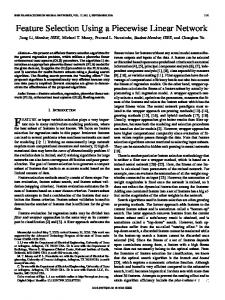
needs more generations. What we expected to find were results were the performance of NEAT could be described in the form of a normal curve. On low number of buckets NEAT would perform good because of the low complexity. The performance would increase until some optimal number of buckets. After that optimum, we expected performance to decrease because of increasing complexity. We would then expect FS-NEAT to outperform NEAT. The current experiments have illustrated the first part of that curve. Unfortunately, during these experiments we were unable to illustrate that second part of the curve with the results. Future work should focus on running experimentation to confirm or disconfirm our hypotheses about that second part of the curve. Figure 8 illustrates the compared performance differences between the various methods.

Figure 8: Comparison Graph: Number of generations

The graph shows what one should expect, a similar curvature between all methods but at varying heights. Obviously, NEAT solves the task in fewer generations because of its structural head start which is nicely illustrated in the graph. Strikingly, the FS-NEAT method with modified parameters seems to find the solution even quicker then NEAT. However, due to the use of genetic algorithms and the rather easy topology it is unclear whether it was a ’lucky shot’ or that FS-NEAT seriously outperforms NEAT on generation speed. Both methods show a similar fitness development curve in the evolved networks. However, when compared to each other, regular NEAT shows a steeper line in evolution. This, again, does not come as a surprise because regular NEAT starts out with connections between all the inputs and the output. These connections help the NEAT algorithm guide to a successful policy. The missing links of the FS-NEAT method do not provide such a guide, but allow for a topology that requires a minimal set of inputs. The data also suggests that, because of this implicit ’guide’ NEAT has with its starting topology, perhaps there are solution policies NEAT might miss that FS-NEAT might not. The FS-NEAT method with modified parameters found a successfull policy before NEAT. If this is a serious piece of data, rather than coincidence, then perhaps FS-NEAT might find ’closer’ succesful policies then NEAT in which case NEAT is hindered by

Section 8

Future work

15

its implicit guide. 7.0.4

Topology performance

When comparing topologies it is important to distinguish between a simple topology with a minimum amount of nodes and links and a topology that uses a minimal set of inputs. The data shows that FS-NEAT does not necessarily provide a more simple network because it occasionally generates more than one hidden node. Since only one hidden node is required to solve the task any extra added hidden node can be considered redundant. In that respect the NEAT method constantly delivers the most simplest network. However, one important feature of FS-NEAT is that it selects only the most relevant inputs. And it is here that FS-NEAT shines. The data shows that, in optimal performance, FS-NEAT generates links with 39% of the provided inputs inactive. This is important because this feature of FS-NEAT can be used to determine the most essential inputs of a given task. It is up to the task at hand to determine which kind of topology is required. Clearly, in this case a topology with a minimal amount of inputs is preferred to illustrate the input selection power of FS-NEAT. 7.0.5

Domain

The pole-balancing domain successfully shifts the focus of the learning to the inputs to illustrate the selective power of FS-NEAT. It also, however, allows for a simple topology to solve the task which, in combination with genetic algorithms, might return random data thus calling for results based on statistics. In the current settings, with long running time for experiments, this might not be the most suitable domain.

8

Future work

The experiments performed have not been the most efficient. Furthermore, the NEAT package used also has a series of features that did not always improve performance. These topics will be addressed in the following subsections.

8.1

Experiments

One of the largest bottlenecks in the data collection is the duration of the experiments. These experiments could last from a mere few minutes to a number of days. Obviously, gathering a large amount of data to back any conclusions is a serious time consuming task. For this reason, only a number of experiments have been performed. For future work it is suggested that the coding of the experiments should be optimized. This can be done by parallelizing the code so it can be run on multiple computers or, redesigning parts of the code so it can be run on a super computer (e.g. Sara). Other drawbacks in the experiments have been the NEAT package that was used. The original NEAT package used a series of measures to stimulate the evolution of networks by punishing stagnating networks. As can be seen in the data, this sometimes resulted in promising networks being punished (e.g. fitness reduced or deleted altogheter) prematurely. Experiments could thus take much longer than needed. Luckily this feature is removed in newer packages of NEAT and do not have to be dealt with manually. For future work it is advised to use the latest NEAT packge (e.g. rtNEAT).

16

8.2

REFERENCES

Method Improvements

The FS-NEAT method shows high potential in the current results. Data suggests there might be an opportunity for FS-NEAT to beat NEAT in the start of evolution by finding policies NEAT might miss because of its relative advanced starting topology. This needs to be confirmed by more accurate data but if this is true than FS-NEAT could be enhanced by ways of slimming down the starting topology even more. Perhaps a new method could be developed that combines NEAT and FS-NEAT. It starts off with different starting topologies and, intelligently, monitors the progress of both approaches. It could then decide to follow the most promising path of evolution. It is uncertain though, that a promising policy at the beginning of evolution might really be the best eventual solution. 8.2.1

Speed Improvements

Unfortunately, the policies developed could not be examined. There is room here for improvement because if certain structural mutations lead to a jump in fitness then this information could be used in evolution. For example, the hybrid method above could use this information to decide which path of evolution to prioritize.

8.3

Domain Improvements

In the current domain the input space consists mostly of relevant features because two state variables have been bucketized. Perhaps an approach in which the state space is enlarged with true (random) redundant features could more accurately illustrate the power of FS-NEAT.

References [1] K.O. Stanley and R. Miikkulainen. Evolving Neural Network through Augmenting Topologies. Evolutionary Computation, 10(2):99–127, 2002. [2] S. Whiteson, P. Stone, K.O. Stanley, R. Miikkulainen, and N. Kohl. Automatic feature selection in neuroevolution. Proceedings of the 2005 conference on Genetic and evolutionary computation, pages 1225–1232, 2005.

IAS reports This report is in the series of IAS technical reports. The series editor is Bas Terwijn ([email protected]). Within this series the following titles appeared: not yet kown not yet kown Technical Report IAS-UVA-08-01, Informatics Institute, University of Amsterdam, The Netherlands, April 2008. F.A. Oliehoek and N. Vlassis and M.T.J. Spaan, Properties of the QBG-value function Technical Report IAS-UVA-07-04, Informatics Institute, University of Amsterdam, The Netherlands, August 2007. G. Pavlin and P. de Oude and M.G. Maris and J.R.J. Nunnink and T. Hood A Distributed Approach to Information Fusion Systems Based on Causal Probabilistic Models. Technical Report IAS-UVA-07-03, Informatics Institute, University of Amsterdam, The Netherlands, July 2007. All IAS technical reports are available for download at the ISLA website, http: //www.science.uva.nl/research/isla/MetisReports.php.