Author’s Accepted Manuscript Automatic Feature Learning Using Multichannel ROI Based on Deep Structured Algorithms for Computerized Lung Cancer Diagnosis Wenqing Sun, Bin Zheng, Wei Qian www.elsevier.com/locate/cbm
PII: DOI: Reference:
S0010-4825(17)30092-6 http://dx.doi.org/10.1016/j.compbiomed.2017.04.006 CBM2642
To appear in: Computers in Biology and Medicine Received date: 22 January 2017 Revised date: 10 March 2017 Accepted date: 11 April 2017 Cite this article as: Wenqing Sun, Bin Zheng and Wei Qian, Automatic Feature Learning Using Multichannel ROI Based on Deep Structured Algorithms for Computerized Lung Cancer Diagnosis, Computers in Biology and Medicine, http://dx.doi.org/10.1016/j.compbiomed.2017.04.006 This is a PDF file of an unedited manuscript that has been accepted for publication. As a service to our customers we are providing this early version of the manuscript. The manuscript will undergo copyediting, typesetting, and review of the resulting galley proof before it is published in its final citable form. Please note that during the production process errors may be discovered which could affect the content, and all legal disclaimers that apply to the journal pertain.
Automatic Feature Learning Using Multichannel ROI Based on Deep Structured Algorithms for Computerized Lung Cancer Diagnosis Wenqing Sun1, Bin Zheng2, Wei Qian1*
1
College of Engineering, University of Texas at El Paso, El Paso, Texas, United States
2
College of Engineering, University of Oklahoma, Norman, Oklahoma, United States
[email protected] http://ee.utep.edu/facultyqian.htm *
Corresponding author. Professor Department of Electrical and Computer Engineering, Director: Medical Imaging Informatics Laboratory, College of Engineering, University of Texas, El Paso, 500 West University Avenue, El Paso, Texas 79968, PH: (915) 747-8090, FX: (915) 747-7871
Abstract This study aimed to analyze the ability of extracting automatically generated features using deep structured algorithms in lung nodule CT image diagnosis, and compare its performance with traditional computer aided diagnosis (CADx) systems using hand-crafted features. All of the 1018 cases were acquired from Lung Image Database Consortium (LIDC) public lung cancer database. The nodules were segmented according to four radiologists’ markings, and 134668 samples were generated by rotating every slice of nodule images. Three multichannel ROI based deep structured algorithms were designed and implemented in this study: convolutional neural network (CNN), deep belief network (DBN), and stacked denoising autoencoder (SDAE). For the comparison purpose, we also implemented a CADx system using hand-crafted features including density features, texture features and morphological features. The performance of every scheme was evaluated by using a 10-fold cross-validation method and an assessment index of the area under the receiver operating characteristic curve (AUC). The observed highest area under the curve (AUC) was 0.899±0.018 achieved by CNN, which was significantly higher than traditional CADx with the AUC= 0.848±0.026. The results from DBN was also slightly higher than CADx, while SDAE was slightly lower. By visualizing the automatic generated features, we found some meaningful detectors like curvy stroke detectors from deep structured schemes. The study results showed the deep structured algorithms with automatically generated features can achieve desirable performance in lung nodule diagnosis. With well-tuned parameters and large enough dataset, the deep learning algorithms can have better performance than current popular CADx. We believe the deep learning algorithms with similar data preprocessing procedure can be used in other medical image analysis areas as well. Index Terms— Big data, deep learning, lung cancer, unsupervised feature learning, computer aided diagnosis
I. INTRODUCTION nspired by the human brain’s architecture, deep learning algorithms have been attracting more and more researchers’ attentions in the past ten years [1]. Compared to traditional machine learning algorithms with shallow architectures, the deep learning algorithms are organized in a deep structure with several levels of composition of non-linear operations in the learned functions. Like the deep architecture of the brain, a given input percept represented at multiple levels of abstraction in the algorithm, and each level corresponds to a different area of cortex [2]. This architecture allows the algorithm to automatically learn features at multiple levels of abstraction so that it can generate the complex functions linking the input to the categories directly from raw data without using human-crafted features (i.e. manually designed features). The features extracted higher level of the hierarchies is composed by the weighted combination of the features of lower levels, and each level contains hundreds or thousands of neurons. In computer vision areas, feature design is the most challenging and time consuming part, and the ability to automatically extract features from raw data is extremely attractive especially in the age of big data.
I
The primary task for big data analytics is discriminative analysis. In recent years with the development of cloud storage and the explosion of big data, the sizes of available digital image collections have been increasing rapidly. These images were generated from a variety of sources such as social networks, cloud services, global positioning satellites, clinical imaging systems, military surveillance, and security systems [3]. To efficiently classify these massive images, automatically extracting semantic information from these images with deep structured algorithms is the most popular and promising method. Their advantages in constructing high level complicated representations from multiple domains of the original image captured the attention from big companies like Facebook, Google, IBM to invest millions of dollars every year in deep learning research, and recently has begun topping the companies benefit [3][4]. Learning from the deep, layered and hierarchical models of data, numerous study results showed that deep learning algorithms can outperform the traditional machine learning models in many different tasks, including speech recognition [5][6][7], computer vision [1][5] [6], and natural language processing [7][8][9]. Compared to its early stage, deep learning applications have already extended from simple image classifications, like handwritten numbers recognition, to more complicated classification tasks. In ImageNet LSVRC-2012 contest, the winner group successfully designed the deep learning algorithm and classified 1.2 million high-resolution images into 1000 different categories at the error rate of 15.3%, compared to 26.2% reported by the second-best group who didn’t use deep learning algorithms [6]. Dean et al. [10] used large-scale software infrastructure based deep learning models made further success on a visual object recognition task with 16 million images and 21k categories. In another contest, deep learning algorithms beat other algorithms and won MICCAI 2013 grand challenge and ICPR 2012 mitosis detection Contest [11]. In 2015, Shen et al. [12] diagnosed lung cancer on LIDC database using a multi-scale two layer convolutional neural network, and the reported accuracy was 86.84%. Kumar et al. [13] tested their algorithm using deep features extracted from autoencoder on 157 cases from the same dataset, and reached the accuracy of 75.01%. Healthcare industry is also facing the opportunities and challenges of big data. Reports said that at this rate of growth, healthcare data in United States will soon reach the zettabyte (10 12 gigabytes) scale [14]. If these big data can be effectively synthesized and analyzed, those relations, patterns and trends can be revealed, thus the doctors can provide more thorough and insightful diagnoses and treatments, and potentially resulting in higher quality care at lower costs [15]. With the development of precision medicine and radiomics, massive radiomics data collected from multiple modalities in a mineable form are gradually becoming available to build descriptive and predictive models [16]. Deep structured algorithms have the potential to generate valuable features and reveal the quantitative predictive or prognostic associations between raw data and medical outcomes. In the last three decades, many researchers have been developing computer aided diagnosis (CADx) algorithms or systems optimized to enhance the performance of radiologists reading and interpreting medical images [17][18][19]. Most of the previous researches were based on manually designed computational features, and these extracted features were sent to linear classifiers to distinguish the benign cases and malignant cases. These features include texture features, density features, morphological features extracted from the whole original image or region of interest (ROI). For example, area, circularity, ratio of semi-axis are typical and useful morphological features [20]; average intensity, mean gradient of region boundary, density uniformity are common density features used for mass detection [21]; wavelet features, gray-level co-occurrence matrix (GLCM) features, run length features, local binary pattern (LBP) features, SIFT features are useful texture features we used for breast cancer risk analysis [22]. Feature design is considered as an essential module for most existing CADx systems, but it is a time consuming and complicated task [13][23][24][25]. Moreover, the combination of well-designed features may not necessarily produce expected performance without considering the correlation and interaction among other features. Feature selection algorithms like genetic algorithm (GA), sequential forward floating selection (SFFS) can help generate the optimum feature combinations [26][27], but they become less efficient on high dimension features [28][29]. In addition, the performance and reproducibility of CADx systems are always controversial topics even for the commercially available systems [30][31]. Because different image databases were used to develop different schemes and the results depend heavily on the difficulty of the selected cases [32], and current CADx schemes are sensitive to small variations in the digital value matrices that result from operators and machines [33][34][35]. Some research groups already made some progress in using deep learning algorithms on lung cancer diagnosis: Wei Shen et al [36] proposed multiscale convolutional neural network structure on lung cancer diagnosis using 3D data, and they integrated information of ROIs acquired at different scales; Kumar Devinder et al [13] used autoencoder to analyze the diagnostic data from LIDC database. In this study, we tested the feasibility of using features automatically learned from deep structured algorithms using a large scale lung cancer computed tomography (CT) examinations for the early diagnosis of lung cancer. A multichannel ROI based deep learning scheme was developed, and three deep structured algorithms were designed and implemented in this study: Convolutional Neural Network (CNN), Deep Belief Networks (DBNs), and Stacked Denoising Autoencoder (SDAE). We compared the performance of our proposed deep learning scheme and current popular CADx scheme (i.e. traditional CADx system) with traditional hand-crafted features and also other deep learning techniques like transfer learning in nodules diagnosis. The details of methodologies and results are discussed in the following sections.
II. METHOD A. Dataset All the data we used in this study is from Lung Image Database Consortium and Image Database Resource Initiative (LIDC/IDRI) public database, which consists of diagnostic and lung cancer screening thoracic CT scans with marked-up annotated lesions [37][38]. At the time point of this study, there are 1018 cases collected from seven academic centers and eight medical imaging companies in this database with the CT scans slice thickness varies from 1.25 mm to 3 mm and reconstruction interval are between 0.625 mm and 3 mm. The clinical thoracic CT scan images of each case are associated to an XML file with the record of two-phase image annotation process evaluated by four experienced thoracic radiologists. Each radiologist reviewed each CT scan independently and labeled the lesions to one of the three categories: nodule larger than 3 mm, nodule less than 3 mm, and non-nodule larger than 3 mm. The final diagnosis were made in the unblinded-read phase based on four anonymized marks. As reported by [39], the mean pairwise kappa values of the blinded and unblinded reading phases were 0.25 and 0.39. The ratings of 5 malignancy levels were given from each of the four radiologists to all the nodules larger than 3 mm: level 1 and 2 represent benign nodules and level 4 and 5 denote malignant nodules. Fig. 1 shows an example of a nodule in original CT scan images and its boundaries marked by four radiologists. From these 1018 cases, we eliminated the cases with no larger than 3 mm nodules or non-nodule lesions only, incomplete cases, and cases with missing truth files. To avoid the partial volume effects caused by different CT scanning protocols across different vendors, bi-cubic interpolation was used to normalize CT scan volumes resulting in isotropic resolution at all directions. Since the size and shape of segmented nodules in the top layer and bottom layer might dramatically different from the rest of the slices, we removed these two slices if the segmented nodule volume contains three or more slices before interpolation. Then the segmented nodule area in each slice was set into a 52 by 52 pixel rectangular according to the following rules: if the segmented area can be fitted into a 52 by 52 pixel rectangular, it would be placed to the center of this rectangular; otherwise it would be downsampled to the size of 52 by 52. Every ROI was rotated to four different directions (0, 90, 180, 270), and converted to four single vectors with each representing one orientation. All the values in the vectors were downsampled to 8 bits. From these 1018 cases, 134668 samples were obtained and each sample has 2704 pixels. The distribution of malignancy levels of the data is shown in Table 1. All the intermediate samples (level 3) were eliminated, and 41372 benign samples (level 1 and 2) and 47576 malignant samples (level 4 and 5) were used for this study. Table 1: The distribution of malignancy levels of our dataset
Malignacy level
1
2
3
4
5
Total
Amount
15448
25924
45720
20520
27056
134668
Fig. 1: A nodule example in one slice of the original CT scan images with nodule’s boundary marked by four radiologists (left) and the zoomed in image (right)
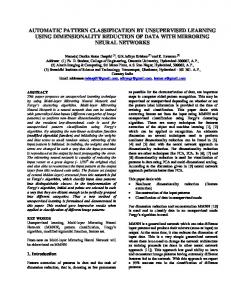
B. Method In this study, we designed and implemented a novel three channel image generating method and three state-of-the-art deep structured schemes for nodule diagnosis: CNN, DBN, and SDAE. And for the comparison reason, we also extracted hand-crafted features from three different feature categories to classify the nodules. In this section, we will introduce every scheme used in this study respectively. (1) Three channel image generation: For each segmented gray level ROI patches, we generated three images: original ROI including nodules and surrounding areas, nodule only image and gradient image. The nodule image highlighted the shape information of the nodule, and the gradient image is focused on the texture of the image. Then all the three images were combined as a RGB channel to generate the
three channel RGB images. Figure 2 shows an example of three channel ROI and its three corresponding channels.
Figure 2: An example of three channel ROI: (a) original ROI, (b) nodule ROI, (c) gradient ROI, (d) the three channel ROI.
(2) Convolutional Neural Network: Convolutional neural network is the only deep learning algorithm we used without the need of unsupervised pre-training. Because the neural network with several full-connected layers is not practical for training when initialized randomly, the CNN structure we developed in this study is based on LeCun’s model: several convolutional layers and subsampling layers followed by a fully-connected layer, and every layer has a topographic structure [40][41]. The algorithm begins with extracting random sub-patches from the ROIs mentioned above, with the size of the sub-patches referred to as the “receptive field size”. In each layer the neuron is associated with a fixed two-dimensional position and its receptive field is corresponding to the input from previous layer (the first layer is corresponding to the original input image). Several neurons are connected to the same location at every layer, and each neuron is a linear combination of its corresponding neurons in previous layer with its set of input weights. The neurons at different locations are associated with the same set of weights, but different corresponding input patches [2]. The architecture of the proposed CNN is summarized in Fig. 2. It contains 9 layers: the first and last layer are input layer and output layer, and the 2, 4, 6 layers are convolutional layers, and the 3, 5, 7 layers are subsampling layers, and the last layer is the fully connected layer. In particular, the second layer has 12 feature maps connected to the input image through 12 5 5 kernels, followed by a 2 2 average pooling layer. The fourth layer has 8 feature maps, and they are all connected to the previous layers through 96 5 5 kernels. After another average pooling layer, we obtained the sixth layer with 6 feature maps, and 48 5 5 kernels were used for this layer. In the eighth layer, the input was shrunk to 3 3 matrices, and they were fully connected by using softmax non-linearity to the 2 output neurons associating with benign and malignant nodules. The output of each layer was contrast normalized and whitened before sending to the next layer [42]. The batch size was set to 100 and the learning rate was set to 0.1 for 100 epochs, the subsampling rate was constantly 2.
Fig. 2: The structure of CNN designed in this study. It demonstrates the original image, all the feature maps in convolutional layer, the process of subsampling layer. Wi is the weight matrix in each kernel, X i is the pixels values of in a patch, and hki,j is one hidden unit in layer k at location (i, j).
(3) Deep Belief Networks Another deep learning algorithm we designed and tested in this study was DBN, it is a generative model that combined directed and undirected connections between variables. The model was obtained by training and stacking four layers of
Restricted Boltzmann Machine (RBM) in a greedy fashion. The RBM was used for the unsupervised learning as the start of the algorithm, and the meaningful computational features can be automatically extracted from the training process. The distribution of visible layer x can be calculated by computing the energy function of RBM: ( ) , where h is the vector of hidden units, b and c are the bias vectors and W is the weight connecting two adjacent layers. Each of the first three layers of our proposed scheme contains 400 units, and the top layer contains 1600 units. RBM doesn’t allow the interactions either between the hidden units or between visible units with each other. The DBN we designed in this study followed the work of Hinton et al. [1], training greedily from lowest layer to the highest layer as an RBM, and the activations of previous layers were served as the input of next layer. The distribution of hidden unit hj in the layer i follows the formula: (
()
|
(
)
|
( )
)
(
()
(
)
(
)
);
the distribution visible unit xj follows: (
)
(
( )
( )
( )
).
When we reshape each weight vector into an image patch, each value was associated to the pixels at the same position of the input ROI. The positive and negative values of the pixel values at each position represent the possibility increase or decrease of being 1 of the hidden units. This weight can be treated as the features extracted from the original ROI automatically by the computer. Once a layer is trained, all the parameters including the automatically learnt features were fixed until the whole training procedure for the multilayer DBN was finished. This greedy algorithm was shown to be optimizing the variational lower-bound on the data likelihood, if units in higher layers at least as have many units as each of the lower layers [43]. For multichannel ROIs, each channel was transferred into a vector and the input was formed by connecting these three vectors together. The batch size was also set to 100, and the learning rate was set for 0.01 for 100 epochs. The neural network was connected for the supervised learning. The brief idea of the DBN architecture used in this study is shown in Fig. 3.
Fig. 3: The structure of DBN designed in this study. h(i) is the vector of hidden units in hidden layer i, and W(i) is the weight connecting two layers
(4) Stacked Denoising Autoencoder The last deep learning model we implemented and tested was SDAE [5] and each autoencoder was stacked on the top of each other with the structure very similar to the DBN mentioned above. Autoencoder is another unsupervised algorithm that can automatically extract features from the data, and it is a type of feed forward neural network trained to reproduce the original input at the output layer instead of classifying them into different classes. The autoencoder consists encoder module and decoder module, and the encoder of layer i can be expressed as: () ( ) ( () ) () { ( ) ( ) ( ̃) and the decoder of layer i can be expressed as:
{
()
( ̂
(
()
(
( )
)
(
)
)
( )
(
)
)
where ̃ is the original input vector with randomly added noise and ̂ is the output vector, h is the vector of hidden units, W is the weight between adjacent layers, b and c are the bias vectors, sigm means the sigmoid function [44]. All the parameters were optimized by minimizing the loss function below during the training process: ∑( ̂
)
where ̂ and are the element in the noiseless input vector and output vector, and len is the total element amount of the vector. For the discrimination purpose, the supervised classifier was added to the last layer of the encoder, and the whole model was trained as a feedforward-backpropagate neural network [45].
There were 2000, 1000, and 400 hidden neurons in each autoencoder with corruption level of 0.5. Fig. 4 shows the structure of the proposed SDAE. The size of batches was set to 100, and the learning rate was set to 1 for all the 100 epochs. After the unsupervised autoencoder being well-trained, all the parameters were frozen and the weights were used to initiate the supervised neural network for classification.
Fig. 4: The structure of designed SDAE. Wi is the weight matrix for layer i in encoder; WiT is the weight for decoder and it is the transpose of Wi.
(5) Traditional hand-crafted features For the comparison purpose, we extracted the traditional hand-crafted features from the same ROIs. From our previous experience of developing CADx systems, there are three major categories of computational features: morphological features, density features, and texture features. In this study, we implemented and tested several typical features in each category, and all these features were used in our previous researches and proved to be effective. 40 features were extracted from three categories and seven feature groups, and Table 2 listed the descriptions of all these features. Then a shallow artificial neural network (ANN) was used to train the classifier using features from the same categories. We also combined all the features together, and trained the ANN classifier again using the features selected by SFFS.
Table 2: Descriptions of the traditional hand-crafted features used in this study
Category
Feature descriptions
Morphological Density
1) Area, 2) circularity, 3) ratio of semi-axis 4) Average intensity, 5) standard deviation, 6) entropy GLCM
7) Mean, 8) variance, 9) correlation, 10) uniformity, 11) inertia, 12) inverse difference, 13) contrast, 14) sum entropy, 15) homogeneity, 16) angular second moment
Wavelet
17-20) Mean and 21-24) variance of HH, HL, LH, LL
Run length
25-26) Long run emphasis, 27-28) short run emphasis, 29-30) low gray-level run emphasis, 31-32) high gray-level run emphasis, 33-34) run percentage calculated at 0 and 90 degree
LBP
35) first and 36) second PCA component of LBP histogram
SIFT
37-40) first PCA components of four SIFT bin histogram
Texture
C. Experimental design and evaluation
To compare the performance of the deep learning features and traditional hand-crafted features, we tested all the algorithms based on the same ROIs extracted by the method mentioned above. Since some ROIs extracted from the same case, in order to completely separate the training data and testing data, we applied 10-fold cross-validation method based on cases rather than slices, and all the ROIs associated to the cases from the training folds were used for training, while the ROIs corresponding to the cases from the testing fold were used for testing. To evaluate the performance, we calculated the ROI based AUC and nodule based AUC. AlexNet based transfer learning were also used in this experiment for comparison, and it was trained on the last 1 to 3 layers. All the tests were two-sided and p value