Automatic Fence Insertion in Integer Programs via Predicate Abstraction

Automatic Fence Insertion in Integer Programs via Predicate Abstraction? Parosh Aziz Abdulla1 , Mohamed Faouzi Atig1 , Yu-Fang Chen2 , Carl Leonardsson1 , and Ahmed Rezine3 1

Uppsala University, Sweden Academia Sinica, Taiwan Link¨oping University, Sweden 2

3

Abstract. We propose an automatic fence insertion and verification framework for concurrent programs running under relaxed memory. Unlike previous approaches to this problem, which allow only variables of finite domain, we target programs with (unbounded) integer variables. The problem is difficult because it has two different sources of infiniteness: unbounded store buffers and unbounded integer variables. Our framework consists of three main components: (1) a finite abstraction technique for the store buffers, (2) a finite abstraction technique for the integer variables, and (3) a counterexample guided abstraction refinement loop of the model obtained from the combination of the two abstraction techniques. We have implemented a prototype based on the framework and run it successfully on all standard benchmarks together with several challenging examples that are beyond the applicability of existing methods.

1

Introduction

Modern concurrent process architectures allow relaxed memory, in which certain memory operations may overtake each other. The use of weak memory models makes reasoning about the behaviors of concurrent programs much more difficult and error-prone compared to the classical sequential consistency (SC) memory model. In fact, several algorithms that are designed for the synchronization of concurrent processes, such as mutual exclusion and producer-consumer protocols, are not correct when run on weak memories [3]. One way to eliminate the non-desired behaviors resulting from the use of weak memory models is to insert memory fence instructions in the program code. A fence instruction forbids certain reordering between instructions issued by the same process. For example, a fence may forbid an operation issued after the fence instruction to overtake an operation issued before it. Recently, several research efforts [9, 8, 14, 6, 15, 13, 18, 5, 4, 10, 11, 2] have targeted developing automatic verification and fence insertion algorithms of concurrent programs under relaxed memory. However, all these approaches target finite state programs. For the problem of analyzing algorithms/programs with mathematical integer variables (i.e., variables of an infinite data domain), these approaches can only approximate them by, e.g., restricting the upper and lower ?

This research was in part funded by the Uppsala Programming for Multicore Architectures Research Center (UPMARC).

bounds of variables. The main challenge of the problem is that it contains two different dimensions of infiniteness. First, under relaxed memory, memory operations may be temporarily stored in a buffer before they become effective and the size of the buffer is unbounded. Second, the variables are ranging over an infinite data domain. In this paper, we propose a framework (Fig. 1) that can automatically verify a concurrent system S (will be defined in Sec. 2) with integer variables under relaxed memory and insert fences as necessary to make it correct. The framework consists of three main components. The first component (Sec. 4) is responsible for finding a finite abstraction of the unbounded store buffers. In the paper, we choose to instantiate it with a technique introduced in [15]. Each store buffer in the system keeps only the first k operations and makes a finite over-approximation of the rest. For convenience, we call this technique k-abstraction in this paper. The second component (Sec. 5) (1) finds a finite abstraction of the data and then (2) combines it with the first abstraction to form a finite combined abstraction for both the buffer and data. For the data abstraction, in this paper we choose to instantiate it with predicate abstraction; a finite set of predicates over integer variables in the system is applied to partition the infinite data domain into finitely many parts. The combined abstraction gives us a finite state abstraction of the concurrent system S . A standard reachability algorithm (Sec. 6) is then performed on the finite abstraction. For the case that a counterexample is returned, the third component analyzes it (Sec. 7) and depending on the result of the analysis it may refine the concurrent system by adding fences, refine the abstract model by increasing k or adding more predicates, or report that ce is an unpreventable counterexample trace, i.e., a bad behavior exists even in the SC model and cannot be removed by adding fences.

Concurrent System S Reachability Checking Algorithm (Sec. 6)

Counter Example ce

Counter Example Analysis (Sec. 7) Case (1)

Safe

Bug in SC

Abstraction of Buffers (Sec. 4)

Case (2) Add new fences Case (3)

Abstraction of Variables (Sec. 5)

Increase k Case (4) Add new predicates

Case (1) ce is feasible under SC Case (2) ce is infeasible under SC, but feasible under TSO Case (3) ce is infeasible under TSO, but feasible under k-abstraction Case (4) ce is infeasible under k-abstraction, but feasible under comb-abstraction

Fig. 1. Our fence insertion/verification framework

Because of the space limit and in order to simplify presentation, we demonstrate our technique under the total store order (TSO) memory model. However, our technique can

be generalized to other memory models such as the partial store order (PSO) memory model. In this paper, we use the usual formal model of TSO, developed in, e.g., [20, 23], and assume that it gives a faithful description of the actual hardware on which we run our programs. Conceptually, the TSO model adds a FIFO buffer between each process and the main memory (Fig. 2). The buffer is used to store the write operations performed by the process. Thus, a process executing a write operation inserts it into its store buffer and immediately continues executing subsequent operations. Memory updates are then performed by non-deterministically choosing a process and executing the oldest write operation in its buffer. A read operation by a process p on a variable x can overtake some write operations stored in its own buffer if all these operations concern variables that are different from x. Thus, if the buffer contains some write operations to x, then the read value must correspond to the value of the most recent write operation to x. Otherwise, the value is fetched from the memory. A fence means that the buffer of the process must be flushed before the program can continue beyond the fence. Notice that the store buffers of the processes are unbounded since there is a priori no limit on the number of write operations that can be issued by a process before a memory update occurs. To our knowledge, our approach is the first automatic verification and fence insertion method for concurrent integer Read x, value of x is in the buffer. programs under relaxed memory. We implemented a prototype and run it successMemory (x, 5) (y, 7) (x, 4) (y, 3) ← Process p x=8 fully on all standard benchmarks together y=7 Read y, value of y is NOT in the buffer. with challenging examples that are be(x, 3) (x, 2) (x, 7) (x, 2) ← Process q yond the applicability of existing methods. For instance, we can verify Lamport’s Bakery algorithm without assumFig. 2. TSO memory model. ing an upper bound on ticket numbers.

2

Concurrent Systems

Our goal is to verify safety properties of concurrent systems under relaxed memory. A concurrent system (P, A, XS , XL ) consists of a set of processes P running in parallel with shared variables XS and local variables XL . These processes P are modeled by a set of finite automata A = {A p | p ∈ P}. Each process p in P corresponds to an automaton A p in A. Each local variable in XL belongs to one process in P, i.e., we assume that two processes will not use the same local variable in XL . The automaton A p is a triple (Q p , qinit p , δ p ), where Q p is a finite set of program locations (sometimes “locations” for short), qinit p is the initial program location, and δ p is a finite set of transitions. Each transition is a triple (l, op, l 0 ), where l, l 0 are locations and op is an operation in one of the following forms: (1) read operation read(x, v), (2) write operation write(x, v), (3) fence operation f ence, (4) atomic read write operation arw(x, v, w), (5) assignment operation v := e, and (6) guard operation e1 ◦ e2 , for ◦ ∈ {>, =, representing arbitrary integer values and assigning the initial values of all shared and local variables to >.

(M, L, pc, B) to a next configuration (M 0 , L0 , pc0 , B0 ) if the following hold: (1) pc(p) = l, pc0 (p) = l 0 , ∀q ∈ P.q 6= p → pc(q) = pc0 (q) and (2) at least one of the transition rules in Fig.3 is satisfied. Below we explain the rules in Fig.3. |B p | = i

¬Contain(x)

Contain(x) L’(v)=LastWrite(x)

READ-B

L’(v)=M(x) Empty M(x) = L(v)

READ-M

B0x (b p,i+1 ) = x B0v (b p,i+1 ) = L(v)

WRITE

ASSIGN e1 [L] ◦ e2 [L] ARW M 0 (x) = L(w) L0 (v) = e[L] FENCE GUARD |B p | = i Bx (b p,1 ) = x1 . . . Bx (b p,i ) = xi Bv (b p,1 ) = v1 . . . Bv (b p,i ) = vi

Empty

M 0 (x1 ) = v1 B0x (b p,1 ) = x2 . . . B0x (b p,i−1 ) = xi B0v (b p,1 ) = v2 . . . B0v (b p,i−1 ) = vi B0x (b p,i ) = B0v (b p,i ) = ⊥

UPDATE

Fig. 3. Transition Rules of a Transition System under TSO. The conditions above the horizontal line are the “pre-condition” that decide whether this transition can be triggered and those below the line are the “post-condition” that decide what the next configuration should be. For a more clear presentation, in the post-condition of the rules defined in this paper (including those in the other sections), we focus only on the component that has been changed. For the components that has not been changed, we assume implicitly that the primed version (the component in the next configuration) is equal to the non-primed version (the same component in the current configuration). For example, for all shared variables x ∈ XS , if M 0 (x) has not been assigned a value in the rule, we assume implicitly M 0 (x) = M(x).

READ-B rule: When op=read(x, v), if the buffer of p contains write operations to x, we read the value of the last write operation to x in p’s buffer. We use Contain(x) as a shorthand for (∃i ∈ N .Bx (b p,i ) = x), or, informally, there exists some write operations to x in the buffer. We use LastW rite(x) to denote the most recent value written to x in the buffer of p. Formally, LastW rite(x) = Xv (b p,i ), where i = Max({ j ∈ N | Bx (b p, j ) = x}). READ-M rule: When op=read(x, v), if the buffer of p does not contain write operations to x, we read the value of x from the memory. WRITE rule: When op=write(x, v), we put the operation (x, v) to the end of the buffer. We use |Bp | to denote the length of the buffer of p. Notice that this number equals the index of the most recent operation in p’s buffer. Formally, |Bp | = Max({j ∈ N | Bx (bp,j ) 6= ⊥} ∪ {0}). FENCE rule: When op=fence, the transition can be executed only when the buffer of p is empty. Here we use the predicate Empty as a shorthand for Bx (b p,1 ) = ⊥. ARW rule: When op=arw(x,v,w), the transition can be executed only when the buffer of p is empty and the value of x in the memory equals the value of v in p. When it is executed, the value of x in the memory is immediately changed to the value of w in p. UPDATE rule: The write operations in the buffer can be at any time nondeterministically delivered to the memory. This is handled by implicitly adding self-loop transitions update

update

l −−−−→ l from all the locations in Q. Notice that the transition l −−−−→ l is internal, i.e., it never appears explicitly in the definition of the concurrent system. In this rule, the oldest operation in p’s buffer (the one with index 1) will be used to update the memory while all the other operations in the buffer are shifted one step closer to the memory, i.e., their indices are reduced by 1.

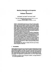
ASSIGN rule: When op = (v := e), where e is a Presburger expression over XL , we update the value of v to the evaluation of e under the assignment L (denoted as e[L]). GUARD rule: When op = (e1 ◦ e2 ), where e1 and e2 are Presburger expressions over XL , the transition can be executed only when (e1 [L] ◦ e2 [L]) holds, i.e., the evaluations of e1 and e2 under L is in the binary relation ◦. Here we let ◦ ∈ {>, =, y ∧ b p,4 = t ∧ lw p,y = t) while we store the control component exactly. We call the result a comb-abstract configuration. In the example, the comb-abstract configuration encodes k-abstract configurations with the same control components and with data components satisfying the constraint defined in the predicate f . Taking the k-abstract configuration (M, L, pc, Bx , Bv , S, R) 4 on the top-right of Fig 6 as an example, it has the 4

Recall that S : P → 2XS records, for each process in P, the set of variables in the TSO buffer with index larger than k, and R : XLW → Z is a partial function that records the most recent value of each shared variable in the buffer.

k-Abstract Configurations R(lw p,x ) = 1, R(lw p,y ) = 4

Comb-Abstract Configuration

x

y

y

y

x

y

x

x

x, y

←

p: pc = l3

←

q: pc = l4

encodes

(y, 4)

(y, 7)

(y, 4)

(x, 3)

(y, 2)

(x, 7)

(x, 2)

x=8 y=7 x, y

←

p: s=3 t =4 pc = l3

←

q: u=2 v=5 pc = l4

←

p: s=5 t =2 pc = l3

←

q: u=4 v=3 pc = l4

R(lwq,x ) = 2, R(lwq,y ) = 1

...

f =x > y ∧ b p,4 = t ∧ lw p,y = t

(x, 1)

R(lw p,x ) = 3, R(lw p,y ) = 2 (x, 3)

(y, 4)

(y, 5)

(y, 2)

(x, 5)

(y, 1)

(x, 3)

(x, 3)

x=4 y=3

R(lwq,x ) = 5, R(lwq,y ) = 5

x, y

Fig. 6. A comb-abstract configuration and the k-abstract configurations it encodes. Here XS = {x, y} and XL = {s,t, u, v}. All the configurations in the figure have the same control components pc, Bx , and S, where pc(p) = l3 ∧ pc(q) = l4 , Bx (b p,1 ) = Bx (bq,1 ) = Bx (bq,3 ) = Bx (bq,4 ) = x ∧ Bx (b p,2 ) = Bx (b p,3 ) = Bx (b p,4 ) = Bx (bq,2 ) = y, and S(p) = 0/ ∧ S(q) = {x, y}.

same control components as the comb-abstract configuration on the left. By substituting x and y in f with M(x) and M(y), t with L(t), b p,4 with Bv (b p,4 ), lw p,y with R(lw p,y ), we obtain the formula 8 > 7 ∧ 4 = 4 ∧ 4 = 4, which evaluates to true. Hence it is a k-abstract configuration encoded by the comb-abstract configuration.

5.3

Comb-Abstract Configurations

Formally, a comb-abstract configuration is a tuple ( f , pc, Bx , S), where f is a formula over X that encodes data components, and the control components pc, Bx , S are defined in a similar manner as in a k-abstract configuration. Given a k-abstract configuration ck = (M, L, pc, Bx , Bv , S, R) and a formula f over X, we define the evaluation of f in ck , denoted as f [ck ], as the value obtained by substituting all free occurrences of x ∈ XS in f with M(x), v ∈ XL in f with L(v), b ∈ XB in f with Bv (b), and lw ∈ XLW in f with R(lw). Given a comb-abstract configuration cc = ( f , pc, Bx , S), we define the concretization function γc (cc ) = {ck = (M, L, pc, Bx , Bv , S, R) | f [ck ]}. Given a set of combS abstract configurations Cb , we define γc (Cb ) = cb ∈Cb γc (cb ). Given a set of k-abstract configurations Ck , we use αc (Ck ) to denote the set of comb-abstract configurations that encodes exactly Ck , i.e., Ck = γc (αc (Ck )).

5.4

Predicate Abstraction

Let f be a formula over X and P a set of predicates over X. Each predicate in P partitions the valuation of variables in X into two parts. For each predicate π ∈ P such that f → π is valid, or equivalently, f ∧ ¬π is unsatisfiable, π characterizes a superset of data components of those characterized by f . The predicate abstraction function α pa ( f , P ) returns a conjunction of all predicates π ∈ P such that f → π is valid. 5.5

Comb-Abstract Transition Relation (w.r.t a Set of Predicates P ) op

Assume that we have l −→ p l 0 in the concurrent system S . There exists a comb-abstract transition w.r.t. P from the comb-abstract configuration ( f , pc, Bx , S) to a next configuration (α pa ( f 0 , P ), pc0 , B0x , S0 ) if the following hold (notice that we always apply predicate abstraction to the formula f 0 of the next configuration): (1) pc(p) = l, pc0 (p) = l 0 , ∀q ∈ P.q 6= p → pc(q) = pc0 (q), (2) f 0 is satisfiable, and (3) at least one of the combabstract transition rules in Fig.7 is satisfied. Contain(x) ¬Contain(x) READ-M READ-B f 0 = (∃X. f ∧ v0 = x ∧ Equ(X \ {v}))[x0 /x]x0 ∈X 0 f 0 = (∃X. f ∧ v0 = lw p,x ∧ Equ(X \ {v}))[x0 /x]x0 ∈X 0 |B p | = k ∨ S(p) 6= 0/ WRITE-G f 0 = (∃X. f ∧ lw0p,x = v ∧ Equ(X \ {lw0p,x }))[x0 /x]x0 ∈X 0 S0 (p) = S(p) ∪ {x} |B p | = i < k S(p) = 0/ WRITE-L Empty f 0 = (∃X. f ∧ b0p,i = lw0p,x = v ∧ Equ(X \ {b p,i , lw p,x }))[x0 /x]x0 ∈X 0 B0x (b p,i ) = x FENCE Empty ARW f 0 = (∃X. f ∧ x = v ∧ x0 = w ∧ Equ(X \ {x}))[x0 /x]x0 ∈X 0 |B p | = i 6= 0 Bx (b p,1 ) = x1 . . . Bx (b p,i ) = xi UPDATE-NE 0 0 B0x (b Vp,1 ) = x2 . . . Bx (b p,i−1 ) = xi Bx (b p,i ) = ⊥ f 0 = (∃X. f ∧ x10 = b p,1 ∧ 1≤k≤i−1 b0p,k = b p,k+1 ∧ Equ(X \ {x1 , b p,1 , . . . , b p,i−1 }))[x0 /x]x0 ∈X 0 x ∈ S(p) |B p | = 0 UPDATE-AM f 0 = (∃X. f ∧ Equ(X \ {x}))[x0 /x]x0 ∈X 0 x ∈ S(p) |B p | = 0 UPDATE-AS f 0 = (∃X. f ∧ x0 = lw p,x ∧ Equ(X \ {x}))[x0 /x]x0 ∈X 0 S0 (p) = S(p) \ {x} ASSIGN f ∧ (e1 ◦ e2 )} f 0 = (∃X. f ∧ v0 = e ∧ Equ(X \ {v}))[x0 /x]x0 ∈X 0 GUARD

Fig. 7. Comb-Abstract Transition Rules. We use the predicate Equ(V ) to denote v∈V v0 = v, i.e., no change made to variables in V in this transition. We assume all bounded variables are renamed to fresh variables that are not in X ∪ X 0 so the substitution will not assign the names of bounded variables to some free variable. V

6

The Reachability Checking Algorithm

Alg.1 solves they reachability problem of a comb-abstract system derived from a given concurrent system. The inputs of the algorithm include a value k, a set of predicates P , a concurrent system S = (P, A, XS , XL ), and a partial function Bad : P → Q. We

Algorithm 1: Reachability Algorithm 1 2 3 4 5 6 7 8 9 10 11 12

Input : S = (P, A, XS , XL ), an integer k, a set of predicates P , a partial function Bad : P → Q Output: Either the program is safe or a counterexample ce / ∧ ∀b ∈ XB .Bx (b) = ⊥; cinit = (true, pc, Bx , S), where ∀p ∈ P.(pc(p) = qinit p ∧ S(p) = 0) / Next:={(cinit , ε)}, Visited:=0; while Next 6= 0/ do Pick and remove ((pd, pc, Bx , S), ce) from Next; if ∀p ∈ P.Bad(p) 6= ⊥ → pc(p) = Bad(p) then return ce is a counterexample; if ∃( f , pc, Bx , S)∈Visited then replace it with ( f ∨pd, pc, Bx , S) else add (pd, pc, Bx , S) to Visited; op

foreach l −→ p l 0 such that pc(p) = l do foreach comb-abstract transition rule r do op compute the next configuration (pd 0 , pc0 , B0x , S0 ) of (pd, pc, Bx , S) w.r.t l −→ p l 0 , r, and P ; if ¬(∃( f , pc0 , B0x , S0 )∈Visited s.t. pd 0 → f ) then op add ((pd 0 , pc0 , B0x , S0 ), ce · (l −→ p l 0 , r)) to Next; return The program is safe;

first generate the initial comb-abstract configuration cinit = (true, pc, Bx , S), where ∀p ∈ / ∧ ∀b ∈ XB .Bx (b) = ⊥. P.(pc(p) = qinit p ∧ S(p) = 0) For the reachability algorithm, we maintain two sets, Next and Visited (Line 2). Next contains pairs of a comb-abstract configuration c and a path that leads to c. Visited contains comb-abstract configurations that have been visited. Notice that Visited stores comb-abstract configurations in an efficient way; if both the comb-abstract configurations ( f1 , pc, Bx , S) and ( f2 , pc, Bx , S) should be put into Visited, we put ( f1 ∨ f2 , pc, Bx , S) instead. When Next is not empty (Line 3), a pair ((pd, pc, Bx , S), ce) is removed from Next and the algorithm tests if (pd, pc, Bx , S) encodes some bad TSO configurations (Line 5). For the case that it does, the algorithm stops and returns ce as a counterexample. Otherwise (pd, pc, Bx , S) is merged into Visited (Line 6). Then the reachability algorithm explores the next configurations of (pd, pc, Bx , S) w.r.t the transitions in S and the comb-abstract transition rules (Lines 7-11). Once Next becomes empty, the algorithm reports that the program is safe. Notice that in the counterexample ce, we record not only the sequence of transitions of S but also the sequence of transition rules that have been applied. We need this in order to remove non-determinism in the comb-abstract system and thus simplify the counterexample analysis. To be more op specific, assume that l −→ p l 0 and a comb-abstract configuration c is given, it is possible that there exists more than one transition rules that can be applied and thus the same op transition l −→ p l 0 may lead to two different comb-abstract configurations. For example, assume that op = update and the length of the TSO buffer is larger than k. It could happen that both of the rules UPDATE-AM and UPDATE-AS can be applied. Then the current comb-abstract configuration c may have two different next comb-abstract op configurations w.r.t the same transition l −→ p l 0 .

7

Counter Example Guided Abstraction Refinement

The counterexample detected by the reachability checking algorithm is a sequence of pairs in the form of (δ, r), where δ is a transition in S and r is a comb-abstract transition op1 op2 opn 0 rule. Let ce = (l1 −−→ −→ p2 l20 , r2 ) . . . (ln −−→ pn ln0 , rn ) be the counterexample p1 l1 , r1 )(l2 −

returned from the reachability module. We next analyze ce and decide how to respond to it. Four possible responses are described in Fig.1. Case (1): We will not formally define the transition system induced from the concurrent system under sequential consistency (SC) model for lack of space. Informally, under the SC model, all operations will be immediately sent to the memory without buffering. We simulate ce under SC and if ce is feasible under SC, ce is not a bug caused by the relaxation of the memory model. In this case, it cannot be fixed by just adding fences. The algorithm reports that ce is a bug of the concurrent system under the SC model. Case (2): We can check if the counterexample ce is feasible under TSO by simulating it on the TSO system following the rules defined in Fig. 3. For the case that ce is infeasible under SC, but feasible under TSO, we can find a set of fences that can help to remove the spurious counterexample ce by the following steps. First we add fences immediately after all write operations in ce. We then repeatedly remove these newly added fences while keeping it infeasible under the TSO system. We do this until we reach a point where removing any fences would make ce feasible under TSO. In such case, the subsequently remaining such fences are those that need to be added. A more efficient algorithm of extracting fences from error traces can be found in [2]. Case (3): When ce is infeasible under TSO, but feasible under k-abstraction, we keep increasing the value of k until we reach a value i such that ce is feasible under (i-1)abstraction, but infeasible under i-abstraction. In such case, we know that we need to increase the value of k to i in order to remove this spurious counterexample. Such a value i always exists, because the length of the sequence ce is finite, which means that it contains a finite number of write operations, say n operations, and thus the size of the buffer will not exceed n. When we set k to n, then in fact the behavior of ce will be the same under TSO and under k-abstraction. It follows that it is infeasible under k-abstraction when k equals n. Case (4): When ce is infeasible under k-abstraction, but is feasible in the combabstract system, it must be the case that predicate abstraction made a too coarse overapproximation of the data components and has to be refined. An example can be found in Fig. 8, where g0 (respectively, f0 ) characterizes the data components of the initial k-abstract configuration (respectively, comb-abstract configuration) and gi (respectively, fi ) characterizes the data components of the k-abstract configuration (respectively, comb-abstract configuration) after i steps of ce are executed. The rule r3 has a precondition on data components such that g2 cannot meet this condition, but f2 can (note that this can happen only when r3 is a GUARD rule or an ARW rule). This situation arises because the predicate abstraction in the first 2 steps of ce made a too coarse over-approximation. That is, some data components encoded in f2 ∧ ¬g2 that satisfy the pre-condition of transition rule r3 are produced from the predication abstraction. In order to fix the problem, we have to find some proper predicates to refine f0 , f1 , and f2 so the ce cannot be executed further after 2 steps in the comb-abstract system. Hence we

have to generate some more predicates to refine the comb-abstract system. This can be done using the classical predicate extraction technique based on Craig interpolation [7].

f0 g0

f1 op1 , r1

g1

f2 op2 , r2

g2

f3 op3 , r3

f4 op4 , r4

Fig. 8. Data components produced by ce.

8

Discussion

How to generalize the proposed technique? The proposed technique can be generalized to memory models such as the partial store order memory model or the power memory model. Such models use infinite buffers and one can define finite abstractions by applying the k-abstraction technique [15]. Predicate abstraction and counterexample analysis can be done in the same way as we described in this paper. The Presburger expressions used in this paper can also be extended to any theory for which satisfiability and interpolation are efficiently computable. Notice that although the formula f 0 in the comb-abstract transtion rules has existential quantifiers, we do not need to assume that quantifier elimination is efficiently computable for the given theory. This is because in predicate abstraction, for a given predicate π, instead of checking whether f 0 → π is valid, we check if f 0 ∧ ¬π is unsatisfiable. For satisfiability checking, we can ignore the outermost existential quantifiers in f 0 . Further optimizations. Assume that two local variables v, u of process p and a predicate v < u describing their relation are given. When the size of the buffer of p is k and p executes the operation write(x, v), the value of the buffer variable b p,k+1 will be assigned to the value of v. Then the relation v < u should propagate to the buffer variable and hence we should also have b p,k+1 < u. However, in order to generate this predicate, it requires another counterexample guided abstraction refinement iteration. It would require even more loop iterations for the relation v < u to propagate to the variable x and generate the relation x < u. Notice that for such situations, the “shapes” of the predicates remain the same while propagating in the buffer. Based on this observation, we propose an idea called “predicate template”. In this example, instead of only keeping v < u in the set P of predicates, we keep a predicate template  < . The formulae returned by the predicate abstraction function α pa ( f , P ) are then allowed to contain predicates x0 < x1 for any x0 , x1 ∈ X s.t. f → x0 < x1 is valid. We call predicates in this form parameterized predicates.

Modules in the Framework Our framework is in fact flexible. The k-abstraction can be replaced with any abstraction technique that abstracts the buffers to finite sequences. E.g., instead of keeping the oldest k operations in the buffer, one can also choose to keep the newest k operations and abstract away others. For the integer variable, instead of applying predicate abstraction techniques, we also have other choices. In fact, a k-abstract system essentially can be encoded as a sequential program with integer variables running under the SC model. Then one can choose to verify it using model checkers for sequential programs such as BLAST or CBMC.

9

Experimental Results

We have implemented the method described in this paper in C++ geared LOC Time Fences/proc # Predicates with parameterized predicates. Instead 1. Burns [19] 9 0.02 s 1 1 of keeping the oldest k operations in the 2. Simple Dekker [24] 10 0.04 s 1 1 buffer, we choose to keep the newest k 3. Full Dekker [12] 22 0.06 s 1 1 22 0.35 s 1 4 operations and abstract away older op- 4. Dijkstra [19] 5. Lamport Bakery [16] 20 154 s 2 17 erations. In the counter-example guided 6. Lamport Fast [17] 32 2 s 2 4 12 2 s 1 6 refinement loop, for Case 2 (fence 7. Peterson [21] 8. Linux Ticket Lock2 16 2 s 0 2 placement) we use the more efficient algorithm described in [2]. Table 1. Experimental results We applied it to several classical examples. Among these examples, the Lamport Bakery and Linux Ticket Lock involves integer variables whose values can grow unboundedly. To our knowledge, these examples cannot be handled by any existing algorithm. The experiments were run on a 2.27 GHz laptop with 4 GB of memory. The MathSat4 [1] solver is used as the procedure for deciding satisfiability and computing interpolants. All of the examples involve two processes. The results are given in Table 1. For each protocol we give the total number of instructions in the program, the total time to infer fence positions, the number of necessary fences per process, and the greatest number of parameterized predicates used in any refinement step.

References 1. MATHSat4. http://mathsat4.disi.unitn.it/. 2. P. A. Abdulla, M. F. Atig, Y.-F. Chen, C. Leonardsson, and A. Rezine. Counter-example guided fence insertion under tso. In TACAS, 2012. 3. S. Adve and K. Gharachorloo. Shared memory consistency models: a tutorial. Computer, 29(12), 1996. 4. J. Alglave and L. Maranget. Stability in weak memory models. In CAV, 2011. 5. M. F. Atig, A. Bouajjani, S. Burckhardt, and M. Musuvathi. On the verification problem for weak memory models. In POPL, 2010. 2

The “Linux Ticket Lock” protocol was taken from the Linux kernel. Its correctness on x86 was the topic of a lively debate among the developers on the Linux Kernel Mailing List in 1999. (See the mail thread starting with https://lkml.org/lkml/1999/11/20/76.)

6. M. F. Atig, A. Bouajjani, and G. Parlato. Getting rid of store-buffers in TSO analysis. In CAV, 2011. 7. D. Beyer, T. A. Henzinger, R. Jhala, and R. Majumdar. The software model checker blast: Applications to software engineering. STTT, 2007. 8. S. Burckhardt, R. Alur, and M. Martin. CheckFence: Checking consistency of concurrent data types on relaxed memory models. In PLDI, 2007. 9. S. Burckhardt, R. Alur, and M. M. Martin. Bounded model checking of concurrent data types on relaxed memory models: A case study. In CAV, 2006. 10. S. Burckhardt, R. Alur, and M. Musuvathi. Effective program verification for relaxed memory models. In CAV, 2008. 11. J. Burnim, K. Sen, and C. Stergiou. Sound and complete monitoring of sequential consistency in relaxed memory models. In TACAS, 2011. 12. E. W. Dijkstra. Cooperating sequential processes. Springer-Verlag New York, Inc., New York, NY, USA, 2002. 13. T. Huynh and A. Roychoudhury. A memory model sensitive checker for C#. In FM, 2006. 14. M. Kuperstein, M. Vechev, and E. Yahav. Automatic inference of memory fences. In FMCAD, 2011. 15. M. Kuperstein, M. Vechev, and E. Yahav. Partial-coherence abstractions for relaxed memory models. In PLDI, 2011. 16. L. Lamport. A new solution of dijkstra’s concurrent programming problem. CACM, 17, August 1974. 17. L. Lamport. A fast mutual exclusion algorithm, 1986. 18. A. Linden and P. Wolper. A verification-based approach to memory fence insertion in relaxed memory systems. In SPIN, 2011. 19. N. Lynch and B. Patt-Shamir. DISTRIBUTED ALGORITHMS , Lecture Notes for 6.852 FALL 1992. Technical report, MIT, Cambridge, MA, USA, 1993. 20. S. Owens, S. Sarkar, and P. Sewell. A better x86 memory model: x86-tso. In TPHOL, 2009. 21. G. L. Peterson. Myths About the Mutual Exclusion Problem. IPL, 12(3), 1981. 22. P. Ruemmer. Princess. http://www.philipp.ruemmer.org/princess.shtml. 23. P. Sewell, S. Sarkar, S. Owens, F. Z. Nardelli, and M. O. Myreen. x86-tso: A rigorous and usable programmer’s model for x86 multiprocessors. CACM, 53, 2010. 24. D. Weaver and T. Germond, editors. The SPARC Architecture Manual Version 9. PTR Prentice Hall, 1994.

A

Abstraction and Concretization Functions for k-abstraction

Given a k-abstract configuration ck = (M, L, pc, Bx , Bv , S, R). Let |B p | = Max({i ∈ N | Bx (b p,i ) 6= ⊥} ∪ {0}) denote the length of the buffer of process p, as encoded by Bx and Bv . We define LastW rite p (x, B0x , B0v ) = B0v (b p,i ), where i = Max({ j ∈ N | B0x (b p, j ) = x}) and the last write constraint LW (p, ck , B0x , B0v ) = ∀x ∈ S(p).LastW rite p (x, B0x , B0v ) = R(lw p,x ). Let the buffer constraint BC(p, m, ck , B0x , B0v ) equal the following ∀0 < i ≤ |B p |.(B0x (b p,i ) = Bx (b p,i ) ∧ B0v (b p,i ) = Bv (b p,i )) ∧   ∀x ∈ S(p).∃|B p | < i < m.B0x (b p,i ) = x   ∧   0 (b ) ∈ S(p) ∧ B0 (b ) 6= ⊥)  ∀|B | < i < m.(B S(p) 6= 0/ →  p x p,i v p,i     ∧ ∀m ≤ i.(B0x (b p,i ) = B0v (b p,i ) = ⊥) ∧ S(p) = 0/ → (∀|B p | < i.(B0x (b p,i ) = B0v (b p,i ) = ⊥)) We use γk (ck ) to denote the set of TSO configurations encoded in ck , which equals the set {(M, L, pc, B0x , B0v ) | ∀p ∈ P.((∃m ∈ N .BC(p, m, ck , B0x , B0v )) ∧ LW (p, ck , B0x , B0v ))} On the other hand, given a TSO configuration cT SO = (M, L, pc, Bx , Bv ), we define αk (cT SO ) = (M, L, pc, B0x , B0v , S, R), where (1) ∀0 < i ≤ k, p ∈ P.(B0x (b p,i ) = Bx (b p,i ) ∧ B0v (b p,i ) = Bv (b p,i )), (2) ∀k < i, p ∈ P.((Bx (b p,i ) 6= ⊥ → Bx (b p,i ) ∈ S(p)) ∧ (B0x (b p,i ) = B0v (b p,i ) = ⊥)), and (3) ∀p ∈ P, x ∈ XS .R(lw p,x ) = LastW rite p (x, Bx , Bv ).