Sep 23, 2003 - the Defense Advanced Research Projects Agency, and the Army ...... We used a program taken from the Digital Signature Standard (DSS).
Predicate Abstraction of ANSI–C Programs using SAT Edmund Clarke
Daniel Kroening Natasha Sharygina Karen Yorav September 23, 2003 CMU-CS-03-186
School of Computer Science Carnegie Mellon University Pittsburgh, PA 15213
Abstract Predicate abstraction is a major method for verification of software. However, the generation of the abstract Boolean program from the set of predicates and the original program suffers from an exponential number of theorem prover calls as well as from soundness issues. This paper presents a novel technique that uses an efficient SAT solver for generating the abstract transition relation of ANSI-C programs. The SATbased approach computes a more precise and safe abstraction compared to existing predicate abstraction techniques.
This research was sponsored by the Gigascale Systems Research Center (GSRC), the National Science Foundation (NSF) under grant no. CCR-9803774, the Office of Naval Research (ONR), the Naval Research Laboratory (NRL) under contract no. N00014-01-1-0796, and by the Defense Advanced Research Projects Agency, and the Army Research Office (ARO) under contract no. DAAD19-01-1-0485, and the General Motors Collaborative Research Lab at CMU. The views and conclusions contained in this document are those of the author and should not be interpreted as representing the official policies, either expressed or implied, of GSRC, NSF, ONR, NRL, DOD, ARO, or the U.S. government.
Keywords: Predicate Abstraction, ANSI-C, SAT
1 Introduction It is widely believed that effective model checking [10] of software systems could produce major enhancement in software reliability and robustness. However, the effectiveness of model checking of such systems is severely constrained by the state space explosion problem, and much of the research in this area is targeted at reducing the state-space of the model used for verification. One principal method in state space reduction of software systems is Abstraction. Abstraction techniques reduce the program state space by mapping the set of states of the actual system to an abstract, and smaller, set of states in a way that preserves the actual behaviors of the system. Abstractions are most often performed in an informal, manual manner, and require considerable expertise. Predicate abstraction [17, 12] is one of the most popular and widely applied methods for systematic abstraction of programs. It abstracts data by only keeping track of certain predicates on the data. Each predicate is represented by a Boolean variable in the abstract program, while the original data variables are eliminated. Verification of a software system with predicate abstraction consists of constructing and evaluating a finite-state system that is an abstraction of the original system with respect to a set of predicates. The abstract program is created using Existential Abstraction [9]. This method defines the transition relation of the abstract program so that it is guaranteed to be a conservative over-approximation of the original program, with respect to the set of specification predicates. Using a conservative abstraction, as opposed to an exact abstraction, produces considerable reductions in the state space. The drawback of the conservative abstraction is that when model checking of the abstract program fails it may produce a counterexample that does not correspond to a concrete counterexample. This is usually called a spurious counterexample. When a spurious counterexample is encountered, refinement is performed by adjusting the set of predicates in a way that eliminates this counterexample. The abstraction refinement process has been automated by the Counterexample Guided Abstraction Refinement paradigm [24, 8, 16], or CEGAR for short. This framework is shown in Figure 1: one starts with a coarse abstraction, and if it is found that an error-trace reported by the model checker is not realistic, the error trace is used to refine the abstract program, and the process proceeds until no spurious error traces can be found. The actual steps of the CEGAR loop follow the abstract-verify-refine paradigm and depend on the abstraction and refinement techniques used. The steps are described below in the context of predicate abstraction. 1. Program Abstraction. Given a set of predicates, a finite state model is extracted from the code of a software system and the abstract transition system is constructed. 2. Verification. A model checking algorithm is run in order to check if the model created by applying predicate abstraction satisfies the desired behavioral claim '. If the claim holds, the model checker reports success (' true) and the CEGAR loop terminates. Otherwise, the model checker extracts a counterexample and the computation proceeds to the next step.
1
C Prog Spec '
Predicate
Boolean Program
Abstraction '
Model Checking
' true
Counterexample Spurious
Predicate Counterexample Spurious? Refinement
' false + counterexample
Figure 1: The CEGAR Framework 3. Counterexample Validation. The counterexample is examined to determine whether it is spurious. This is done by simulating the (concrete) program using the abstract counterexample as a guide, to find out if the counterexample represents an actual program behavior. If this is the case, the bug is reported (' false) and the CEGAR loop terminates. Otherwise, the CEGAR loop proceeds to the next step. 4. Predicate Refinement. The set of predicates is changed in order to eliminate the detected spurious counterexample, and possibly other spurious behaviors introduced by predicate abstraction. Given the updated set of predicates, the CEGAR loop proceeds to Step 1. The efficiency of this process is dependent on the efficiency of the program abstraction and predicate refinement procedures. While program abstraction focuses on constructing the transition relation of the abstract program, the focus of predicate refinement is to define efficient techniques for choosing the set of predicates in a way that eliminates spurious counterexamples. In both areas of research low computational cost is a key factor since this is what enables the application of model checking to the verification of realistic programs. In this paper we focus on the application of predicate abstraction to the verification of C programs. We present a novel technique that enables efficient abstraction (Step 1 of the CEGAR loop) of a program by using a SAT solver for generating the abstract transition relation. In previous work, including [2, 20, 4], the generation of the abstract Boolean program from the C program and the set of predicates suffers from multiple problems: 1. The generation of the Boolean program is done by calling a theorem prover for each potential assignment to the current and next state predicates. For the most precise transition relation, this requires an exponential number of calls of the theorem prover. Several heuristics are used to reduce this number. Some existing tools avoid this large number of theorem prover calls by using a user-specified maximum. After this specified number is reached, the tool adds all remaining 2
transitions for which the theorem prover call was skipped. This is a safe over approximation, but will yield a potentially large number of unnecessary spurious counterexamples. 2. Existing work - with the exception of [6] - relies on general-purpose theorem provers. Program variables are modeled as unbounded integer values, neglecting a possible arithmetic overflow in the ANSI-C program. This can result in false positive answers of the tool. 3. Existing tools only support a very limited range of operators, namely Boolean operators, addition/subtraction, equality, and relational operators. Other ANSIC operators, such as multiplication and division, bit-wise operators, type conversion operators, and shift operators are modeled by means of uninterpreted functions. This limits the set of programs and properties that can be verified. 4. Existing tools only provide a limited support for pointer operations. In particular, pointer arithmetic is not handled. Contribution. This work proposes to use a SAT solver to generate the abstract program. The potentially exponential number of theorem prover calls is replaced by an enumeration on a single SAT instance. For each basic block in the given program, our approach is to first construct a symbolic representation of the concrete transition relation by applying symbolic simulation techniques (similar to Currie et al. [14]). Next, we add the predicates in current and next state form to the relation between variables, resulting in a Boolean formula. Finally, we enumerate symbolically on the values of the predicates, using a SAT solver. When the abstract program needs to be refined, we use the same formula that we have already created, together with the new set of predicates, to create the new abstraction. The advantage of this technique is that the exponential number of theorem prover calls is eliminated; instead, the possible assignments to the values of the predicates are searched by the SAT solver. Modern SAT solvers are highly efficient, and allow a large number of variables. This enables checking many more possible assignments, resulting in a more precise abstract transition relation, and eliminating redundant spurious counterexamples. Another advantage of our approach is that most ANSI-C constructs can be encoded using CNF, which allows a wider range of programs. Integer operators are encoded using bit vector operators, i.e., they take into account the potential arithmetic overflow. Thus, there are no false positive answers due to the inaccurate assumption that the range of values of the variables is infinite. Moreover, pointer manipulation constructs, including pointer arithmetic, can also be supported. The only limitation is that recursion and dynamic memory allocation are not allowed. This limitation cannot be avoided, since the Boolean program is required to be finite. The symbolic simulation technique we use is taken from Kroening et al. [22]. Related Work. Data abstraction techniques are widely used and they have been explored by a large number of researchers [9, 15, 24, 26, 21]. Abstraction techniques are often based on the abstract interpretation work of Cousot and Cousot [13] and require the user to give an abstraction function relating concrete datatypes to abstract 3
datatypes. Earlier applications of the predicate abstraction type of the abstract interpretation approach [17, 3, 12] require that the user identifies the set of predicates that influence the verification property and utilize general-purpose theorem proving to compute the abstract program. The user-driven discovery of relevant predicates makes them less effective for large programs. Recently, various decision procedures have been proposed to compute the set of predicates for abstraction. The most common approach is to use error traces [8, 1] to guide the predicate discovery. In Clarke et al. [8], the algorithm is based on BDD representations of the program. This is a draw back for large programs, where transition relation BDDs are commonly too large for efficient manipulation. The algorithm presented in the work of Ball et al. [1] uses an explicit state space representation but it is restricted to safety properties. The abstraction refinement loop was first introduced by Kurshan [24]. The localization reduction technique defined in [24] produces an initial abstraction of the program by ”freeing away” program variables that do not affect the verification property. The values of “free” variables are defined nondeterministically, which results in an overapproximation of the program behaviors. The unrealistic behaviors are eliminated from the program by gradually refining the “free” variables back to their original values. The CEGAR loop was introduced by Clarke et al. [8], who extended the work of Kurshan [24] by defining a procedure for the systematic abstraction refinement. Spurious error traces are used by the refinement decision procedure in order to ensure that the new abstraction will not allow this counterexample. Refinement-based predicate abstraction techniques seem to be the most successful methods for model checking of software. Most model checkers designed to verify programs written in general purpose programming languages (such as C or Java) implement the CEGAR loop. The Microsoft model checking tool, SLAM [2], is primarily designed to analyse device drivers by applying symbolic algorithms for automatic predicate abstraction on sequential C programs. BOOP [4] is a re-implementation of SLAM. BLAST is another software model checker for C programs that uses the counterexample-driven automatic abstraction refinement to construct an abstract program. The abstraction is constructed on-the-fly and only to the required precision [20]. The NASA Ames model checker, JavaPathFinder [5], developed for verifying Java programs, was also reported to use heuristics for automated predicate abstraction and refinement. In this tool predicate abstraction procedures are extended with some informal abstraction arguments that allow the predicate abstraction to be used within the class-instance of object-oriented languages. The CMU concurrent C model checker, MAGIC [6], applies automatic compositional reasoning on programs with functions. Moreover, MAGIC appears to be the only tool that invokes CEGAR over more than a single abstraction refinement scheme. Recently, there has been some work reported on the application of SAT solvers in the process of constructing predicate abstraction and of its refining. Previously, the application of SAT solvers during computation of predicate abstraction was conducted only in the context of hardware verification in the work of Clarke et al. [11]. The focus of [11], indeed, is the refinement of the initial approximate abstraction, and not the construction of the abstraction itself. The approximate abstract model is constructed by excluding certain implications from consideration. In contrast, we use a SAT solver 4
to construct the exact abstract transition relation according to the provided set of predicates, rather than an approximation of it. Strichman et al. [7] use a SAT engine for identifying (or approximating) the minimal set of predicates needed to eliminate a set of spurious counterexamples during refinement of abstract C programs. The predicate minimizing algorithm is implemented in the MAGIC tool, which uses a theorem prover to compute predicate abstraction. To our knowledge, the technique reported in this paper is the first effort to apply a SAT engine for the actual construction of a predicate abstraction of software. The reported technique is defined in the context of ANSI-C programs. However, the method is general and can be applied to programs written in other imperative programming languages. The article is structured as follows: Section 2 discusses the details of constructing a Boolean formula for the concrete transition relation. Section 3 describes how a SAT solver is used to compute the abstraction. Section 4 gives some details about the implementation of our ideas, and presents some experimental results. Finally, Section 5 summarizes the contributions of the article.
2 A Boolean Formula for the Concrete Transition Relation This Section discusses the details of constructing a Boolean formula for the concrete transition relation. The program is first partitioned into basic blocks, which are sequentially composed assignments, and control flow statements, i.e., if, while, goto and so on. We use bit-vector equations to capture the semantics of assignments. This implies a different approach for control-flow statements and basic blocks. Since control-flow statements do not change variable values (we remove side-effects from conditions in a pre-processing step), they do not require equations. The abstraction of control statements is therefore not described here, but is deferred to Section 3.2. For the rest of this section we are only concerned with basic blocks. Section 2.1 describes syntactic program transformations that are required to prepare the basic block for the translation into a bit-vector equation. Section 2.2 gives details on how assignments are translated into bit-vector equations using symbolic simulation techniques. Section 2.3 presents details how this is done in the presence of pointers. The translation described here is an adaptation of the method presented in [22, 23]. Section 2.4 shows the translation of the generated bit-vector equation system into a Boolean formula, which is suitable for a SAT solver.
2.1 Preparation For the rest of this section we assume B is a basic block containing n statements s1 ; : : : ; sn . This code has already been manipulated to remove function calls and empty (skip) statements, so we can assume that each si is an assignment. We use the notation lhs (si ) and rhs (si ) for the left-hand side and right-hand side of the assignment, respectively. 5
Given an expression e, we use Vars (e) to denote the set of variables referenced by this expression. We use this notation also for assignments, so that Vars (si ) = Vars (lhs (si )) [ Vars (rhs (si )). We first transform B into single assignment form, in which each variable is assigned to only once. In order to do so, we add auxiliary variables that record intermediate values. Let v be a variable and si an assignment such that v 2 Vars (si ). Let �(v; si ) denote the number of assignments made to variable v within the basic block prior to the statement si . Formally,
�(v; s1 ) = 0
8i � 2 : �(v; si )
=
�
�(v; si 1 ) + 1 : si 1 assigns to v �(v; si 1 ) : otherwise
Definition 1 (�) Let si be an assignment that assigns to the variable v . Then the leftmost occurrence of v in lhs (si ) is renamed to v�(v;si )+1 . All other occurrences of v are renamed v�(v;si ) . Any other variable u 2 Vars (si ) such that u 6= v is renamed u�(u;si ) . Let e denote any expression (whether a part of an assignment, a whole assignment, a condition, etc). Then �(e) denotes the expression after this renaming. Figure 2 gives an example of a simple block and its translation. x = z * x; y = x + 1; x = x + y;
x 1 = z 0 * x0 ; y1 = x1 + 1; x2 = x1 + y1 ;
�
!
Figure 2: Translation of a basic block into its single assignment form. In the following, we use v for a program variable (such as x in the example above) and vj for one of its renamed versions (x0 , x1 , x2 in that example).
2.2 Translating assignments into bit-vector equations We next define an equation � (si ) for each assignment in the block, describing the effect this assignment has on the (renamed) variables. In this sub-section we assume that the program does not have any pointer variables; sub-section 2.3 will extend the method to programs that manipulate pointers. As an intermediate format, we use bit-vector equations. Besides the usual bit-wise and arithmetic operators, we also consider the array index operator [ ], the structure member operator, and the choice operator to be part of the logic. The choice operator “?” is defined as:
4 c?a : b =
�
a : c=1 b : otherwise 6
Furthermore, we define the with operator [18] for arrays and structures. It is also considered part of the bit-vector logic. Definition 2 (with operator for arrays) Let g be an expression of array type, i be an integer expression, and e be an expression with the type of the elements in g . The operator with takes g , i, and e and produces an array that is identical to g , except for the content of g [i] being replaced by e. Formally, let g 0 be “g with [i] := e”, then
4 g 0 [j ] =
�
e : j=i g[j ] : otherwise
Definition 3 (with operator for structures) Let s be a variable of structure type, f be a field name of this structure, and e be an expression matching the type of the field f . The operator with takes s, f , and e and produces a structure that is identical to s, except for the content of a:f being replaced by e. Formally, let s0 be “s with :f := e” and j be a field name of s, then
4 s0 :j =
�
e : j=f s:j : otherwise
The translation of an assignment into a constraint is done using an auxiliary function `(l; r). It maps the expressions l for the left hand side and r for the right hand side into a constraint. It is defined recursively on the structure of the expression l:
� If l is a symbol v, then `(l; r) is the equality of the left hand side l and the right hand side r.
`(v; r) := v = r
� If l is an array index expression g[i] with array expression g and index expression i, then `(l; r) is applied recursively to g and a new right hand side which is g with element i changed to r. `(g[i]; r) := `(g; g with [i] := r)
� If l is a structure member expression s:f with structure expression s and field name f , we define `(l; r) in analogy to the previous case:
`(s:f; r) := `(s; s with :f := r) Using this auxiliary function, the function � (si ) is easily defined as
�(si ) := `(lhs (si ); rhs (si )) Our final bit-vector equation is the conjunction of the constraints generated:
^
i=1;:::;n 7
�(si )
As a shorthand, let v denote the version of the variable v with index 0, and v 0 denote the version of the variable v with the largest index, or formally
v := v0 v0 := v�(v;sn+1 )
Note that for any variable v that is not assigned to, v 0 is just another shorthand for v0 . This gives us a bit-vector equation system that defines a relation T (v; v 0 ), where v is the vector of all variables v , and v 0 is the vector of all variables v 0 . The relation is the concrete transition relation of the block B , i.e., the vector v represents the state before the execution of the basic block, and v 0 represents the state after the execution of the basic block. Every solution to this equation system represents a possible computation of the basic block.
2.3 Programs that use pointers While other tools rely solely on static analysis techniques to determine the set of variables a pointer may point to, we also look at the predicates. As will be evident in the following, the size of the generated equation for a statement involving a pointer p is linear in the number of objects p may point to. Thus, it is desirable to keep this number small. In a typical application there may be a large number of variables having the correct type as �p, while only a few that p can actually point to. In order to minimize the size of the equation generated we use all the information we can extract from the program about the possible targets of p. Using the (dynamic) information obtained from the predicates, we can save a lot more than by merely using static points-to algorithms. Before giving the formal definition, we motivate our construction as follows: When a pointer p is dereferenced and the abstract state does not hold enough information to guarantee that p is a valid, active object, the abstract program must generate an exception. This is necessary to make the abstraction safe, i.e., the abstract program can refrain from generating an exception only if it is guaranteed that the concrete program does not generate an exception. For example, assume that p may point to one of fx; y; z g, while the set of predicates that involve p is f(p = &x); (p = &y )g. The abstract program cannot distinguish between p pointing to z , or p being NULL, or even p pointing to some other illegal address. Whenever p is dereferenced while both predicates are false, the abstract program will generate an exception. This means that when creating the abstract transition relation we can ignore the possibility of p pointing to z , and treat it in the same way as if p were NULL. The concrete transition relation we generate therefore actually depends on the predicates, and is already an abstraction of the concrete behavior. Let �(p) denote the variables p can legally point to (i.e., the variables with a compatible type). The variables in �(p) are variable names before renaming. We analyze the set of predicates P and extract a set �(p; P ) � �(p) of variables for which the predicates can imply that p is pointing to. This information comes from predicates of the form p = &x, p = &x + i, p = q , and so on. Definition 4 (�(p; P )) Let P = f�1 ; : : : ; �k g be the set of predicates. Then �(p; P ) is the set of variables that the predicates indicate p can point to. This set consists of 8
the variables v 2 �(p) for which there exists a truth assignment to the predicates such that the resulting conjunction implies that p holds the address of v .
4 �(p; P ) =
fv 2 �(p) j 9b ; : : : ; bk :( 1
^
i=1;:::;k
(bi $ �i ) ) (p = &v)g
A pointer dereference *p in an expression is replaced by a case split on all the variables that the predicates indicate the pointer can point to. Let �(p; P ) = fv 1 ; : : : ; v k g. We replace every occurrence of *p with (p==&v 1 ) ?
v1
:
(p==&v 2 ) ?
v2
:
...(p==&v k ) ?
vk
:
?
where ? is a default value, which is never used. It is important to notice that &v i is a constant value and does not get renamed, while v i is a variable name and will be added an index during the renaming process �. The end result is that when a pointer is dereferenced in the right-hand side of an assignment, or in the index of an array on the left-hand side, the correct value will be used. Note that it is not necessary to include all variables in �(p), since we generate an exception if p does not point to an object in �(p; P ). The case where a pointer dereference appears on the left hand side of an assignment is again handled by a transformation of the program, before renaming is applied. The assignment *p = exp is capable of effecting any variable with the correct type. We therefore replace this assignment with a series of assignments. For each variable u 2 �(p; P ), we add an assignment of the following form:
u
= (p==&u) ?
exp :
u;
Again, we may refrain from adding an assignment for any variable not in �(p; P ) since if p points to such a variable there will be an exception. The transformed program does not have pointer dereferences, and can be translated into an equation system using the � function presented in the previous section. Notice that for the assignment p = &x the rule for � (vj = exp) applies without change. The address of a variable is treated as a value and is assigned into a variable with an appropriate type. An example of the process described above is given in Figure 3. The example gives a basic block, the renamed version, and the resulting equation system.
2.4 Translating bit-vector equations into Boolean formulas The translation of the bit-vector logic used to build the equation for the concrete transition relation is straight forward: we build a circuit representation, which is then translated into CNF. Several optimizations can be done at this level, in particular for arrays. The result of this process is a CNF formula T (v; v 0 ) that is a symbolic representation of the concrete transition relation.
9
x = 5; y = *p + 1; *p = 2*y;
!
�
!
�
x1 y1 1; x2 y2
= 5; = ((p0 ==&x) ? = (p0 ==&x) ? = (p0 ==&y) ?
x1 :
y0 ) +
2*y1 : 2*y1 :
x1 ; y1 ;
x1 = 5 ^ y1 = ((p0 = &x)? x1 : y0 ) + 1 ^ x2 = (p0 = &x)? 2 � y1 : x1 ^ y2 = (p0 = &y )? 2 � y1 : y1
Figure 3: Example: Generation of the concrete transition relation. As an optimization, we restrict the case splits done for pointers using information from the predicates. For this example, assume the predicates p = &x and p = &y .
3 Using SAT to Compute the Abstraction 3.1 The abstract transition relation for a basic block Let P be the set of predicates, where each predicate is an expression over the (concrete) program variables. Each predicate �i 2 P is associated with a Boolean variable bi that represents its truth value. Let � denote the vector of predicates �i , and b denote the vector of the Boolean variables bi . These Boolean variables are the variables of the Boolean program we are constructing. The predicates map a concrete state v into an abstract state b, and thus, � (v ) is also called the abstraction function. Given T (v; v 0 ) 0 and P , we create an abstract transition relation B (b; b ) that is an existential abstraction of a basic block of the C program. Our goal is to replace a basic block with an expression that describes what happens to the variables b when this basic block is executed. We present a translation that is accurate, i.e., it gives the transition relation as defined by existential abstraction, and not an over-approximation of this transition relation, as other tools use. Let T (v; v 0 ) denote the CNF formula representing the concrete transition relation, 0 as defined in the previous section. The abstract transition relation B (b; b ) relates a 0 current state b (before the execution of the basic block) to a next state b (after the execution of the basic block). It is defined using � as follows:
0 (b; b ; v; v 0 ) B(b; b0 )
4 =
()
0 (� (v ) = b) ^ T (v; v0 ) ^ (� (v 0 ) = b ) 9v; v0 : (b; b0 ; v; v0 )
(1) (2)
The concrete transition relation T maps a concrete state v into a concrete next state and the abstract transition relation B maps a corresponding abstract state b into 0 a corresponding abstract next state b . The abstraction function � maps the concrete states into abstract states. Put together, we get the classical abstraction connection:
v0 ,
10
T (v; v ) 0
v
v
0
�
� b
b
B(b; b ) 0
0
Every satisfying assignment to (1) represents a concrete transition and its corresponding abstract transition. We aim at obtaining all possible satisfying assignments to 0 the abstract variables b and b , i.e., the set
f(b; b0 ) j B(b; b0 )g
(3)
This set is obtained by modifying the SAT solver Chaff as follows: Every time a satisfying assignment is found, the tool records the values of the literals corresponding 0 to the abstract variables b and b , and then adds a blocking clause in terms of these literals that eliminates all satisfying assignments where these variables have the newly found values. The literals in the blocking clauses all have a decision level, since the assignment is complete. The solver then backtracks to the highest of these decision levels and continues its search for further, different satisfying assignments. Thus, the SAT solver is used to enumerate the set (3). This technique is commonly used in other areas, for example in [27, 19]. Section 4 contains more details on how to efficiently obtain the set of satisfying assignments. As an example, consider the following basic block: d=e; e++; where d and e are integer variables. Suppose the predicates �1 = d&1 and �2 = e&1 are given. The binary operator & is the bit-wise conjunction operator, i.e., �1 holds if and only if d is odd, and �2 holds if and only if e is odd. The basic block is translated into the following equation system, which represents the transition relation:
d1 = e0 ^ e1 = e0 + 1
(4)
By adding the required constraints according to equation (2) we get:
b1 = d0 &1 ^ b2 = e0 &1 ^ d1 = e0 ^ e1 = e0 + 1 b01 = d1 &1 ^ b02 = e1 &1
The satisfying assignments for this equation over the variables b1 , are:
(5)
b01 , b2 , and b02
b1 b2 b01 b02 0 0 1 1
0 1 0 1
0 1 0 1
1 0 1 0
In particular, the abstract Boolean program will never make a transition into a state that 11
is contradictory in the sense that both d and e (which is equal to d + 1) are odd. This is unavoidable if a next state function is computed separately for each Boolean variable bi , as done by many existing tools. Consider the basic block above with the predicates �1 = e � 0 and �2 = e � 100, and suppose that x has 32 bits. The equation for the abstract transition relation B is:
b1 = e0 � 0 ^ b2 = e0 � 100 ^ d1 = e0 ^ e1 = e0 + 1 0 b1 = e1 � 0 ^ b02 = e1 � 100 The satisfying assignments for this equation over the variables b1 , are:
(6)
b01 , b2 , and b02
b1 b2 b01 b02 0 0 1 1 1 1
1 1 0 0 1 1
0 1 0 1 1 1
1 1 1 0 0 1
Note that incrementing a positive number is not guaranteed to yield another positive number because of the finite range (there is a transition from a state with b1 = 1 to a state with b01 = 0).
3.2 The abstract transition relation for control-flow statements Besides basic blocks, the concrete program also contains control flow statements such as if and while. These statements take a condition as an argument and effect only the control-flow (the program counter). We pre-process the program to remove all side-effects from conditions. Since control-flow statements do not change the values of variables, we do not require an equation system to represent them. Assume we are abstracting a specific program counter location l that evaluates a condition c and moves the program counter to location lT if c holds and lF otherwise. Our goal is to generate two sets of abstract transitions, a set of transitions that assign lT to the program counter, and a set that assigns lF . All of the transitions will leave the abstract variables b unchanged. To abstract c we first traverse its syntactic structure to see whether there are any sub-expressions that are also predicates in P . We replace any occurrence of a predicate �i in c with the corresponding Boolean variable bi . Let c1 be the condition that results from applying this transformation. If c1 references only Boolean variables then we are done – this condition can be used in the abstract program. We then generate an abstract statement that assigns the program counter with lT if c1 (b) holds, and lF otherwise. If, however, c1 still refers to some concrete variables v , we use the SAT enumeration engine in order to produce the set of abstract transitions that correspond to the evaluation of c.
12
The condition c(v ) holds in an abstract state b if and only if there is a concrete state v such that the condition holds in v and v is mapped to b. To create the abstract transition relation at this control location we need to produce the set posc of abstract states from which there is a transition that assigns the program counter with lT :
posc = fb j 9v : c(v) ^ �(v ) = bg
(7)
The dual set negc of abstract states from which there is a transition that assigns the program counter with lF is not the negation of posc . This is because a single abstract state can correspond to both concrete states that satisfy c and concrete states that do not. We are therefore required to generate the set negc according to its definition:
negc = fb j 9v : :c(v ) ^ �(v ) = bg
(8)
Both of these sets are computed using the SAT enumeration engine. In practice, we are rarely required to use the SAT enumeration engine for controlflow statements. The conditions of if statements and while loops are often chosen as Boolean predicates. Furthermore, most refinement algorithms will add these conditions whenever they encounter a spurious counterexample that passes through this statement.
4 The Implementation 4.1 Minimizing the Number of Quantified Variables The size of the set (3) described in the previous section can be exponential in the number of predicates. However, in practice, a basic block usually mentions a very small subset of all program variables. Thus, most Boolean program variables are usually unchanged in the abstract version of the basic block. In particular, if a predicate uses only variables that are not assigned to, the truth value of the predicate is guaranteed not to change. We call the remaining predicates (the predicates that use variables that get assigned into) the output predicates. Formally, these are the predicates �i such that �i (v) 6= �i (v0 ). Furthermore, we try to detect which predicates can actually influence the next abstract values of the output predicates. This is done by obtaining the set of variables that are used in the assignments to variables that are mentioned in output predicates. We call these predicates the input predicates. Example. As an example, consider the predicates �1 = i > 10 and �2 = j > 10. Let the basic block consist only of the statement i=j; In this case, �1 is the only output predicate (as j is not modified) and �2 is the only input predicate (as i is not mentioned in the right hand side). As an optimization, we only obtain the projection of the set (3) to the input and out0 put predicates, where b is restricted to contain only input predicates and b is restricted to only contain output predicates.
13
4.2 Obtaining the Set of Satisfying Assignments The problem of obtaining the set of satisfying assignments to a formula restricted to a given subset of the variables corresponds to a quantification problem. Let S denote the subset of variables. We obtain the set by enumeration on the variables in S using a SAT solver. This method was suggested earlier for solving quantified formulae in [29, 30]. In [25], our implementation algorithm was applied to predicate abstraction for hardware and software systems. It outperformed BDDs on all software examples. These results were obtained using arithmetic on integers however, not on bit-vectors. The basic algorithm works as follows: when the SAT solver finds a satisfying assignment, it generates a blocking clause in terms of the variables in S . This blocking clause is added to the clause data base and prohibits any further satisfying assignment with the same values for the variables in S . After adding the clause to the CNF, the algorithm performs backtracking to the highest decision level of any of the variables in the blocking clause and continues the search for more satisfying assignments. Eventually, the additional constraints will make the problem unsatisfiable, and the algorithm terminates. The blocking clauses added by the algorithm are a DNF representation of the desired set. Each DNF clause represents a hyper-cube, and is contained in the set of solutions. The basic algorithm can be improved by heuristics that try to enlarge the cube represented by each clause. In [27], McMillan uses conflict graph analysis in order to enlarge the cube. In [19], BDDs are used for the enlargement. However, these techniques are beyond the scope of this article.
4.3 Using SMV to Check the Abstract Program We use SMV [31] to verify the abstract program. The advantage of using SMV is that the hyper-cubes representing the abstract transition relation can be passed to SMV directly by means of the TRANS statement. The control flow of the abstract program (which matches the control flow of the concrete program) is realized by adding a program counter variable. Each control flow location corresponds to a set of hyper-cubes. For the second example in section 3, we obtain four cubes representing the six satisfying assignments:
:b ^ b _ b ^ :b _ b _ b 1
2
1
2
1
2
^ :b0 ^ b0 ^ :b0 ^ b0 ^ b0 ^ :b0 ^ b0 ^ b0 1
2
1
2
1
2
1
2
Assuming the PC of this statement is x, this corresponds to the following TRANS statement: TRANS PC=x -> | | |
(!b1 & b2 & !next(b1) & next(b2)) ( b1 & !b2 & !next(b1) & next(b2)) ( b1 & next(b1) & !next(b2)) ( b2 & next(b1) & next(b2))
14
4.4 Simulating the Abstract Counterexample If the Model-Checker detects that the property does not hold on the abstract program, it generates a counterexample trace. This trace is then simulated on the concrete program in order to determine whether the counterexample is spurious or not. Most existing tools use a theorem prover such as Simplify for this task. The disadvantage of using a general purpose theorem prover for the simulation of the counterexample are similar to the disadvantages that arise during the computation of the abstract transition relation: The set of operators is limited, and the theorem prover may misjudge a counterexample to be real due to the lack of overflow detection. The methodology that is used to obtain the concrete transition relation is also applicable to simulate the counterexample: Following the control flow in the abstract trace, we concatenate the corresponding basic blocks of the concrete program and apply the symbolic simulation technique described earlier. We then incrementally add the constraints that the control flow in the abstract trace impose, i.e., the concretized versions of the control flow conditions. After adding a new control flow condition as a constraint, we check the satisfiability of the equation using SAT. If the equation is satisfiable, the abstract trace can be simulated so far. If it is unsatisfiable, the abstract trace cannot be simulated and is therefore spurious. If all control flow conditions found in the abstract trace are added and the equation is still satisfiable, the abstract trace can be simulated on the concrete program, and thus, a bug has been found. The tool then prints out the concrete trace. The values of the concrete variables can be obtained directly from the satisfying assignment. In comparison to the concrete program, the control flow conditions are small. Thus only few clauses and variables are added to the CNF in each step. We use therefore an incremental SAT solver in order to preserve the information learned by the SAT solver between the satisfiability checks.
4.5 Verifying properties of the program The setup described so far can be used to check reachability of code locations, as done by other tools such as SLAM, BLAST or BOOP. In addition to that, we check several safety properties such as array bounds and user defined assertions. The ANSI-C standard stipulates that at any point in the program one can insert an assert statement that specifies a Boolean condition. For example, the program x = y; y = y + 1; assert(y > x); asserts that after the two assignments y will be greater than x. This assertion fails if incrementing y results in an overflow. Assertions are placed in the program as a specification of correctness. In order to verify the program we must determine that the condition in the assertion is true in all possible executions. When creating the abstract program we translate every assert(C) statement, where C is a Boolean condition, by abstracting the condition C. This is done using the same method that we use for the conditions of “if” and “while” statements, as described
15
in section 3.2. In addition to user specified assertions we verify several basic correctness properties of the program.
�
Whenever a basic block contains a dereference �p of a pointer variable p, we check that the pointer cannot be pointing to an illegal address. Let �(p; P ) be the set of variables for which the predicates can imply that p is pointing to (Definition 4). We then check that
_
(p = &v)
v2�(p;P )
is valid by abstracting the expression as as described in section 3.2.
�
Whenever a basic block contains a reference to an element of an array we make sure that the array boundaries are not violated. If the expression a[i] appears in the basic block (where i may be any integer expression), and the array a is of length n, we check
(i < n) ^ (i � 0)
for validity.
�
Whenever the basic block contains an expression that performs division, i.e., an expression of the form x=y (where y can be any numeric expression) we make sure that the divisor is not zero.
4.6 Experimental Results We applied the SAT-based abstraction approach to abstraction and verification of several C programs. 4.6.1 SHA We used a program taken from the Digital Signature Standard (DSS). Under the DSS, communication among remote parties is enabled using digital signatures. The digital signature is computed using two inputs: 1) a delivery message of the communication instance; and 2) a private key of a public/private key pair. We verified the C implementation of the DSS Secure Hash Algorithm (SHA) [28]. The SHA computes a part of the DSS digital signature called the message digest. The hashing algorithm computes the message digest by generating a 160-bit representation of the delivery message. The hashing procedure is designed to assure that the digest is statistically unique. The implementation makes extensive use of bit-wise operators and also division. The code contains calls to abort() in places an unexpected condition, e.g., an arithmetic error happens. These calls can be considered an implicit property. We replace these calls by assert(0), i.e., we prove that these program-locations are not reachable. The reachability of one of these locations depends on the result of a division: the code divides a 32-bit variable t by 20, and then checks that the result is 16
switch ( t / 20 )
f
case 0: TEMP2 = ( (B AND C) OR (˜B AND D) ); TEMP3 = ( K_1 ); break; case 1: TEMP2 = ( (B XOR C XOR D) ); TEMP3 = ( K_2 ); break; case 2: TEMP2 = ( (B AND C) OR (B AND D) OR (C AND D) ); TEMP3 = ( K_3 ); break; case 3: TEMP2 = ( B XOR C XOR D ); TEMP3 = ( K_4 ); break;
g
default: assert(0);
Figure 4: Excerpt from a SHA implementation. The assertion depends on the result of a division
between 0 and 3 using a switch statement. If the result is any other value (default case), abort() is called (figure 4). The property holds as the range of t is limited appropriately. Given one predicate for each of the four possible switch cases, our tool generates an abstract transition relation that is consistent (at most one of the four, mutually exclusive predicates holds) and strong enough to show the property (at least one of the four predicates holds). The overall run-time (including preparation and the SMV run) is 24 seconds on a 2 GHZ machine, most of which is spent within the SAT solver. All related predicate abstraction tools generate an abstraction that lacks at least the last property, i.e., that the result of the division is one of 0 to 3. 4.6.2 ASN1 Data Structures in OpenSSL OpenSSL comes with an implementation of ASN1 data structures for managing certificates. The code contains a similar case split as done in the SHA example: Using an if-then-else construct, individual bits of a variable j are tested. The variable has type signed int. Previously, the integer is assigned the value of an unsigned char array member. The array member is known to be non-zero. The code assumes that therefore one of the first eight bits must be set (figure 5). Given predicates that the array member is non-zero and one predicate for each of the branching guards, our tool generates an abstract transition relation which forces that exactly one of these predicates is true, which allows the modelchecker to show that the assertion is not reachable.
17
int ret,j,bits,len; . . . j=a->data[len-1]; if (j & 0x01) bits=0; else if (j & 0x02) bits=1; else if (j & 0x04) bits=2; else if (j & 0x08) bits=3; else if (j & 0x10) bits=4; else if (j & 0x20) bits=5; else if (j & 0x40) bits=6; else if (j & 0x80) bits=7; bits=0; assert(0); else
f
g
/* should not happen */
Figure 5: Excerpt from an implementation of ASN1 data structures from OpenSSL. Proving the assertion requires a bit-vector decision procedure. The assertion is not part of the original code.
4.6.3 MD2 Message-Digest Algorithm Similar to the SHA algorithm, the MD2 message-digest algorithms computes a hash of a given message. RFC 1319 gives a reference implementation in ANSI-C. A part of it is shown in figure 6. The algorithm makes extensive use of a permutation that is given as an array. In the first part, the result of the previous iteration is used as array index for the next iteration. The second part uses the bit-wise xor of the result of the previous iteration and a part of the message as array index. We verify that these lookups do not violate the bounds of the PI SUBST array. As the variable t is of an unsigned integer type, only the upper array bound can be violated, i.e., the predicate t