501 volumes, 400 are selected as the training set and 101 ..... Auto- mated assessment of ovarian follicles using a novel three- dimensional ultrasound software.
Automatic follicle quantification from 3D ultrasound data using global/local context with database guided segmentation Terrence Chen
Wei Zhang Sara Good Kevin S. Zhou Dorin Comaniciu Siemens Corporate Research, Princeton New Jersey {terrence.chen, wei-zhang, sara.good, shaohua.zhou, dorin.comaniciu}@siemens.com Abstract
In this paper, we present a novel probabilistic framework for automatic follicle quantification in 3D ultrasound data. The proposed framework robustly estimates size and location of each individual follicle by fusing the information from both global and local context. Follicle candidates at detected locations are then segmented by a novel database guided segmentation method. To efficiently search hypothesis in a high dimensional space for multiple object detection, a clustered marginal space learning approach is introduced. Extensive evaluations conducted on 501 volumes containing 8108 follicles showed that our method is able to detect and segment ovarian follicles with high robustness and accuracy. It is also much faster than the state-of-theart solution. The proposed method is able to streamline the clinical workflow and improve the accuracy of existing follicular measurements.
1. Introduction Traditionally, 2D ultrasound is used to monitor follicular development and quantify the size and number of ovarian follicles during ovulation induction or in vitro fertilization (IVF) cycles. The clinical standard in measuring ovarian follicles in ultrasound images is to measure the three major axes, which assumes an ellipsoid shape for each follicle. This measure is error-prone not only because the shape of follicles is in many cases irregular, but also because the cumbersome process of extensive manipulations to count and measure each individual follicle can be erroneous. The use of 3D ultrasound data has shown improvements for diagnosis and regular exam in obstetrics and gynecology [7]. It not only decreases the examination time significantly, but also provides the ability to measure accurate 3D volume of the follicles and manipulate the 3D volume to view the follicles in any plane. It has also been suggested that three-dimensional follicular volume measurements have a stronger correlation with the number of mature oocytes retrieved than 2-D measurements [19]. Nevertheless, an ovary can contain more than 30 follicles. It is
Figure 1. Two examples of 3D ovarian volumes and the results of our follicle quantification algorithm.
difficult and time-consuming for doctors or sonographers to locate the correct planes and measure each individual follicle even in a 3D ovarian volume. An automatic tool to detect and measure the follicles is highly desired. Different segmentation methods have been used to measure follicles in 2D ultrasound data [4, 12, 15, 16, 11], including region growing [15], watershed segmentation [11], Neural Network [4], and SVM [12]. There are only limited work on 3D ultrasound data [18, 9, 22]. The work in [22] was limited by a specific shape model used for follicle reconstruction. The work in [9] is a semi-automatic system using level set approach, and it takes hours to process a whole volume. SonoAVC [17, 18] is the state-of-theart software program designed to provide automatic volume calculations. In this software, the user first defines a region of interest (ROI) on an input volume. The software then automatically measures the follicles within the ROI. The obstacles which make follicle quantification difficult include but are not limited to: 1. The strong noise characteristics of the ultrasound signal. 2. Poor image quality due to acoustic shadowing. 3. Follicles too close to the probe are often problematic because the beam is not fully formed. 4. Follicular borders are irregular and the size of follicles of clinical interest ranges from 2mm (entry level) up to more than 30mm. 5. The follicle-like structures (e.g., small vessels) are hardly distinguishable from the contrast of the follicles, especially for small follicles (< 5mm). 6. The ovarian cortex in many cases is hardly observable. Even an expert sonographer has low confidence in annotating the ovarian cortex.
To resolve all the aforementioned problems, we propose a probabilistic framework to automatically detect and segment follicles in an input ovarian volume. In our framework, follicle locations were estimated by a fusion of global and local cues. The former were learned from the ovary context and the latter were learned from the context of each individual follicle. To efficiently solve the highdimensional search problem for localizing multiple objects, we extend the marginal space learning (MSL) [24] to a clustered marginal space learning approach (cMSL). We then use a novel database guided graph-cut segmentation to accurately and robustly segment follicles at detected locations. Figure 1 illustrates two examples of 3D ovarian volumes and the outputs of our system.
2. Automatic quantification of ovarian follicles The goal of the proposed framework is to detect and segment all the ovarian follicles in an input 3D ultrasound volume containing either the right or the left ovary. The system then sorts the volumes, measures all follicles, and reports the results to the user. The whole process is completed without user interaction. In section 2.1, we introduce the overall framework we used for follicle detection. In section 2.2 and 2.3, we explain the ovary and follicle detectors in detail. In section 2.4, we propose the new database guided segmentation. Section 2.5 summarizes the final workflow.
2.1. The Probabilistic Framework Existing work on follicle segmentation is complicated by the extra-ovarian artifacts which look similar to the real follicles in appearance. In addition, an ovary can be located in any place of an ovarian volume. An exhaustive search in the volume to identify all follicles is not only computationally expensive but also prone to generate many false positives outside the ovary. To avoid this problem, existing methods rely on the user to define an ROI as the search range for follicle localization. Nevertheless, defining ROI in a 3D space complicates the clinical workflow. If an ROI is defined by a 3D rectangular box, false positives can still happen in the areas between the border of the ovary and the bounding box. To avoid the manual effort, we propose to use the context of the entire ovary as a global feature to search for follicles. In addition, the context of each individual follicle is used to estimate the probability of each voxel being inside a follicle. The problem of follicle localization can be solved by first estimating the ovary within the given volume P (θO |V ), and then use the information learned from ovary to detect the follicles P (θF |θO , V ). θO , and θF represent the parameters of ovary and follicle, respectively. In sections 2.2 and 2.3, we will discuss how we obtained P (θO |V ) and P (θF |θO , V ). Once we have obtain the probability of all follicle candidates, we apply a novel segmentation method to measure the volume of each follicle (see section 2.4).
2.2. Ovary Detection The difficulty of ovary segmentation is that even in 3D ultrasound data, the correct boundary of an ovary is often hardly observable. Our goal of ovary detection is not to segment the ovary boundary accurately, but to reduce the search space for follicle detection. It is also necessary for reducing the false detection outside the ovary. Since a normal ovary is an egg-shaped organ, we model an ovary by a 3D ellipsoid as: θO = [p, o, s] ∈ R9 ,
(1)
where p = [x, y, z] ∈ R3 is the three dimensional center of the 3D ellipsoid (i.e., the ovary), o = [o1 , o2 , o3 ] ∈ R3 represents the orientation in quaternions [10], and s = [s1 , s2 , s3 ] ∈ R3 represents the size of the ovary. The task of the ovary detection is then formulated as ∗ θO = arg max P (θO |V ), θO
(2)
where P (θO |V ) is the probability measure of the anatomy parameters given the volume V . P (θO |V ) can be computed by a learned detector using the probabilistic boosting tree (PBT) [23]. ∗ After θO was inferred, we generate a 3D ellipsoid based on p, o, s. Since the shape of an ovary can be irregular, it is possible that a follicle can be located outside of the generated ellipsoid. On the other hand, vessels, which are the main causes of false detection, are often located just outside the ovary. Enlarging the detected ellipsoid can easily introduce more false detection of follicles. To overcome this problem, we estimate a probability vol∗ ume VO with the same size as the volume V based on θO :
1.0 if v ∈ MO ; exp(−d /2σ 2 ) if d(v, MO ) ≤ δ ; )= 0 if d(v, MO ) > δ, (3) where v ∈ VO is an element inside volume VO . MO represents the ovary mask, which is the set of all voxels inside ∗ the 3D ellipsoid generated by θO , d measures the Euclidean distance between a point p to its nearest neighbor in MO , and δ is a pre-specified threshold. This way, if a true follicle outside MO is detected with high confidence, it can still be picked up by the algorithm. At the same time, it reduces the chance of picking up false positives. In our framework, δ is defined to be inversely proportional to the highest confi∗ dence of the ovary detector P (θO |V ): ∗ P (VO |θO ,V
½ δ=
2
5mm 2.5mm ∗ |V ) P (θO
∗ , if P (θO |V ) < 0.5; ∗ , if P (θO |V ) ≥ 0.5.
(4)
Figure 2 illustrates an example of the result of our ovary detector.
p is outside MO . In the next section, a clustered marginal space learning (cMSL) is proposed to infer the parameters efficiently for this multiple object detection problem. 2.3.1 Clustered marginal space learning
Figure 2. A,B,C) three views of the results (red) of our ovary detector. Expert annotation is depicted in blue. D) the probability map generated based on the ovary detector.
Figure 3. Examples where follicles squeeze together and form various shapes.
2.3. Follicles Detection While (3) provides the global ovary information (i.e., ovary location) about where a follicle can be, a follicle detector is needed to determine the exact locations of individual follicles using local context. Since the shape of a follicle is irregular and follicles can squeeze one another, there is no common shape for a follicle. Figure 3 shows four such examples. For this reason, a follicle is represented only by its location and the size of its bounding box: θF = [p, s] ∈ R6 ,
(5)
where s = {sx , sy , sz } is the size of the minimum bounding box of a follicle in x, y, z direction. Similar to the ovary detector, the task of follicle detection is formulated as: θF∗ = arg max P (θF |V ), θF
(6)
where P (θF |V ) is the probability measure of the parame∗ ters. In order to use the estimated ovary θO , (6) is reformulated as: ∗ θF∗ = arg max P (θF |V, θO ), (7) θF
∗ The impact of θO can be taken care of by (3): ∗ ∗ P (θF |V, θO ) = P (θF |V, VO )P (VO |V, θO ) ∗ = P (p|V, VO )P (s|p, V, VO )P (VO |V, θO ).
(8)
PBT [23] can then be used to learn the marginal probabilities P (p|V, VO ) and P (s|p, V, VO ). In practice, VO is used to filter out non interesting area (P (v ∈ VO ) = 0) to reduce search space as well as to decrease the probability where
Solving equations (2) and (8) involves a 9D space and a 6D space search, respectively. We use marginal space learning [24] to efficiently infer the parameters. The probabilistic boosting tree [23] was used to learn the marginal probabilities, 3D Haar features are used for location detection, and steerable features are used for orientation and scale detection. MSL [24] is an efficient method to search hypotheses in a high dimensional space, The underlying idea is to search the hypotheses in a marginal space first. The higher dimensional space is then sampled according to the top candidates. It goes progressively through to the full dimension to restrict the search space. MSL was designed for single object detection and was proven a great success in previous work [24, 13, 3]. Nevertheless, if we directly apply MSL [24] to infer (8), top candidates with high P (p|V ) are located inside a few dominant follicles (e.g., darker and larger follicles). Sampling around these candidates will bias the search space for the joint distribution P (p, s|V ). In such cases, many of the smaller follicles could never be found unless we include a very large number of candidates (say over 100,000) for sampling. If MSL does not restrict too much of the original search space, its main advantage is no longer significant. To solve this problem, we propose a clustered marginal space learing (cMSL), which intends to reduce the number of candidates after MSL searches for best position candidates p and scale candidates s by clustering. In order to avoid candidates of multiple follicles being clustered into one group, which could also result in missed detection, we use a candidate-suppressed clustering method based on the probabilities we obtain for each voxel, which applies a Gaussian kernel to the probabilistic space and outputs only local maximums.
1 |N(p)|+1
P
pi ∈N(p)+p Kpi P (pi |V ) Kp P (p|V ) ≥ Kpj P (pj |V ), ∀pj ∈ N(p) 0 otherwise (9) where N(p) is the voxels in the neighborhood of p. Kp = N (p, σ) is a Gaussian kernel. By doing this, we reduce the required number of candidates by a degree of 1/100. This also significantly reduces the possibility of losing ground truth candidates of a follicle during clustering. After clustering, MSL is used to sample the restricted space for the joint distribution P (p, s|V ). The first two
P (p∗|V ) =
if
2.4. Database Guided Segmentation
Figure 4. Left: top candidates from MSL. Right: top candidates from cMSL
After follicle locations and sizes are estimated, the next step is to segment the follicles at these locations. In order to do so, a graph-cut segmentation [1, 2] is used in this phase. Based on MRF theory, an image segmentation problem can be viewed as labeling the voxel set Q by minimizing an energy function: E(L) =
X p∈Q
Figure 5. An input volume of 0.5mm resolution is downsampled twice to generate features in different scales.
terms of (8) can be re-formulated as: P (θF |V ) = P (p∗ , s|V ) = P (p∗ |V )P (s|p∗ , V )
(10)
Finally, candidate-suppressed clustering (9) is applied to top candidates (P (θF |V ) > β) to reduce the number of final candidates. Figure 4 illustrates an example of the output candidates obtained using MSL and cMSL. 2.3.2 Multiscale follicle detector As we discussed in section 1, a follicle of clinical interest ranges from 2mm to more than 30mm. The largest follicle is 31.45mm from our database. To make the training more efficient and robust, we train a multi-scale follicle detector with 3 levels: 2mm to 8mm, 8mm to 16mm, and 16mm to 32mm. Specifically, we downsample an input volume twice and extract features from follicles of different sizes in different resolution. Features of follicles between 2mm to 8mm, 8mm to 16mm, and 16mm to 32mm are computed in volume with voxel size (0.5mm)3 , (1mm)3 , and (2mm)3 , respectively. These features are mixed together in a feature pool and a strong classifier is then trained on all features. Figure 5 illustrates the idea of multi-scale features. Again, 3D Haar features are used for position detection while steerable features are used for scale detection.
Dp (fp ) +
X
Vp,q (fp , fq ),
(11)
q∈N(p)
where E is the energy, p and q are voxels, N is the neighborhood formed from the vertex connectivity, Dp (fp ) measures the cost of assigning the label fp to pixel p, and Vp,q measures the cost of assigning the labels fp , fq to the adjacent pixels p, q. In general, graph-cut based methods output good segmentation results when there are sufficient segmentation cues. Variants were proposed in the literature to improve the segmentation of graph cut by adding different segmentation cues, such as using shape prior [20, 8], or doing pre-segmentation at coarser level [14], or doing presegmentation by other methods [21], such as mean-shift [5]. Unfortunately, the shape of a follicle is often irregular due to the squeezing between one another (Figure 3). Segmentation using a coarse to fine approach is not applicable because thin boundaries between adjacent follicles can often be less than 1mm in width. In such case, the presegmentation in coarser level is likely to merge multiple smaller adjacent follicles into a big one, which is not recoverable in the finer level. To overcome this problem, we propose an efficient method, which utilizes the cues from our follicle detector learned from a large database, to guide the graph-cut segmentation. In theory, graph cut can always reach satisfactory results as long as the user puts enough positive seeds and negative seeds. In the extreme, the user marks all pixels into positives and negatives. Since our detectors are learned from thousands of expert annotations, we use the detector to provide maximally possible cues to solve (11). In our work, Vp,q is defined by: ( −(Ip −Iq )2 )/dist(p, q) if p, q ∈ N −exp( 2σ 2 Vp,q = 0 otherwise (12) where dist(p, q) is the Euclidean distance between voxels p and q, and the parameter σ denotes the variance of the voxel value inside the object. We use the cross-validation to experimentally find the best σ ∗ for all the 8108 follicles with ground truth annotation. Let p be an output location of the detected pixels with probability P (p, s|V ), a bounding box Bs+10 is generated
Figure 6. Left: a detected location with its size Bs . Middle: after putting DB guided positive (white) and negative (black) seeds. Right: final segmentation. Red areas in the left image are follicles segmented previously, which are masked out during segmentation.
by enlarging s by 10mm in each direction and centered at p. Voxels located on the boundary of the bounding box are regarded as negative seeds for segmentation. The positive seeds are also generated based on the trained detector. One can simply put the voxel at the detected location as the only positive seed. In practice, this does not provide sufficient information for a robust segmentation in many cases. In order to provide more information for segmentation, we resort to the probability space and intensity cue to generate a set of voxels Cp for each detected location p by: 1. Adding pj into Cp if P (pj , sj |V ) ≥ αP (p, s|V ), and d(pj , pi ) ≤ 1 for all pi ∈ Cp . α is set as 0.95, and d(pi , pj ) is the Euclidean distance between pi and pj . 2. Repeating 1 until convergence. 3. Adding pj into Cp if ∃pi ∈ Cp , I(pj ) ≤ I(pi ) and d(pj − pi ) ≤ 1, where I(p) represents the intensity of voxel p and 4. Repeating 3 until convergence. If two sets C0p and Cp intersect with each other during the process, they are merged to form a superset. We restrict Cp to be included in the bounding box defined by s (Cp ⊆ Bs ). Intuitively, a detected voxel p looks for its connecting neighbors with sufficient high probability to join its group. They then look in the connecting neighbors and find darker neighbors to join the group. Guided by the positive and negative seeds computed from θF , the energy term is defined as: −M AX Dp (fp ) = −M AX 0
p ∈ C p , fp = S p ∈ Bs+10 , fp = T b otherwise
(13)
where Bb represents the set of voxels located on the boundary of B, S and T represent the set of foreground (follicles) and background, respectively. Figure 6 shows a zoomin view of an example on how positive seeds and negative seeds are added. Figure 7 compares two cases using p and Ppc as initial positive seeds. The former can often result in follicles under-estimated.
2.5. A hierarchical final workflow In practice, the entire probabilistic framework is applied in a hierarchical manner. Given an input volume with voxel
Figure 7. Two examples of segmentation results. Left: input. Middle: Using p as the only positive seed. Right: DB guided graph-cut segmentation. Follicles too close to the probe (white arrow) often cause additional speckle presents from reverberation between the probe surface and the follicle surface.
size of (0.5mm)3 , we apply the trained ovary detector on the downsampled volume with voxel size (2mm)3 . Within areas where P (p ∈ O|θO , V ) > 0, we apply the follicle detector from the coarse level (downsampled volume of (2mm)3 ), through the middle level (downsampled volume of (1mm)3 ), to the original volume. Segmentation is performed at the end of each level. Segmentation is always performed at the original data resolution, (0.5mm)3 , for accuracy, no matter at which level the detected follicle locations are from. For follicle detection at each level, voxels which were inside the segmented follicles in previous levels need not to be searched. In addition, since there can be a few candidates located inside the same follicle (Figure 4), if a candidate location is inside a previous segmented follicle at the same level, it is disregarded.
3. Results In this section, we evaluate our algorithms with 501 real ovarian volumes containing either the right or the left ovary of female subjects going through the IVF process. There are 8108 follicles in these volumes. Both the ovary and all the follicles are annotated by expert sonographers. Among the 501 volumes, 400 are selected as the training set and 101 are used as the testing set. All evaluations were conducted on a standard dual core PC running at 2.16 GHz.
3.1. Data annotation This section briefly explains how the gold standard is obtained. To provide quality and informative annotations for training a robust system, unlike existing work in which the expert only provides the standard 2D measurements, we developed an advanced semi-automatic annotation tool where the ovary and follicles are represented by 3D meshes. With our tool, the user can use an interactive segmentation method to generate a 3D mesh for each follicle or ovary. The user can then drag the mesh border to make adjustment until the results are satisfactory. Notice that standard 2D
Figure 9. (A) Definitions of MAR and FAR. Blue line depicts the ground truth annotation while red line depicts the detection results. (B) shows false area of a minimum bounding box of an ovary.
Figure 8. A) An input volume and B) the expert annotation with ovary (gray) and follicles (blue and pink). C) The user is making adjustment to the ovary border by dragging. The white arrow indicates where the user drags and the dragging direction. D) The 3D view of C. Red color indicates area in change. Figure 10. Missed detection rate versus the size of follicles (mm) Table 1. Results of average and median MAR, FAR. training (MO ) training (M+O ) testing (MO ) testing (M+O ) testing-5 (MO ) testing-5 (M+O )
avg. MAR 22.4% 15.3% 24.5% 17.4% 21.4% 15.1%
avg. FAR 35.3% 48.2% 40.4% 50.3% 38.0% 50.1%
median MAR 21.0% 10.4% 22.0% 11.5% 20.4% 10.1%
median FAR 31.7 % 48.2% 39.4 % 50.0% 37.6 % 48.9%
measurements can also be calculated automatically by this way. Figure 8 shows the annotation results of an ovarian volume as well as the mesh editing.
3.2. Ovary detection The ovary detector was trained on 400 volumes. Given an input volume and a mesh annotation representing the ground truth ovary, we calculate from the mesh points the three principal axes and obtain the ground truth location p and orientation o. All mesh points are then projected to the three axes to calculate the size s along each axis. The obtained p, o, s are then used as the ground truth for this volume. We evaluate the missed area and false area of generated ovary mask to the ground truth ovary mesh annotations. For each volume, we compute the missed area rate (MAR) and the false area rate (FAR) defined as the ratio of total missed voxels to the total number of voxels in ground truth annotation and the total false voxels to the total number of voxel inside detected ellipsoid. Figure 9 illustrates the definitions of missed and false areas. Let M+O represent the set of ∗ voxels with P (VO |θO , V ) > 0 (3). Table 1 shows the reO sults of M and M+O . For testing set, we also compare the results of leaving out 5 worst cases (testing-5) in which the ovaries are hardly observable. Knowing that the average ovary size in our database is 42mm × 33mm × 25mm, even if the user draws a perfect
rectangle bounding box outside the ovary with the average size (Figure 9 (B)), the false area rate would be 47.64%. The false rate of our ovary detector is comparable to a minimum bounding box on average. In practice, even when a follicle is partially inside M+O , it could still be detected. Only < 2% of the ground truth small follicles are missed because they are located completely outside M+O .
3.3. Follicle detection The training and testing sets of our database contain 6448 and 1660 follicles, respectively. In this section, we evaluate the missed and false detection of follicles. The missed and false detection are defined as follows: If a detected location is not in any ground truth follicle, it is a false detection. On the contrary, if a ground truth follicle is missed by the detector, it is regarded as a missed detection. The missed detection is reported according to the size of follicles. This is because small sized follicles (< 5mm) are often indistinguishable from the small vessels or signal noise in ultrasound images. The smaller a follicle is, the more difficult the detection task is. Figure 10 illustrates the results. Since there is no ground truth size of a false detection, a false detection is simply reported by the number of false detected follicles to the total number of detected follicles. The false detection rate from training and testing sets are 21.34% and 22.51%, respectively. Most of them are located at small vessels or noisy regions which look like a real follicle. It can be observed that the performance in training set and testing set for both ovary and follicle detection are with little difference. This indicates that our trained classifiers are robust and do not overfit the training data.
Table 2. Evaluation on segmentation methods GC DBGGC
MSR(training) 32.3% 20.7%
FSR(training) 16.9% 5.9%
MSR(testing) 34.5% 20.5%
FSR(testing) 15.8 % 7.3%
3.4. Segmentation In this section we evaluate the accuracy and robustness of the DB guided graphcut segmentation. The way we evaluate the segmentation results is as follows: 1. We include all ground truth follicles that are correctly detected for evaluation. 2. Let SM be the voxel set inside the final segmentation mesh and GM be the voxel set inside the ground truth mesh, we evaluate thePfinal segmentation by: p ∈GM / P , and b) a) False segmentation ratio (FSR): p∈SM,p p P
p∈SM
p
∈SM / P Missed segmentation ratio (MSR): p∈GM,p . Table 2 p∈GM p reports MSR and FSR for the DB guided graph cut segmentation (DBGGC). For comparison, the results of a standard graph-cut segmentation (GC) using only one positive seed at the detected location with a fixed size bounding box are also reported. It can be seen that the proposed DB-guided graph cut segmentation obtains much better results. Due to the fact that many follicles are located in the area obscured by acoustic shadowing, the border of a follicle is not visible. In addition, follicles too close to the probe can cause additional speckle presents from reverberation between the probe surface and the follicle surface. These two reasons can lead to follicle severely under-estimated. This is why MSR is higher than FSR. Figure 11 shows some detection and segmentation results of our system in 2D.
3.5. User variability Different sonographers often have different opinions on whether a dark region is a follicle and where exactly the border of a follicle is. Even a volume annotated by the same sonographer twice with an interval of several months, the differences can be quite large. In our database, there are 11 volumes annotated by the same sonographer twice and 8 volumes annotated by two different sonographers. If we treated one annotation as the gold standard and the other one as the evaluation batch, we obtain the results in table 3, where MD and FD are average missed detection and false detection follicles overall all sizes. For comparison, we also list in the table the same evaluation for the automatic algorithm in training set and testing set. Figure 12 shows some comparisons between two annotations made by the same expert. It is clear that the variability of our automatic method is comparable to the user. Since expert sonographers seldom make mistake on marking follicles outside of the ovary, the FD is better than the automatic solution. One of our future tasks is to include a large scale of user-variability study.
Figure 11. A few results from different volumes (shown in 2D). Table 3. User variability study same user inter − user auto(training) auto(testing)
MSR 13.0% 31.1% 20.7% 20.5%
FSR 10.0% 12.8% 5.9% 7.3%
MD 13.4% 24.1% 20.1% 19.7%
FD 11.4 % 14.1% 21.3% 22.5%
Figure 12. Two annotations (green and pink) from the same sonographer.
3.6. Efficiency In this section we report the average running time of our system. The volume size of our data ranges from 117 × 110 × 84 to 475 × 345 × 241. All volumes are with voxel size (0.5mm)3 . The median size are 243 × 177 × 121. The running time of our system per volume is 9.6 seconds on average. Compared to existing work, including 133 seconds per volume for the whole automated procedure [18, 6], a few minutes (1 minute per scale for 4 scales) per volume [22], hours per volume [9], and 361 seconds per volume using manual method [6], the proposed method can bring significant contribution to practical clinical workflow. With standard code optimization or hardware acceleration, the final system is expected to run under 5 seconds.
4. Conclusion and Discussion A probabilistic framework to achieve fully automatic follicle detection and segmentation of ovarian follicles is pre-
sented in this paper. It combines an ovary detector and a multi-level follicle detector. Both were trained on large amount of real data with expert annotations. The detection problem is resolved by a novel probabilistic framework. The segmentation is guided by the learned detectors. Our main contributions can be summarized as follows: 1) We propose a probabilistic framework to fuse the global and local context for automatic follicle detection. 2) We propose a clustered marginal space learning (cMSL) to solve a multi-object detection problem. 3) We propose a database guided graph cut segmentation to measure each individual follicle robustly and efficiently. To the best of our knowledge, our method is the first to fully automatic detect and segment ovarian follicles in 3D ultrasound volumes. It was evaluated on a large database, which is 30 times larger than the scale reported in other existing works. In addition, it performs the whole process within 10 seconds and is expected to be less than 5 seconds with code optimization. We expect the proposed method to facilitate the study of the follicular development and to have significant contribution to the IVF process. One of our future efforts will be to take on the challenging task to reduce missed detections and false detections for small follicles by training a specific designed classifier to further distinguish true positives and false positives.
[8] [9] [10] [11]
[12]
[13]
[14]
[15]
[16]
Acknowledgement We would like to thank Dr. Gustavo Carneiro for valuable discussions and suggestions when he was a full time employee with Siemens Corporate Research.
[17]
References
[18]
[1] Y. Boykov and M. P. Jolly. Interactive graph cuts for optimal boundary and region segmentation of objects in n-d images. ICCV, 1:105–112, 2001. 4 [2] Y. Boykov and V. Kolmogorov. An experimental comparison of min-cut/max-flow algorithms for energy minimization in vision. IEEE Transactions on Pattern Analysis and Machine Intelligience, 26(9):1124–1137, 2004. 4 [3] G. Carneiro, F. Amat, B. Georgescu, S. Good, and D. Comaniciu. Semantic-based indexing of fetal anatomies from 3-d ultrasound data using global/semi-local context and sequential sampling. CVPR, 2008. 3 [4] B. Cigale and D. Zazula. Segmentation of ovarian ultrsound images using cellular neural networks. IJPARI, 18(4):563– 581, 2004. 1 [5] D. Comaniciu and P. Meer. Mean shift: A robust approach toward feature space analysis. IEEE Transactions on Pattern Analysis and Machine Intelligence, 24(5):603–610, 2002. 4 [6] T. D. Deutch, I. Joergner, D. O. Matson, S. Oehninger, S. Bocca, D. Hoenigmann, and A. Abuhamad. Automated assessment of ovarian follicles using a novel threedimensional ultrasound software. Fertility and Sterility, 2008. 7 [7] B. B. et.al. 3- and 4-dimensional ultrasound in obstetrics and gynecology - proceedings of the american institute of
[19]
[20] [21]
[22]
[23]
[24]
ultrasound in medicine consensus conference. J. Ultrasound Med., 25:1587–1597, 2005. 1 D. Freedman and T. Zhang. Interactive graph cut based segmentation with shape priors. CVPR, 2005. 4 M. Gooding. 3d ultrsound image analysis in assisted reproduction. PhD thesis at University of Oxford, 2004. 1, 7 C. F. F. Karney. Quaternions in molecular modeling. J.MOL.GRAPH.MOD., 25:595–604, 2006. 2 A. Krivanek and M. Sonka. Ovarian ultrasound image analysis: follicle segmentation. IEEE Transactions on Medical Imaging, 17(6):56–69, 1998. 1 M. Lenic, D. Zazula, and B. Cigale. Segmentation of ovarian ultrsound images using single template cellular neural networks trained with support vector machines. CBMS, pages 205–212, 2007. 1 H. Ling, S. K. Zhou, Y. Zheng, B. Georgescu, M. Suehling, and D. Comaniciu. Hierachical, learning-based automatic liver segmentation. CVPR, 2008. 3 H. Lombaert, Y. Sun, L. Grady, and C. Xu. A multilevel graph cuts method for fast image segmentation. ICCV, 2005. 4 B. Potocnik and D. Zazula. Automated ovarian follicle segmentation using region growing. Proceedings of the Onternational Workshop on Image and signal Processing and Analysis, pages 157–162, 2000. 1 B. Potocnik and D. Zazula. The xultra project - automated analysis of ovarian ultrasound images. CBMS, pages 262– 267, 2002. 1 N. Raine-Fenning, K. Jayaprakasan, and J. Clewes. Automated follicle tracking facilitates standardization and may improve work flow. Ultrasound Obstet Gynecol, 30:1015– 1018, 2007. 1 N. Raine-Fenning, K. Jayaprakasan, J. Clewes, I. Joergner, S. D. Bonaki, S. Chamberlain, L. Devlin, H. Priddle, and I. Johnson. Sonoavc: A novel method of automatic volume calculation. Ultrasound Obstet Gynecol, 31:691–696, 2008. 1, 7 D. Shmorgun, E. Hughes, P. Mohide, and R. Roberts. Prospective cohort study of three- versus two-dimensional ultrasound for prediction of oocyte maturity. Fertil Steril, 2009. 1 G. Slabaugh and G. Unal. Graph cut segmentation using an elliptical shape prior. ICIP, 2004. 4 M. Sormann, C. Zach, and K. Karner. Graph cut based multiple view segmentation for 3d reconstruction. 3DPVT, 2006. 4 B. ter Haar-Romeny, B. Titulaer, S. Kalitzin, G. Scheffer, F. Broekmans, J. Staal, and E. te Velde. Computer assisted human follicle analysis for fertility prospects with 3d ultrasound. IPMI, pages 56–69, 1999. 1, 7 Z. Tu. Probabilistic boosting-tree: Learning discriminative models for classification, recognition, and clustering. ICCV, II:1589–1596, 2005. 2, 3 Y. Zheng, A. Barbu, B. Georgescu, M. Scheuering, and D. Comaniciu. Fast automatic heart chamber segmentation from 3d ct data using marginal space learning and steerable features. ICCV, 2007. 2, 3