Automatic Music Genres Classification using Machine Learning

(IJACSA) International Journal of Advanced Computer Science and Applications, Vol. 8, No. 8, 2017

Automatic Music Genres Classification using Machine Learning Muhammad Asim Ali

Zain Ahmed Siddiqui

Department of Computer Science SZABIST Karachi, Pakistan

Department of Computer Science SZABIST Karachi, Pakistan

Abstract—Classification of music genre has been an inspiring job in the area of music information retrieval (MIR). Classification of genre can be valuable to explain some actual interesting problems such as creating song references, finding related songs, finding societies who will like that specific song. The purpose of our research is to find best machine learning algorithm that predict the genre of songs using k-nearest neighbor (k-NN) and Support Vector Machine (SVM). This paper also presents comparative analysis between k-nearest neighbor (k-NN) and Support Vector Machine (SVM) with dimensionality return and then without dimensionality reduction via principal component analysis (PCA). The Mel Frequency Cepstral Coefficients (MFCC) is used to extract information for the data set. In addition, the MFCC features are used for individual tracks. From results we found that without the dimensionality reduction both k-nearest neighbor and Support Vector Machine (SVM) gave more accurate results compare to the results with dimensionality reduction. Overall the Support Vector Machine (SVM) is much more effective classifier for classification of music genre. It gave an overall accuracy of 77%. Keywords—K-nearest neighbor (k-NN); Support Vector Machine (SVM); music; genre; classification; features; Mel Frequency Cepstral Coefficients (MFCC); principal component analysis (PCA)

I.

INTRODUCTION

Nowadays, a personal music collection may contain hundreds of songs, while the professional collection usually contains tens of thousands of music files. Most of the music files are indexed by the song title or the artist name [1], which may cause difficulty in searching for a song associated with a particular genre. Advanced music databases are continuously achieving reputation in relations to specialized archives and private sound collections. Due to improvements in internet services and network bandwidth there is also an increase in number of people involving with the audio libraries. But with large music database the warehouses require an exhausting and time consuming work, particularly when categorizing audio genre manually. Music has also been divided into Genres and sub genres not only on the basis on music but also on the lyrics as well [2]. This makes classification harder. To make things more complicate the definition of music genre may have very well changed over time [3]. For instance, rock songs that were made fifty years ago are different from the rock songs we have today. Luckily, the progress in music data and music recovery has considerable growth in past years.

According to Aucouturier and Pachet, 2003 [4] genre of music is possibly the best general information for the music content clarification. Music engineering encourages the practice of categories and family based operators like to organize their sound accumulations by this clarification, so the requirement of involuntary organization of audio files into categories improved extensively. In addition, the latest improvements in category organization here are still an issue to accurately describe a type, or whether mostly relay on a consumer understands and flavor. In order to establish and explore increasing composition groups we implemented an automatic technique that can be used for data mining for valuable data about audio composition direct from the audio file. Such data could incorporate rhythm, tempo, energy distribution, pitch, timbre, or other features. Most of the classifications depend on spectral statistical features timbre. Content collections relating to further musicological contents such as pitch and rhythm are too suggested, however their execution time is very less and furthermore they are closed by tiny info collections pointing at different audio arrangements. The inadequateness of audio descriptors will positively have a limitation on music categorization methods. In this paper, we use machine learning algorithms, including k-nearest neighbor (k-NN) [5] and Support Vector Machine (SVM) [6] to classify the following 10 genres: blues, classical, rock, jazz, reggae, metal, country, pop, disco and hip-hop. In addition, we perform a comparative analysis between k-nearest neighbor (k-NN) [5] and Support Vector Machine (SVM) [6] with and without dimensionality reduction via principal component analysis (PCA) [7]. The knearest neighbor is automatically non-linear, and it can sense linear or non-linear spread information. It inclines to do very well with a lot of data points. Support Vector Machine can be used in linear or non-linear methods, once we have a partial set of points in many dimensions the Support Vector Machine inclines to be very good because it easily discovers the linear separation that should exist. Support Vector Machine is good with outliers as it will only use the most related points to find a linear separation (support vectors). In our research we used Mel Frequency Cepstral Coefficients (MFCC) [8] to extract information from our data as prescribed by past work in this field [9].

337 | P a g e www.ijacsa.thesai.org

(IJACSA) International Journal of Advanced Computer Science and Applications, Vol. 8, No. 8, 2017

II.

LITERATURE REVIEW

The prominence of programmed music genre classification has been developing relentlessly for as far back as couple of years. Many papers have proposed frameworks that either model songs as a whole or utilize SVM to build models for classes of music. Below some of the related work is mentioned. Kris West and Stephen Cox [10] in 2004 prepared a confounded classifier on many sorts of sound elements. They demonstrated capable outcomes on 6-way type characterization errands, with almost 83% grouping precision on behalf of their greatest framework. As indicated by them the detachment of Reggae and Rock music was a specific issue for the component extraction plan which was assessed by them. They also shared comparative spectral characteristics as well as comparable proportions of harmonic to nonharmonic substance. Aucouturier & Pachet [11] worked on single songs through Gaussian Mixture Model (GMM) [12] and utilize Monte Carlo procedures to assessment the KL divergence [13] among them. Their setup was focused on an audio information recovery structure where the situation is calculated in articulations of recovery accuracy. Authors did not utilize a propelled classifier, as their outcomes are positioned by k-NN. They conveyed some important component sets for a few models that we use in our examination, in particular the MFCC. Li, Chan and Chun [14] recommend an alternate technique to concentrate musical example included in sound music by methods for convolutional neural framework. Their tests demonstrated that convolution neural network (CNN) has vigorous ability to catch supportive components from the deviations of musical examples with unimportant earlier information conveyed by them. They introduced a system to consequently extricate musical examples high-lights from sound music. Utilizing the CNN relocated from the picture data retrieval field their element extractors require insignificant earlier learning to develop. Their analyses demonstrated that CNN is a practical option for programmed highlight mining. Such revelation supported their hypothesis that the inherent attributes in the assortment of melodic data resemble with those of picture data. Their CNN model is exceedingly versatile. They also presented their revelation of the perfect parameter set and best work on using CNN on sound music type arrangement. Xu, Maddage and Fang [15] mutually used SVM on events of brief time highlights from whole classes. They then sorted the edges in test melodies and after that they let the edges vote for the class of the whole melody. They said in spite of the fact that the test informational indexes they utilized as a part of their examinations they are not adequate to sum up the superior of both the features and the SVM classifier. It can be seen that musical score is measurably distinguishable with great execution (more than 85 %) with particularly fundamental three classes (i.e. a, b and c). The characterization multifaceted nature can be diminished by various leveled arrangement steps. By presenting CAMS they built the general execution by 3-4%. One of the disadvantages

of this framework is high computational many-sided quality in figuring distinctive feature orders for various arrangement steps. Perdo and Nuno [13] used SVM on different record level components for speaker ID and speaker affirmation assignments. They showed the Symmetric KL difference based piece and moreover considered showing a record as a single full-covariance Gaussian or a mix of Gaussians. They approved this approach in speaker ID, confirmation, and picture arrangement errands by contrasting its execution with Fisher part SVM’s. Their outcomes demonstrated that new technique for consolidating generative models and SVM’s dependably beat the SVM Fisher portion and the AHS strategies. It regularly outflanks other grouping strategies for example, GMM’s and AHS. The equivalent blunder rates are reliably better with the new piece SVM techniques as well. On account of picture grouping their GMM/KL divergence-based piece has the best execution among the four classifiers while their single full covariance Gaussian separation based portion beats most different classifiers. All these empowering demonstrate that SVM’s can be enhanced by giving careful consideration to the way of the information being displayed. In both sound and picture errands they simply exploit earlier years of research in generative techniques. Andres, Peter and Larsen [16] used short-time features to hold the information of the first flag and compact to such a point that small dimensional classifiers or relationship estimations can be functional. Most extraordinary conclusions have been set in brief time highlights which enter the data from a little measured window (much of the time 10ms 30ms). In any case, as often as possible the outcome time probability is extent of minutes. They consider differing approaches for component blend and late data fusion for music type categorization. A novel element blend system, the AR model, is suggested and clearly overwhelms normally utilized mean change features. Li and Ogihara [17] in their paper prescribe Daubechies Wavelet Coefficient Histograms (DWCHs) as a list of capabilities appropriate for categorization of music type. The list of capabilities outlines vastness contrasts in the sound flag. In this paper they proposed DWCHs, another feature extraction strategy for music genre grouping. DWCHs analyze music motions by registering histograms on Daubechies wavelet coefficients at different recurrence groups which has enhanced the arrangement accuracy. They gave a relative investigation of different feature extraction and grouping techniques and research the order execution of different characterization strategies on various feature sets. An extensive assessment with mutually personal and substance created likeness calculation done through different types of questions [18]. They tended to the topic of contrasting distinctive present song comparability methods and furthermore elevated the interest for a typical assessment record. A few other models have been made to take care of music genre classification with the million song dataset [19], which utilizes sound features and expressive features. The Model forms a sack of words for the expressive features. For the

338 | P a g e www.ijacsa.thesai.org

(IJACSA) International Journal of Advanced Computer Science and Applications, Vol. 8, No. 8, 2017

sound features, they utilized the MFCC (Mel-recurrence cepstral coefficients) [20]. Their work was one of a kind by utilizing expressive features. Similarly, another paper automatic musical genre classification of audio signals [21] in which a vector of size 9 (Mean-Centroid, Mean-Rolloff, Mean-Flux, Mean-ZeroCrossings, std centroid, std Rolloff, std Flux, std ZeroCrossings, Low-Energy) was utilized as their Musical-Surface Features vector. Musicality features were resolved and their model was assembled utilizing both the vectors. A wide range of information is hidden inside a music waveform which ranges from auditory to perceptual [19]. In an experiment by Logan and Salomon [22] they organized playlists with the closest neighbors of a seed song. As indicated by them they depicted a technique to analyze songs construct exclusively in light of their sound substance. They assessed their separation measure on a database of more than 8000 songs. Preparatory goal and subjective outcomes demonstrated that their separation measure jam numerous parts of perceptual comparability. For the twenty songs judged by two clients they saw that all things considered 2.5 out of the main 5 songs returned are perceptually comparable. They additionally observed that their measure is powerful to basic humiliation of the sound. Tzanetakis & Cook [21] also computed music related features arranging songs into genre with k-NN in view of GMMs prepared on music information. Authors basically had 100 capabilities routes for every class. They displayed these modules with GMMs requiring few segments in light of their mean utilization of feature measurements. As per the authors in spite of the fluffy way of genre limits, musical genre arrangement can be performed consequently with results altogether superior to possibility, and execution similar to humanoid type characterization. Three feature sets for speaking to tumbrel surface, rhythmic substance and pitch substance of music signs were suggested and were assessed utilizing measurable acknowledgment classifiers. Gjerdingen and Perrott [23] investigated people to evaluate an excerpt and assign it to any one of 10 genre labels. The authors thought that the participants will be good in this task but the speed at the task was performed by the participants was as short as ¼ second which was unexpected. Another review [24] led the investigations on song type characterization by 27 social audience members. Every person listened to focal thirty seconds of every song and be solicited to pick one out from six song types. These audience members accomplished between member genres understanding rate of just 76%. An arrangement of investigations looking at human and programmed musical genre grouping was exhibited. The outcomes demonstrate that there is noteworthy subjectivity in genre comment by people, and puts the con-sequences of programmed genre grouping into appropriate setting. Also, the utilization of computationally concentrated sound-related model didn’t bring about enhanced outcomes contrasted with features figured utilizing MFCCs. These outcomes showed that there is huge bias in music type comment by people. That is, distinctive individuals arrange melody type in an unexpected way, prompting numerous irregularities.

Liu and Huang [25] in 2002 proposed another approach for substance based sound ordering utilizing GMM and represent another formula for separation calculation amongst 2 representations. Sound association strategies that contain non discourse signals have been prescribed. A large portion of these groupings point the arrangement of communicates audiovisual in general gatherings as audio, discourse, and ecological noises. The issue of judgment among song and discourse has set up huge consideration on or after the underlying effort of [26] where straightforward method of the normal zero-intersection level and vitality structures is utilized compare to the effort of [27] where different structures and measurable example acknowledgment classifiers are admirably assessed. The multidimensional classifiers manufactured gave an amazing and powerful segregation amongst discourse and music motions in computerized sound. In another experiment by Kimber and Wilcox [28] sound signs were portioned and ordered into ―music‖, ―discourse,‖ ―giggling,‖ and non-discourse sounds. An exploratory run founded framework for the division and association of sound signs from motion pictures. This visual-based preparing frequently prompted a very fine division of the varying media succession concerning the semantic significance of information. For instance, in the video grouping of a song execution there might be shots showing up group of the artists, a band, gathering of people and some other outlined perspectives. As indicated by the visual data, these shots will be filed independently. Boyce, Li and Nestler [29] managed a more tough issue of finding performing voice sections in musical signs. In their framework a programmed discourse acknowledgment association is utilized as the feature vector for arranging singing portions. Experiments by Tzanetakis and Cook [21], and Foote and Uchihashi [30] components were figured particularly on the substantial time-scale. They attempt to get the perceptual hits in the melody which creates them primitive and easy to check alongside the melody. Amazingly, brief time highlights must be attempted roundabout through e.g. their execution in a course of action undertaking. The paper also explains that much of the time executed via the mean and fluctuation of the brief timeframe highlights over the decision time horizon (cases are [31], [32] and [33]). However, the question is the measure of the applicable element stream they can get as an attempt to get the components of the brief span highlights. Mckinney and Breedbaart [34] uses an otherworldly decay of the MFCC into four assorted repeat gatherings. An alternative method by Lu and Zhang [35] precedes the extent of characteristics overhead and steady circumstances the mean as the long haul highlight. Their brief span elements are zero intersection rate and brief time energy. Anders, Peter and Larsen [36] in their experiment proposed a new model called the AR Model for genre classification which outperformed the commonly known mean-variance features. They investigated the decision of genre classification by short time feature integration.

339 | P a g e www.ijacsa.thesai.org

(IJACSA) International Journal of Advanced Computer Science and Applications, Vol. 8, No. 8, 2017

Jonathan and Shingo [37] in 2001 introduced a method of beat spectrum to analyze the tempo and rhythm of audio and music. They found that high structure will have strong spectrum peaks which would help to reveal the tempo and relative strength of different beats. With this they were able to distinguish between different kinds of rhythms. Li and Khokhar [38] utilized the comparable dataset to relate numerous arrangement strategies and data groups then offered the utilization of the nearby feature line design grouping procedure. Scheirer [39] characterized a continuous beat following order for sound signs. For this grouping, a filter bank is connected with a system of brush channels that track the flag periodicities to convey an assessment of the primary beat and its quality. III.

DATA GATHERING

Music Analysis, Retrieval, and Synthesis for Audio Signals (Marsyas) is an open source World Wide Web for sound handling with particular complement on audio data uses. For our experiments we used GTZAN dataset which has a collection of thousand sound files. Each of the file is thirty seconds in length. Ten genres are present in this dataset containing hundred tracks each. Each track has 16-bit audio file 22050Hz Mono in .au format [40]. We have chosen ten genres: blues, classical, rock, jazz, reggae, metal, country, pop, disco and hip-hop. Our total data set was 1000 songs.

Fig. 1.

V.

IV.

MEL FREQUENCY CEPSTRAL COFFICIENTS (MFCC)

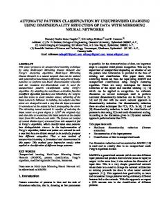
It is used for audio handling. The earlier music classification studies directed us to MFCCs [8] as a methodology to characterize time domain waveforms as little frequency domain coefficients. To process the MFCC, we at first analyze the middle portion of the waveform and took 20ms diagrams at a parameterized break. For independent layout we used hamming window to smooth the points of time. After this, we proceeded with the Fourier change to develop the repeat modules. We then put the frequencies to the Mel scale which models human perspective of changes in pitch, which is generally immediate below 1kHz and logarithmic more than 1kHz. These mapping packs the frequencies into 20 containers by figuring triangle window coefficients in perspective of the Mel scale. Copying these by the frequencies and taking the log we then took the discrete cosine transform, which fills in as a figure of the KarhunenLoeve transform to de-correlate the repeat fragments. Finally, we kept the underlying 15 of these 20 frequencies since higher frequencies are the purposes of point of interest that have a lesser degree an impact to human acknowledgment and contain less information about the melody. Finally, we displayed each uneven tune waveform as a grid of cepstral components where every section is a vector of 15 cepstral frequencies and 20ms plot for a parameterized number of edges per tune (see Fig. 1).

MFCC flow.

be understood if such an inner item can be figured straightforwardly.

ALGORITHMS

A. K-Nearest Neighbour (k-NN) The first machine learning technique we utilized was the k-closest neighbors (k-NN) [5] as it is very famous for its simplicity of execution. The k-NN is by design non-linear and it can detect direct or indirect spread information. It also slants with a huge amount of data. The essential computation in our k-NN is to measure the distance between two tunes. We handled this by methods of the Kullback-Leibler divergence [10]. B. Support Vector Machine (SVM) The second technique we used is the support vector machine [6] which is a directed organization method that discovers the extreme boundary splitting two classes of information. During this the information is not directly distinct in the feature space; if this is the case then they can be put into an upper dimensional space through method of Mercer kernel. Actually, the internal results of the information focuses in this higher dimensional space are essential, so the projection can

The space of potential classifier tasks comprises of biased direct arrangements of key preparation occurrences in this kernel space [41]. The SVM training algorithm selects these weights and support vectors to improve the boundary amongst classifier boundary and training orders. Since training instances are specifically utilized in characterization, utilizing complete tracks as these samples supports very well with the issue of track taxonomy. SVM can be used in direct or indirect strategies once we have an incomplete set of points in various dimensions SVM inclines to be real because it has the capacity to discover the straight separation that should exist. SVM is great with outliers as it will just utilize the most related points to find a true separation. VI.

METHODOLOGY

Before starting, we added necessary toolboxes to the search path of MATLA. These were as follows: 

Utility Toolbox.

340 | P a g e www.ijacsa.thesai.org

(IJACSA) International Journal of Advanced Computer Science and Applications, Vol. 8, No. 8, 2017

 Machine Learning Toolbox.  SAP (Speech and Audio Processing) Toolbox.  ASR (Automatic Speech Recognition) Toolbox. We wrote a script to read in the audio files of the hundred tracks per category and extracted the MFCC features used for individual track. We additionally reduced the dimension of each track because extracted features are based on MFCC’s statistics [8] comprising mean, std, min, and max along respectively dimension. Since MFCC has 39 dimensions, the extracted file-based features have 39*4=156 dimensions. To conclude, we used k-NN and SVM machine learning techniques via compact features set as well as with all features set of each track.

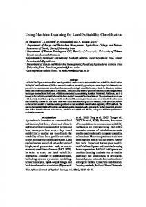
Fig. 2.

Class sizes.

Below is the list of platform and MATLAB version that we utilized as a part of our investigation Platform: PCWIN64.

156 features 1000 instances 10 classes

MATLAB version: 9.0.0.341360 (R2016a)

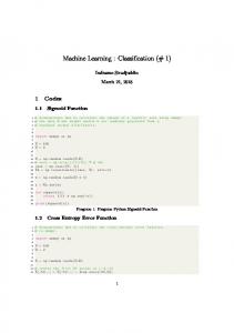
We plotted the range of features of the dataset (see Fig. 3):

A. Data Collection We gather all the sound files from the directory. The sound files have extensions of ―au‖. These files have been sorted out for simple parsing, with a sub folder for each class. Result. Collecting 1000 files with extension ‖D:/szabist/matlab/GTZAN/genres‖...

―au‖

from

B. Feature Extraction For every song, we separated the comparing feature vector for classification. We utilized the function mgcFeaExtract.m (which MFCC and its measurements) for feature extraction. We additionally put all the dataset into a single variable ―dataset‖ which is less demanding for further handling which includes classifier development and assessment. Since feature extraction is extensive, we just loaded the dataset.mat. As discussed above the extracted features are based on MFCC’s, so the extracted file-based features had 39*4=156 dimensions.

Fig. 3.

Features range.

D. Dimensionality Reduction The measurement of the feature vector is very large: Feature measurement = 156.

Result. Extracting features from each multimedia object... 100/1000: file=D:/szabist/matlab/test1/GTZAN/blues/.. 200/1000: file=D:/szabist/matlab/test1/GTZAN/classical/.. 300/1000: file=D:/szabist/matlab/test1/GTZAN/country/.. 400/1000: file=D:/szabist/matlab/test1/GTZAN/disco/.. 500/1000: file=D:/szabist/matlab/test1/GTZAN/hiphop/.. 600/1000: file=D:/szabist/matlab/test1/GTZAN/jazz/.. 700/1000: file=D:/szabist/matlab/test1/GTZAN/metal/.. 800/1000: file=D:/szabist/matlab/test1/GTZAN/pop/.. 900/1000: file=D:/szabist/matlab/test1/GTZAN/reggae/.. 1000/1000: file=D:/szabist/matlab/test1/GTZAN/rock/.. Saving dataset.mat... C. Data Visualization Since we had all the necessary information stored in ―dataset‖, we applied different functions of machine learning toolbox for data visualization and classification. For example, we displayed the size of each class (see Fig. 2):

We considered dimensionality reduction via PCA (principal component analysis) [7]. Initially the cumulative variance gave the descending eigenvalues of PCA (see Fig. 4):

Fig. 4.

Variance percentage vs. No. of eigen values.

341 | P a g e www.ijacsa.thesai.org

(IJACSA) International Journal of Advanced Computer Science and Applications, Vol. 8, No. 8, 2017

A realistic choice is to maintain the dimensionality such that the cumulative variance percentage is greater than the threshold which is 95%. We reduced the dimensionality to 10 to keep 95% cumulative variance via PCA (see Fig. 5).

classification we used a function mgcOptSet.m to put all the Music Genre Classification related options in a single file. Using this classifier, we achieved following result. Training Recognition Rate = 84.69% Validating Recognition Rate = 64.20% The recognition rate is 64%, indicating SVM is a much more effective classifier. We plotted the confusion matrix for better understanding of the results (see Fig. 7). Our experiment showed that if PCA is used for dimensionality reduction, the accuracy will be lower. As a result, we kept all the features for further exploration. Again the k-NN (k-nearest neighbor classifier) was used but with all features. The result was just over 55% which is less then what was achieved before. Result. R = 55.1 % for dataset after input normalization. The confusion matrix was plotted for this in Fig. 6.

Fig. 5.

Features range with reduced dimensions.

E. Classification and Results At first we used the k-NN (k-nearest neighbor classifier) [5] for classification. Result. RR = 52.3 % for original dataset.

Fig. 7.

SVM with reduced dimensions.

RR = 57.6% for original dataset RR = 64.9% for dataset after input normalization Now the recognition rate is improved from 55% to 64% which is equivalent to the previous recognition rate of SVM, it shows that with all features k-NN is more effective classifier (see Fig. 8). Not achieving the satisfied result, we again used SVM but with all features. Result. Fig. 6.

k-NN with reduced dimensions.

After k-NN we used other classifier in order to get a better result hence SVM [9] was used. Before using SVM for

Training RR=99.01% Validating RR=77.00%

342 | P a g e www.ijacsa.thesai.org

(IJACSA) International Journal of Advanced Computer Science and Applications, Vol. 8, No. 8, 2017

So now the training rate is improved from 84.69% to 99.01% and recognition rate is improved from 64% to 77% (see Fig. 9 below).

disco with rock and reggae with hip-hop. The success rate of country was 70% but with rock genre it was just 12%. Hip hop genre had the success rate of 74% but had difficulty differentiating between reggae with highest inaccuracy of 14%. Jazz was identified with the accuracy rate of 90% but had difficulty in recognizing classical genre. Rock has the lowest success rate of 59% having difficulties with many other genres. K-NN had difficulty differentiating between other genres with blues with lowest success rate of 49%. The success rate of rock genre was 62% which was better than the SVM. Overall we found that SVM is more effective classifier which gave 77% accuracy. VIII. FUTURE WORK In the end our study creates a simple solution on the genre classification problem of music. However, it could be further extended out in a few ways. For instance, our research doesn’t give an absolute reasonable correlation between learning strategies for classification of music genre. The exact similar methods utilized in this research could be effortlessly stretched to categorize songs created on some further category, like including extra metadata content elements for example music album, track name, or lyrics. [1]

Fig. 8.

k-NN with all dimensions. [2]

[3]

[4]

[5] [6]

[7] [8]

[9]

Fig. 9.

SVM with all dimensions.

[10]

VII. CONCLUSION Accuracy of classification by different genres and different machine learning algorithms is varied. The success rate of SVM was 83% but the blues genre was misjudged as rock or metal genre. The k-NN did badly while recognizing blues with a recognizing percentage of 49%. The SVM also misidentified classical genre as jazz or hip-hop, but the rock genre was accurately identified with success rate of 94%. The K-NN did also well when identifying classical with success rate of 90%. Similarly, the SVM did also well with recognizing entire categories but on the other hand it also inaccurately identified

[11]

[12]

[13]

[14]

REFERENCES Chathuranga, Y. M. ., & Jayaratne, K. L. (2013). Automatic Music Genre Classificaiton of Audio Signals with Machine Learning Approaches. GSTF International Journal of Computing, 3(2). Serwach, M., & Stasiak, B. (2016). GA-based parameterization and feature selection for automatic music genre recognition. In Proceedings of 2016 17th International Conference Computational Problems of Electrical Engineering, CPEE 2016. Dijk, L. Van. (2014). Radboud Universiteit Nijmegen Bachelorthesis Information Science Finding musical genre similarity using machine learning techniques, 1–25. Aucouturier, J., & Pachet, F. (2003). Representing Musical Genre: A State of the Art. Journal of New Music Research, 32(February 2015), 83–93. Leif E. Peterson (2009) K-nearest neighbor. Scholarpedia, 4(2):1883. Mandel, M. I., Poliner, G. E., & Ellis, D. P. W. (2006). Support vector machine active learning for music retrieval. Multimedia Systems, 12(1), 3–13. Jolliffe, I. T. (2002). Principal Component Analysis, Second Edition. Encyclopedia of Statistics in Behavioral Science, 30(3), 487. Logan, B. (2000). Mel Frequency Cepstral Coefficients for Music Modeling. International Symposium on Music Information Retrieval, 28, 11p. Fu, Z., Lu, G., Ting, K. M., & Zhang, D. (2011). A survey of audiobased music classification and annotation. IEEE Transactions on Multimedia, 13(2), 303–319. West, K., & Cox, S. (2004). Features and Classifiers for the Automatic Classification of Musical Audio Signals. Proc. International Society for Music Information Retrieval Conference, 1–6. Aucouturier, J.-J., & Pachet, F. (2004). Improving timbre similarity: How high’s hte sky? Journal of Negative Results in Speech and Audio Sciences, 1(1), 1–13. Retrieved from Bilmes, J. A. (1998). A gentle tutorial of the EM algorithm and its application to parameter estimation for gaussian mixture and hidden markov models. ReCALL, 4(510), 126. Moreno, Pedro, J., Ho, Purdy, P., & Vasconcelos, N. (2003). A Kullback-Leibler divergence based kernel for SVM classification in multimedia applications. Proceedings of Neural Information Processing Systems, 16, 1385–1393. Li, T. L. H., Chan, A. B., & Chun, A. H. W. (2010). Automatic Musical Pattern Feature Extraction Using Convolutional Neural Network.

343 | P a g e www.ijacsa.thesai.org

(IJACSA) International Journal of Advanced Computer Science and Applications, Vol. 8, No. 8, 2017

[15] [16]

[17]

[18]

[19] [20] [21]

[22]

[23]

[24]

[25]

[26]

[27]

Proceedings of the International MultiConference of Engineers and Computer Scientists (IMECS 2010), I, 546–550. Xu, C., Maddage, N. C., Shao, X., Cao, F., & Tian, Q. (2003). Classification using support machine, 429–432. Meng, A., Ahrendt, P., & Larsen, J. (2005). Improving music genre classification by short-time feature integration. ICASSP, IEEE International Conference on Acoustics, Speech and Signal Processing Proceedings, V, 497–500. Li, T., Ogihara, M., & Li, Q. (2003). A comparative study on contentbased music genre classification. Proceedings of the 26th Annual International ACM SIGIR Conference on Research and Development in Informaion Retrieval SIGIR 03, 15(5), 282. Berenzweig, A., Logan, B., Ellis, D. P. W., & Whitman, B. (2004). A Large-Scale Evaluation of Acoustic and Subjective Music-Similarity Measures. Computer Music Journal, 28(2), 63–76. Liang, D., Gu, H., & Connor, B. O. (2011). Music Genre Classification with the Million Song Dataset 15-826 Final Report. Rhodes, C. (2009). Music Information Retrieval, II(2008), 1–14. Retrieved from http://www.doc.gold.ac.uk/~mas01cr/teaching/cc346/ Tzanetakis, G., & Cook, P. (2002). Musical genre classification of audio signals: IEEE. IEEE Transactions on Speech and Audio Processing, 10(5), 292–302. Logan, B., & Salomon, a. (2001). A Music Similarity Function based on Signal Analysis. IEEE International Conference on Multimedia and Expo 2001, 0(C), 952–955. Gjerdingen, R. O., & Perrott, D. (2008). Scanning the Dial: The Rapid Recognition of Music Genres. Journal of New Music Research, 37(2), 93–100. Lippens, S., Martens, J. P., & De Mulder, T. (2004). A comparison of human and automatic musical genre classification. 2004 IEEE International Conference on Acoustics, Speech, and Signal Processing, 4, iv-233-iv-236. Liu, Z., & Huang, Q. (2002). Content-Based Indexing and Retrieval-byExample in Audio. Proceedings of the 2000 IEEE International Conference on Multimedia and Expo (ICME ’00), 2(c), 877–880. Saunders, J. (1996). Real-time discrimination of broadcast speech/music. Acoustics, Speech, and Signal Processing, 1996. ICASSP-96. Conference Proceedings., 1996 IEEE International Conference on, 2, 993–996 vol. 2. E. Scheirer and M. Slaney, ―Construction and evaluation of a robust multi feature speech/music discriminator,‖ in Acoustics, Speech, and

[28] [29]

[30]

[31] [32]

[33]

[34] [35]

[36]

[37] [38]

[39]

[40]

[41]

Signal Processing, 1997. ICASSP-97., 1997 IEEE International Conference on, vol. 2. IEEE, 1997, pp. 1331–1334. Kimber, D., & Wilcox, L. (n.d.). Acoustic Segmentation for Audio Browsers 1 Introduction 2 Acoustic Segmentation. Boyce, R., Li, G., Nestler, H. P., Suenaga, T., & Still, W. C. (2002). Locating singing voice segments within music signals, (October), 7955– 7956. Foote, J., & Uchihashi, S. (2001). The beat spectrum: A new approach to rhythm analysis. Proceedings - IEEE International Conference on Multimedia and Expo, 881–884. Srinivasan, H., & Kankanhalli, M. (2004). Harmonicity and dynamicsbased features for audio. Proc. ICASSP, 4, 321–324. Zhang, Y., & Zhou, J. (2004). Audio Segmentation Based on MultiScale Audio Classification. IEEE International Conference on Acoustics, Speech, and Signal Processing, 349–352. George Tzanetakis. 2002. Manipulation, Analysis and Retrieval Systems for Audio Signals. Ph.D. Dissertation. Princeton University, Princeton, NJ, USA. Mckinney, M. M. F., & Breebaart, J. (2003). Features for Audio and Music Classification. Proc ISMIR, 4(November 2003), 151–158. Lu, L., Zhang, H. J., & Jiang, H. (2002). Content analysis for audio classification and segmentation. IEEE Transactions on Speech and Audio Processing, 10(7), 504–516. P. Ahrendt, A. Meng and J. Larsen. (2004). Decision time horizon for music genre classification using short time features, 12th European Signal Processing Conference, Vienna, pp. 1293-1296. J. T. Foote, (1997). Content-based retrieval of music and audio, Int. Soc. Opt. Photon. Voice Video Data Commun., pp. 138-147. Li, G., & Khokhar, A. A. (2000). Content-based indexing and retrieval of audio data using wavelets. In IEEE International Conference on Multi-Media and Expo (II/TUESDAY ed., pp. 885-888) Scheirer, E. D. (1998). Tempo and beat analysis of acoustic musical signals. The Journal of the Acoustical Society of America, 103(1), 588– 601. ―Marsyas data sets.‖ [Online]. http://marsyas.info/downloads/datasets.html Available: Accessed on 20th July 2017 Cristianini, N., & Schölkopf, B. (2002). Support Vector Machines and Kernel Methods: The New Generation of Learning Machines. Artificial Intelligence Magazine, 23(3), 31–42.

344 | P a g e www.ijacsa.thesai.org