Automatic Flow Classification Using Machine Learning Isara Anantavrasilp
Thorsten Schöler
Department of Computer Science, Technische Universität Dresden
Corporate Technology, Information and Communications, Siemens AG
[email protected]
[email protected]
Abstract: Network standards are moving toward the Quality-ofService (QoS) networking. Differentiated Services (DiffServ) QoS model is adopted by many recent and upcoming networks standard. Applications running on these networks can specify suitable service classes to their connections or flows. The flows are then treated according to their service classes. However, current Internet applications are still designed based on besteffort scheme and, therefore, cannot benefit from QoS support from the network. An automatic flow classification framework, which can automatically classify non QoS-aware flows or legacy flows, has been proposed in our earlier work [2]. In this paper, we extend our framework by introducing new features that can be effectively used to classify legacy flows. The simplicity of these features allows the data to be collected in real-time. No packetlevel data are required. Furthermore, the framework is evaluated using multiple data sets from different users. The results show that our framework works extremely well in general and it can be operated independently from any applications, networks or even machine learning algorithms. Average correctness up to 98.82% is achieved when the framework is used to learn and classify unseen flows from the same user. Cross-user classifications yield average correctness up to 74.15%.
1. INTRODUCTION Differentiated Service (DiffServ) [5] QoS model is one of the essential features provided by recent network standards such as IPv6, UMTS, WiMAX, IEEE 802.11e, etc. Applications running on these networks can specify “service class labels” to their flows indicating the flows’ QoS requirements. The network can subsequently treat each flow differently based on its service class. However, even though Quality-of-Service support is provided by the networks, current Internet applications are still implemented based on the best-effort scheme. These applications do not specify service classes to their flows and may not be able to benefit from QoS support provided by the networks. These besteffort applications are called “legacy applications”. In [2], an automated flow classification framework is proposed. The framework, assisted by a machine learning algorithm, can automatically classify legacy into appropriate service classes. Because of the self-learning ability, the
framework is independent of any specific sets of application or QoS model and should work in any current or future networks that implement differentiated services or any service class-based QoS schemes. It also aims to provide QoS support for end-user’s legacy applications and is designed to be deployed in the end-device. This would guarantee that the legacy applications will receive QoS support whenever available regardless of whether or not the underlying networks have flow classification facilities. Furthermore, the framework does not rely on any application or protocolspecific characteristics such as packet payload signatures or ports in both learning and classification processes. It is focused only on characteristics that can be observed at network layer [14] such as packet size, throughput, transport layer protocols and connection time. In this paper, we extend our previous work by introducing new features, which can more effectively discriminate the service classes. These features can be calculated in capturing time, eliminating the need to store data per packet and instead requiring storage per flow. Moreover, since the features are calculated on the spot and only a portion of flow data is required, real-time classification (whereby classifications take place shortly after the flow has started) can be archived. We also evaluate our classification framework on data sets from multiple users with diverse networks and applications. The evaluation results show that our methodology works well on the data sets from all users. The new framework achieves average classification correctness of 93.15% - 98.82% when trained and evaluated on the data from the same user. Crossuser evaluations yield correctness of 68.98% - 74.15%. In addition, we evaluate the algorithms in terms of learning time. The results show that, although the algorithms provide similar prediction accuracy, their computational times can vary significantly. The paper is organized as follows. Section 2 discusses current solutions on flow classification. Section 3 describes service classes used in our framework. In Section 4, the flows features and how they are extracted from the data flows are explained. Section 5 examines the framework evaluation strategy as well as the data sets and the evaluation results. Finally, Section 6 concludes the paper.
Table 1 – Observable Features Feature Description Transport Protocol Remote Port Connection Time Traffic (Data Volume, Number of Packets) (Total, Sent, Received, Sent:Received Ratio) Throughput (Data Rate, Packet Rate) (Total, Sent, Received) (Peak / Average / Differences)
2. RELATED WORKS In the context of providing QoS support to legacy flows, many approaches have been proposed [10][19][25][27]. These, however, all rely on user assistance or pre-defined classification rules, which are neither adaptive nor practical. In [24], Roughan et al. use clustering algorithms to classify legacy flows. Nevertheless, due to the nature of these algorithms, large data set might be required in both classification and learning processes [28]. Packet and flows recognition/classification are also important in the network security field. Backdoors detector presented in [30] identifies the malicious services by examining packet payloads for protocol-specific patterns or semantics. This concept is shared by many other works such as [20][21][23]. Elsewhere, machine learning and statistical methods are employed to automatically classify flows based on their behavior without relying on specific patterns or packet payloads [11][29][18][3][4]. Our proposed method is different from the aforementioned approaches in that it does not require huge data sets as in [29][18][3][4] or [24]. Moreover, while some works also require complex data pre-processing before performing classification [30][9][8], our flow classification framework uses only flow-level features that can be captured and calculated in real-time. Unlike [11][20][21][23][30], our framework is also designed to be independent of any applications or networks and can automatically classify flows with unknown protocols. More importantly, despite the simplicity of our features, our experiment results show that they are still remarkably discriminative.
3. SERVICE CLASSES The service classes are defined based on the classes suggested by 3GPP in [1]. However, in order to obtain better characteristic descriptions, we classify the suggested “conversational class” as either strict or relaxed since their service quality requirements are different. • Strict conversational class : Consists of real-time video/audio conferences or real-time online games, such as first-person shooters, which are more sensitive to QoS than other game genres [6][12]. Applications in this class are error-tolerant but sensitive to delay, jitter, and throughput.
Possible Value TCP / UDP TCP/UDP Port Millisecond Bytes / No. of Packets Bytes / No. of Packets
Data Type Nominal Integer Integer Integer / Real Integer / Real Integer / Real Integer / Real
• Relaxed conversational class: Consists of lighter conversational applications, such as Telnet, SSH, remote access, instant messaging, or non-real-time online games, such as strategy or turn-based games. While this class requires less bandwidth and is less sensitive to delay and jitter, they are error-intolerant. • Streaming class: Consists of applications that serve data streams including media streaming and data transfer. We recognize that media streaming and data transfer are fundamentally different in QoS requirements, but they practically exhibit the same behavior [2]. Therefore, we classify them as the same class although it might lead to overestimating the requirement of data transfer flows. • Interactive class: Includes all kinds of server-access applications such as web browsers and email clients. This class is not sensitive to delay, jitter, or throughput. Its main requirement is error-tolerance. Background class is not considered in the framework as legacy applications are designed based on the best-effort scheme and will behave according to their true nature. Thus, there is no true background service in the best-effort scheme.
4. FEATURES Quality-of-Service requirements of each class are typically expressed by four fundamental QoS parameters: delay sensitivity, delay variation (jitter), throughput, and error tolerance (or bit-error rate). However, some of these requirements cannot be observed and measured directly. Therefore, we need to look for other observable features, which can capture the classes’ characteristics and distinguish the classes. Following are the features that should be able to convey the service behaviors and, consequently, be used to discriminate service classes. • Throughput difference: Interactive services are different from streaming services in term of burstiness. Data rate of streaming flows are typically steady whereas the interactive traffic is burstier [9]. However, the burstiness itself cannot be measured directly. In [2], above-mean area and energy are introduced to represent burstiness. Although these are discriminative, they are difficult to calculate and may not be computed in real-time. We thus propose a novel feature – the throughput difference – that can effectively capture the bursty
Table 2 – Data sets and classification correctness of each algorithm on each data set Users User 1 User 2 User 3 User 4
Data set User’s applications Mainly web browsing follows by real-time online games, video streaming, video conference and chat Mainly real-time online games follows by web browsing, chat and streaming respectively Mainly web browsing, follows by video streaming, chat, audio conference, and online games Mainly web browsing, stock ticker, and video streaming, few online games. Average correctness
Correctness of each algorithm (%) PART RIPPER Naïve Bayes
Data Size
J4.8
9364 flows
98.73
98.54
98.46
93.37
7928 flows
97.14
97.98
97.56
89.52
8992 flows
99.31
99.43
99.52
97.73
8191 flows
99.11
99.33
99.32
91.98
98.57
98.82
98.72
93.15
Table 3 – Classification per-class correctness of each algorithm on each data set Class Str. Conv. Rlx. Conv. Streaming Interactive
User 1 99.10 99.18 97.55 99.56
J4.8 User 2 99.56 98.20 95.03 98.14
User 3 100.00 98.41 98.17 99.86
User 4 N/A 72.83 99.53 99.61
Class Str. Conv. Rlx. Conv. Streaming Interactive
User 1 98.88 98.64 97.73 99.50
RIPPER User 2 99.87 98.44 95.38 97.67
User 3 100.00 96.83 98.57 99.76
User 4 N/A 75.00 99.78 99.46
Class Str. Conv. Rlx. Conv. Streaming Interactive
User 1 100.00 98.37 97.38 99.43
PART User 2 99.87 98.55 96.08 97.50
User 3 100.00 96.83 97.88 99.75
User 4 N/A 73.91 99.85 99.61
Class Str. Conv. Rlx. Conv. Streaming Interactive
User 1 92.81 95.65 94.29 97.44
Naïve Bayes User 2 88.44 98.49 85.71 81.79
User 3 98.77 98.41 93.19 98.49
User 4 N/A 82.61 95.08 89.60
behavior. Since throughputs of bursty flows may vary over time, burstiness can be captured by summing these throughput differences over the course of communication. The sum of the throughput differences, denoted
Φ i , is:
n
Φi =
∑φ
i j
− φ ij−1
j =1
i j
where φ is throughput of flow i at calculation window j, n is the number of windows during the capturing time and
φ0i = 0.
Throughput difference consists of data rate and packet rate and into incoming and outgoing directions. Bursty flows should have high sum of throughput differences while steady streaming flows should have low throughput differences. At any rate, the throughput difference depends not only on the burstiness, but also on the overall data volume or the number of packets. Hence, the sum of the throughput difference
Φ i has to be normalized by either of these flow characteristics first. Defining the calculation window as a window of m packets, the throughput is calculated by first measuring the time interval and total data volume between the times at which the first packet and the m-th packet arrive the network interface, and then dividing the volume by the time interval. This way, the flow-wise throughput can be obtained from packet timestamps without maintaining time window for each flow. In the experiments, m is set as 10, as our observations show
that the window of this size is the most suitable to capture the actual throughput peaks and their differences. This is because throughput calculated from a shorter window would not have high enough differences to be measurable while using a longer window would yield near-average throughput, which is not very informative. • Average packet size: As shown in [15], flows from different service classes contain packets of different sizes. Flows in conversational classes typically have smaller packets to achieve high throughput, whereas flows in streaming class usually consist of large packets. Apart from the aforementioned features, other features as listed in Table 1 are employed as well. Note that the transport protocol is only treated as an attribute; it does not matter which protocol is used by the flows. Also, we do not utilize any packet-level information such as packet payload or protocol specific signatures. The features calculation requires only a portion of flow data to be captured. Section 5.1 discusses the flow capturing in details.
5. FLOW CLASSIFICATION In this section, the evaluations of our flow classification framework are described. We will first begin with a description of the data set used in the evaluation, followed by a brief overview of the machine learning algorithms used in
our evaluation, a discussion over the evaluation strategy, and the evaluation results respectively. 5.1 Data Collection and the Data Set Our aim in the present paper is to develop a framework that could be deployed in a user end-device, independently of any specific networks or applications. Therefore, the data used to evaluate the framework must be of a certain degree of diversity. We collected various characteristics of 34,475 flows from four diverse users (see Table 2 for more details). According to [17], the average size of recent web pages is around 130 Kbytes and the traditional modem speed is 56 kbit/s. It would therefore take about 19 seconds to finish downloading an average web page. Thus, capturing time of 30 seconds should be more than enough to differentiate the interactive class from the other classes. This conjecture is supported by our findings that virtually all of the interactive flows last shorter than 30 seconds and that the flow characteristics captured within that duration can adequately distinguish the service classes. Furthermore, because the framework requires only 30 seconds of observation time and the feature values can be calculated at capturing time, the classifications can be done in just 30 seconds from the time the flows started – hence enabling real-time classification. Although shorter flows might not be able to fully benefit from the framework, it does not pose a serious problem since the QoS-sensitive flows such as conversational or streaming flows usually last much longer than 30 seconds. The issue of an optimal observation time will be investigated in our future works. To capture real-world traffics and network usages, the data are collected by letting the users run their usual applications. Our monitoring tool, which runs in the background, will capture and store flows’ statistics automatically. As a consequence, some flows might be running concurrently with other flows (which could belong to other applications) while others might be running alone. The users range from a high school student whose main applications include online gaming and media streaming to an investor who primarily uses stock ticker and web browsing applications. This diversity ensures that the applications, hardware and accessed networks of these users are different. The data were collected and preprocessed by an advanced network monitoring tool: FlowStat. FlowStat first aggregates packets into flows from sequence of captured packets that have the same source IP, source port, destination IP, destination port, and transport protocol. It then calculates flows statistics on-the-fly without storing any packet-level data. Therefore, only the flow-level data are stored, saving considerable space. Nevertheless, we are not concerned about traffic in other network layers as the framework is aimed at end-devices.
5.2 Evaluation Strategy We have investigated a wide range of machine learning algorithms based on different biases, with the main purpose of finding an algorithm that can correctly classify the legacy flows. However, we also seek algorithms whose knowledge representation is intuitive and can be easily interpreted. To this end, we have selected four algorithms to evaluate, namely, J4.8 decision tree [22], PART [13] and RIPPER [7] rule generators, and a basic classifier, Naïve Bayes [16]. J4.8, the decision tree algorithm, takes a top-down approach. It first examines all the features at each level of the tree and then determines which one is the most discriminative in separating the classes at their respective levels. Rules generator algorithms, on the other hand, consider each class individually and try to find rules that cover as many instances of that class as possible, while simultaneously excluding the maximum number of instances from the other classes. Lastly, the Naïve Bayes classifier, which employs Bayes theorem, works by statistically classifying the flows based on background knowledge. The evaluations are conducted in two main phases: singleuser and cross-user. In the single-user phase, machine learning algorithms are applied to the data set from each user to learn the flow behaviors of that user and use the learned knowledge to classify unseen flows from the same user. The accuracy is evaluated using 10-fold cross validation (CV) method [26]. 10-fold CV divides the data set into 10 partitions, trains the learner with the first nine partitions and uses the last one to evaluate the correctness. It then selects another set of different partitions to train and test the learner. The process is repeated until every partition has been used as a test set. The overall correctness is the average accuracy of all iterations. In the cross-user phase, each algorithm is trained using the data from one user but is evaluated on the data from the others. The data sets used in the training and evaluating the learner are called the “training set” and “test set” respectively. 5.3 Evaluation Results Table 2 reports the evaluation results of the first phase where machine learning algorithms are trained and tested by the data from the same user using cross-validation method. Despite the diversities of the users, all algorithms perform significantly well on every data set, with PART performing especially better than other algorithms in most cases. In Table 3, per-class correctness of each algorithm is presented. The results show that the algorithms perform equally well in all classes across data sets, and the overall correctness is not biased by correctness of any particular classes. Note that User 4 has never used strict conversational flows and hence the result for that class is missing.
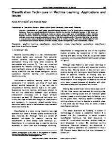
We have also evaluated the algorithms in terms of computational time required to build the classification models (or learning time). In our observations, the classification times of all algorithms are extremely low and not significantly different. Thus, they are not considered here. The tests are performed on a 3.2GHz Pentium 4 with 1GB of RAM running MS Windows XP SP2. Figure 1 shows the average learning time of each algorithm on each of the data sets. Although there is little variation in terms of classification accuracies, as seen from Table 3, huge differences in learning time are observed here. Naïve Bayes learns considerably faster than the other algorithms on all data sets, as it simply collects the flow characteristics. Conversely, because it has to construct and revise the learned rules, RIPPER requires at least twice as much time than the other algorithms. Considering the computational time alone, Naïve Bayes would clearly be the preferred choice, even though its prediction accuracies are still inadequate. J4.8, on the other hand, provides the best trade-off between accuracy and computational time. In any case, the similar prediction results from all algorithms indicate that the features employed by the framework are discriminative. It is thus safe to conclude that our framework is independent not only of the applications or networks, but also of the machine learning algorithms.
Computational Time (seconds)
20
applications. User 2, for instance, regularly plays online games as well as using other applications such as streaming. Learner using the data from User 2 can better classify other data sets than the one from User 4, who usually uses only web browsers. Another reason is that the classification rules are too specific. The flows of the same class from different user, in spite of their similar behaviors, might not be exactly the same. For example, consider the following rule obtained by training PART algorithm on User 1’s data. protocol = TCP AND remote_port