GEOPHYSICS, VOL. 63, NO. 5 (SEPTEMBER-OCTOBER 1998); P. 1696–1707, 15 FIGS.
Automatic NMO correction and velocity estimation by a feedforward neural network
Carlos Calderon-Mac´ ´ ıas∗ , Mrinal K. Sen‡ , and Paul L. Stoffa∗∗
ABSTRACT
We describe a new method of automatic normal moveout (NMO) correction and velocity analysis that combines a feedforward neural network (FNN) with a simulated annealing technique known as very fast simulated annealing (VFSA). The task of the FNN is to map common midpoint (CMP) gathers at control locations along a 2-D seismic line into seismic velocities within predefined velocity search limits. The network is trained while the velocity analysis is performed at the selected control locations. The method minimizes a cost function defined in terms of the NMO-corrected data. Network weights are updated at each iteration of the optimization process using VFSA. Once the control CMP gathers have been properly NMO corrected, the derived weights are used to interpolate results at the intermediate CMP locations. In practical situations in which lateral velocity variations are expected, the method is applied in spatial data windows, each window being defined by a separate FNN. The method is illustrated with synthetic data and a real marine data set from the Carolina Trough area.
INTRODUCTION
Artificial neural networks (ANNs) have been applied successfully in several areas of science and engineering, such as handwriting recognition, speech recognition, and signal detection (e.g., Freeman and Skapura, 1991; Cichocki and Unbehauen, 1993). Their application in exploration geophysics has been rather limited. They have been mainly applied to problems that involve the recognition of characteristic patterns in measured data. An example of this is first-break picking from seismic data (Murat and Rudman, 1992; McCormack
et al., 1993) or velocity picking from velocity scans for velocity analysis (Schmidt, 1992; Fish and Kasuma, 1994). Other ANN applications include the location of subsurface targets using electromagnetic field data (Poulton et al., 1992), the study of shear-wave splitting from two horizontal component seismograms (Dai and MacBeth, 1994) and the characterization of reservoirs from seismic reflection data (An and Moon, 1993). The ANN architecture adopted in all of these applications is the multilayer feedforward neural network (FNN). The FNN is the most widely used ANN to solve pattern recognition problems because of the simplicity of its implementation and its generality for solving a variety of problems. A FNN consists of neurons or processing units arranged in successive layers with connections between neurons of one layer to the following layer and with no connections between neurons within the same layer (Figure 1). In this layer arrangement, data flow in one direction starting from the first layer or input layer. The operational characteristics of the network are primarily controlled by a set of weights or connection strengths that map an input pattern into an output pattern, usually through a nonlinear expression. In a FNN, weights are commonly computed from minimizing the difference between the network output once the input pattern has been propagated through the network, and a desired output. The process of finding a set of weights that will produce a least-squares fit between computed and desired output is known as the backpropagation training method; the input-output patterns used for training are known as the training set. The purpose of learning a mapping between known input-output patterns is to later apply the trained network to input patterns with unknown outputs. From this viewpoint, a FNN is simply a nonlinear function, and the training process an optimization problem where network weights are the parameters to be estimated. Current approaches to velocity analysis based on ANNs (Schmidt, 1992; Fish and Kasuma, 1994) use the interpreter’s experience to provide a set of examples for FNN training in the
Presented at the 66th Annual International Meeting, Society of Exploration Geophysicists. Manuscript received by the Editor April 18, 1997; revised manuscript received February 4, 1998. ∗ Formerly Department of Geological Sciences and Institute for Geophysics, The University of Texas at Austin; presently Mobil E&P Technology Center, P.O. Box 650232, Dallas, TX 75265. E-mail: carlos
[email protected]. ‡Institute for Geophysics, The University of Texas at Austin, 4412 Spicewood Springs Road, Building 600, Austin, TX 78759-8500. E-mail: mrinal @utig.ig.utexas.edu. ∗∗ Department of Geological Sciences and Institute for Geophysics, The University of Texas at Austin, 4412 Spicewood Springs Road, Building 600, Austin, TX 78759-8500. E-mail:
[email protected]. ° c 1998 Society of Exploration Geophysicists. All rights reserved. 1696
Automatic NMO Correction by a FNN
1697
form of velocity picks from a velocity spectrum . The inputs of the FNN correspond to semblance values from the velocity spectrum picked by the interpreter. The desired output of the FNN is a one or zero value that acts as a yes/no classifier that validates the picks. The network is trained until it is able to mimic the picks provided by the interpreter. Once adequately trained, the FNN is used as an automatic procedure for interpreting velocity spectra. This approach to automatic velocity picking does not include a physical model for relating the semblance values to the picked velocities. In this work, we present a new method for automatic NMO correction and velocity estimation using a FNN that avoids the training process through experience and is more directed toward an unsupervised method. The input data for the FNN are τ - p transformed common midpoint (CMP) gathers at selected control locations along a 2-D seismic line. The network outputs are interval velocities at those locations. Network training involves minimizing an objective function defined in terms of NMO-corrected data. During training, network weights are updated based on a global optimization method known as very fast simulated annealing (VFSA). The final output of the training process are the control CMP data properly NMO corrected. Once the network has been trained, the computed weights can operate on new CMP gathers that lie between the selected control locations, thus saving interpretation time when processing large data sets. The proposed approach to network training is not restricted to the NMO-correction and velocity estimation process, but it can be adapted to other problems such as prestack migration velocity analysis. We illustrate the method with synthetic data and a real marine data set from the Carolina Trough area.
first layer and sequentially proceeding to the remaining layers (Diebold and Stoffa, 1981; Shultz, 1982), the interval velocity of each layer can be estimated and its effect removed from the underlying layers. Assuming a medium consisting of laterally homogeneous layers, NMO correction in the τ - p domain can be computed using the following equation (Diebold and Stoffa, 1981):
DESCRIPTION OF THE METHOD
where M is the number of p-traces, N the number of time samples, yk represents the p = 0 trace or target trace at sample k obtained from averaging a small number of traces at the beginning of the gather, and xik the ith NMO-corrected trace for the same time sample. A good correction should align in phase all traces with the target trace. Since the main objective is to obtain velocity-time functions from the NMO corrections, differences in amplitude are not considered by the method. Dynamic amplitude equalization is applied to the data as part of the data preprocessing. Also, for preserving only subcritical reflections in the evaluation of the objective function, an upper limit for the propagation angle defines a mute zone. The method described here performs NMO correction for a group of CMP gathers. Based on equation (2), the total error from NMO-correcting a group of Q CMPs is defined as
NMO correction in the τ -p domain When seismograms are transformed to the intercept time and ray parameter domain (τ - p domain), reflection events including supercritical reflections are organized into elliptical trajectories. In a medium consisting of homogeneous layers, only the first event maps into a true ellipse, the underlying layers map into pseudo-ellipses. Based on an operation that involves removing p-dependent time shifts starting with the
¡ ¢1/2 1τk ( p) = 1τk (0) 1 − p 2 vk2 ,
where vk is the interval velocity of layer k, and 1τk (0) is the two-way normal traveltime for the same layer. Equation (1) describes an elliptical curve in the τ - p domain for layer k. If interval velocities as well as two-way normal times for each of the layers are known, we can remove the angle-dependent time shift 1τk ( p) starting from the first layer and sequentially proceeding with the remaining layers, resulting in a layer stripping operation. In this work, the cylindrical slant stack τ - p transformation method (e.g. Treitel et al., 1982) is applied to convert CMP gathers to the τ - p domain. The criterion to find the velocity-time function that gives a good correction is to search along several elliptical trajectories [i.e., time-shifts in equation (1)] for maximum coherence. The measure of coherence used in this work is the L1-norm harmonic measure (Porsani et al., 1993):
2 h1 = 1 −
N M X X
|yk − xik |
i=1 k=1 N M X X
|yk + xik | +
i=1 k=1
E =1−
FIG. 1. Two-layer feedforward neural network.
(1)
N M X X
,
(2)
|yk − xik |
i=1 k=1
Q 1 X h 1i . Q i=1
(3)
The error measure of equation (3) is optimized to obtain the group of velocities that correct the observed data the best. The final velocities obtained by the method should be considered as parameters that produce optimum alignment of primary reflections on the traces of the CMP gathers, which may not be the true propagation velocities. Only for the case of flat horizons and homogeneous layers can the resulting velocities be considered estimates of true interval velocities. The presence of dipping horizons, for example, introduces errors in the velocity estimates in direct relation to the degree of the dip (Diebold
1698
Calderon-Mac´ ´ ıas et al.
and Stoffa, 1981), but the computed velocities can still be used for moveout calculation and stacking. A discussion related to the differences that exist between stacking velocities obtained from NMO correction and true interval velocities can be found in the works of Taner et al. (1970) and Schneider (1971), and a description of the factors that affect these differences is given by Al-Chalabi (1974).
Feedforward neural networks A FNN has one or more hidden layers of neurons between the input and the output layers of the network. The inputs to one neuron in a hidden layer come from the previous layer and its outputs go to the next layer, hence the term feedforward. The number of hidden layers and the number of neurons per hidden layer necessary to accomplish successful learning are problem dependent and are typically obtained through experimentation. For most FNN applications, a single hidden layer would produce as good a result as defining the FNN with more than one hidden layer. Assuming that we have a set of Q input data vectors (x1 , x2 , . . . , xq , . . . , x Q ) each having L elements, we want to train a FNN (such as the one shown in Figure 1) to approximate an output for each of the input vectors. The interaction of the jth single neuron of a hidden layer of H neurons with input data vector xq is given by
à q aj
L X
= f
! q w ji xi
+ bj ,
(4)
i=1 q
where a j is the net response of the jth neuron to the q input vector, j = 1, 2, . . . , H, L denotes the number of samples of the input vector, w ji is the ith weight of neuron j, and b j is a translation term of function f . In a similar manner, the output layer of the FNN is given by
à q ok
= gk
H X
! q wk0 j a j
+ ck ,
(5)
j=1 q
where ok is the kth output of the FNN, k = 1, . . . , S, where S defines the number of output parameters to estimate, wk0 j is the jth weight of neuron k in the output layer, and ck is the kth translation term of function gk . Functions f and gk in equations (4) and (5) represent the activation functions of the network. In the neural network context, the activation function can take several forms. One that is used commonly is the nonlinear sigmoid (S shape) function,
f (x) =
1 − exp(−2αx) , 1 + exp(−2αx)
(6)
where α is a parameter that controls the steepness of the function near x = 0. A sigmoid function has the important characteristics that its first derivative is always positive and that its range is asymptotically bounded. Although the forms of f and gk are the same for equations (4) and (5), they have different bounds. For the hidden layer, the output of the sigmoid function is confined within −1 and 1. For the network output, the search limits of parameter m k define the limits of the sigmoid
function, or in other words
¡ ¢ gk (x) = 12 [ f (x) + 1] m max − m min , + m min k k k
(7)
where m max and m min correspond to the maximum and minik k mum search limits, respectively. Equations (4) and (5) are used to compute an output for each of the input vectors x. In the following section, we will describe how to obtain the weight matrices w and w0 . ˜ ˜ Automatic NMO correction by a FNN The input data of the FNN are τ - p–transformed CMP gathers at selected control locations in a seismic line. The number of input elements of a single training example is given by the number of p-traces and the number of samples per trace (L = M × N ). Network weights and sigmoid activation functions map the input data into interval velocities, the network outputs. Velocities can be described by a fixed number of layers of known two-way normal traveltime, by spline coefficients, or by some other smooth representation. The number of velocity layers or spline coefficients used to define the 1-D velocity-time functions gives the number of neurons S in the output layer of the network [equation (5)]. The limits of the activation functions in the network output are given by the search limits of each output parameter. Weights are first initialized with random numbers between −1 and 1. Once a set of input vectors have been mapped by the FNN to network outputs, a velocity-time function per input vector, the data are NMO corrected and the error evaluated using equation (3). Notice that the error is not obtained directly from the FNN output but from the NMO-corrected data. The computation of network weights is now cast as a nonlinear optimization problem, and we introduce the ideas of the simulated annealing algorithm (e.g., Rothman, 1985; Sen and Stoffa, 1995) for weight updating. In simulated annealing, model parameters are perturbed based randomly on previous model parameter evaluations (weights, in the case of a neural network). A control parameter known as temperature drives the minimization toward the most promising parts of the cost function. The temperature is lowered during the optimization process according to a cooling schedule. The cooling process works in a way that the likelihood of accepting a model with a higher error than the current model is higher at the beginning of the process. As cooling continues, this likelihood decreases and, at the end of the optimization, only models with a lower error than the error from the current model are accepted. We use this acceptance criterion for weight updating. At this point, we describe a method to perturb weights that is based on the VFSA method first introduced by Ingber (1989). A detailed description of VFSA and how it differs from the standard simulated annealing algorithm is in Sen and Stoffa (1995). VFSA has the property that model parameter wi j at iteration ` is obtained from its value at a previous iteration according to the equation
w`ji = w`−1 ji + r ji 1w,
(8)
where 1w = w max − wmin , wmax and w min correspond to limits fixed previous to minimization, wmin ≤ w `ji ≤ w max for all ( j, i), and r ji ∈ [−1 1] is a random number. We use [−1 1] for the
Automatic NMO Correction by a FNN
weight limiting values. VFSA uses a product of Cauchy-like distribution functions for generating the random number r ji . A random number u ji drawn from a uniform distribution U [0, 1] can be mapped into this distribution using the formula (Ingber, 1989)
¶ "µ ¶|2u ji −1| # 1 1 r ji = sgn u ji − T` 1 + ` , 2 T µ
(9)
where sgn is the sign function and T ` is the temperature parameter at iteration `. A high value of T ` at the beginning of the process allows us to sample with equal probability the entire search space of each weight being perturbed, while for low values of T ` weight perturbations tend to zero. Constraining at each iteration the sampling for each of the weights results in fewer rejected models than the standard simulated annealing method. Cooling of the temperature in VFSA is defined by the equation
T ` = T 0 exp[−β(` − 1)1/2 ]
(10)
where T 0 is the initial temperature and β is a positive number close to 1.0 from the left that controls the decreasing rate of the cooling curve. In the general case, the starting temperatures and cooling curves for the acceptance rule and that of equation (9) differ. In this work, we use a similar temperature schedule and initial temperature for both parameters. Optimum cooling parameters are obtained from experimentation. Typical parameters for the starting temperatures and decay rates of the cooling curve are 1.0 and 0.97, respectively. Once the output velocities produce the best alignment of the reflections in each CMP gather, final network weights are used
1699
to NMO-correct CMP gathers at intermediate locations with the FNN acting as a velocity interpolator. Figure 2 shows flow charts describing the general procedure for automatic NMO correction using a FNN. The number of control CMPs required by the method for successful training and prediction are dependent on the complexity of the data being processed. We have found from experimentation that using a FNN with a hidden layer of 15–22 neurons and trained with 10–25 control CMP gathers produces good training and prediction results. Velocity search limits are defined based on a priori information on the velocity field. Velocity search limits of 1–2 km/s are considered in the examples below. APPLICATION OF THE METHOD
Synthetic data experiment First, we test the method using synthetic data generated from the velocity model shown in Figure 3. The model consists of six layers and a reflector geometry characterized by an anticline of gentle slopes encased in low velocity layers. The first layer of the model has a velocity of 1.5 km/s; while the other layers have a constant background velocity to which a high-frequency random perturbation, with 0.2 km/s as the maximum perturbation, has been added. The same perturbation is applied throughout the model (reflectors are continuous). The velocity model is 4 km in the horizontal direction and 3 km in the vertical direction. Velocities range between 1.5 and 4.2 km/s. The grid sizes are 0.02 and 0.01 km in the horizontal and vertical directions, respectively. The model shown in the figure has been transformed from depth to time for comparison purposes since velocities are estimated in time. Multiple-free synthetic data were computed using a Kirchhoff summation method and an acoustic finite-difference
FIG. 2. Flow chart of the automatic NMO-correction method using FNNs.
1700
Calderon-Mac´ ´ ıas et al.
eikonal traveltime solver based on the work of Faria and Stoffa (1993) following the work of Schneider et al. (1992). Sources and receivers are located at every grid point at the surface of the model. A Ricker wavelet with 22 Hz of central frequency and zero phase was used as the source wavelet. The time sampling interval is 8 ms. The model was extended 1 km at the extremes following the subsurface geometry at the edges to produce CMP data of 50 trace fold with a trace separation of 0.04 km and offsets between 0 and 2 km. The CMP gathers were transformed to the τ - p domain using the slant-stack τ - p–transformation method. Each CMP gather was trans-
formed to 21 traces with 0.02 s/km of spacing between traces for a maximum ray parameter of 0.4 s/km. Figure 4 shows five CMP τ - p gathers for different locations along the model. In the first experiment, 11 CMP gathers regularly spaced by 0.4 km were input to a FNN with 15 neurons in the hidden layer. A 0.5-s dynamic amplitude gain correction (AGC) was applied to the data for evaluating coherence after the NMO corrections. The outputs of the network are cubic spline coefficients fixed in time and regularly spaced between 0.4 and 2.0 s at every 0.2 s, resulting in eight spline coefficients per training example. Velocity search limits were approximately 1.7-km/s
FIG. 3. Velocity model plotted in time. A velocity log is shown at the middle of the model.
FIG. 4. CMP synthetic τ - p data.
Automatic NMO Correction by a FNN
wide for each model parameter and centered approximately around the true velocity at the center of the model. Water depth and the velocity of the first layer were assumed known. The FNN was trained using VFSA for 2000 forward modeling evaluations (NMO corrections) of the 11 training examples. Figure 5 shows the error curve obtained during network training.
FIG. 5. Training history generated from NMO-correcting 11 CMP gathers.
1701
After training, reflection events in the control CMP gathers align in phase correctly. Applying the trained network to CMPs at the intermediate location should produce similar results. Figure 6 shows CMP groups that have been NMO corrected with the trained network (top) and the estimated velocities for each of the groups (bottom). Only the CMP gather located at 2.0 km was part of the data used for training. The trained FNN produces good NMO-corrected data and, in general, the final velocities follow the true velocities, except for the gather at 3.9 km that shows overcorrection. This CMP gather is located at the extreme of the model, where layers have the most pronounced dip, indicating that a denser sampling of the training examples may be required in this part of the model. To improve these results, two control CMP gathers at the extremes of the model were added, reducing by half the spacing between the control CMP gathers. Network weights from the previous experiment were used as the starting point for training the FNN for 500 iterations, reducing the starting temperature by half. Interpolation results with the trained FNN are presented in Figure 7. All groups are now nearly perfectly NMO corrected, and the estimated velocities produce a better match with the true velocity, indicating that splines produce a good average velocity model for NMO correction and stacking. The final estimated velocity field is presented in Figure 8.
FIG. 6. NMO-correction results for five CMPs (top). True (dashed) and estimated (solid) velocities are shown for each of the CMP gathers (bottom); the shaded area corresponds to the velocity search range.
1702
Calderon-Mac´ ´ ıas et al.
FIG. 7. Improved NMO-correction results after adding four examples for training from the edges of the model.
FIG. 8. Final velocity model from NMO correcting 100 CMPs using the trained FNN.
Automatic NMO Correction by a FNN
1703
The estimated velocity can be interpreted as a parameter that produces optimum processing results. The degree of bias of this parameter from the true velocity is related to the lateral variations of the velocity model (as well as to nonrandom interference such as multiple energy, but this is not considered here). The problem is more pronounced when lateral velocity anomalies have dimensions of the order of a CMP spread, thus causing the moveout curve to differ from true ellipses. Still, a best-ellipse fit would be found by the method, but this may yield incorrect estimates of the velocity. This could be corrected by iterative modeling using ray tracing or by prestack depthmigration analysis. Here, the emphasis of the proposed method is to obtain NMO-corrected data that produce a good stack section. Figure 9 shows the final stack section. In this figure, the trained network was used to interpolate 100 CMP gathers, one at every 0.04 km, using 15 of those examples for network training. Once trained, the network is able to interpolate results at any location along the line. In other words, knowledge of the velocity distribution is somehow stored in the weights of the network. The number of control locations for adequate training depends, as observed in this experiment, on the complexity of the data. The use of many examples for training and wide parameter search limits will result in exhaustive training. Figure 10 shows a comparison of error histories when training a FNN with 11 control CMP gathers that sample the entire model and when training the network with seven CMP gathers regularly spaced between 2.8 and 4.0 km. Both networks use the same parameter search limits. The network trained with fewer examples converges to a good solution in approximately half the number of iterations than the network trained with 11 examples. This shows that for practical purposes, it may be simpler to consider several FNNs which may be defined with different velocity search limits trained with different parts of the seismic line than to train a single network for processing the entire line. A second approach to the problem is to use a single FNN that is applied as a sliding spatial window with data overlapping in the successive windows. This approach has the benefit that the network weights computed for one window can be used as the starting point for the next window, reducing the total training time.
Real data example
FIG. 9. Final stack section obtained by NMO-correcting CMP gathers every 0.04 km using the computed weights from the FNN trained with 15 examples.
FIG. 10. Comparison of error histories when training a FNN with 15 examples distributed along the entire model (solid) and with seven examples from a part of the model (dashed).
In a second experiment, the method was tested with a surface marine seismic data set from the Carolina Trough off the East Coast of the United States. The University of Texas Institute for Geophysics collected the data set in 1988 as part of a deeppenetration seismic program. The data were acquired with a 6.25-km-long streamer with 240 receivers with a 0.275-km distance between the source array and the first receiver group. The separation between shots was 0.05 km, and the record length was 16 s sampled at 0.004 s. Previous studies with these data addressed crustal studies (Oh et al., 1991) and a bottom-simulated reflection (BSR) anomaly related to the presence of methane hydrate in shallow sediments (Wood et al., 1994). Based on the high signal quality of the data and the long streamer used in the acquisition, Varela et al. (1998) performed velocity analysis for these data using a migration misfit criterion (MMC) and a reflection tomography criterion (RTC) with data organized in common offset sections. Part of line BA-6 was selected for testing the automatic NMO-correction method. The data were first organized in CMP gathers with a 240-trace fold and a trace separation of 0.025 km with offsets between 0.275 and 6.25 km. The separation distance between CMP gathers was 0.050 km. The part of BA6 used for the test consists of CMPs 1850−2130 (14 km). Only the first 6 s of the record length were used to test the NMO-correction method. As part of the processing of the data, spiking deconvolution and multiple attenuation based on differential moveout filtering in the f -k domain were applied to the data before the τ - p transformation. In addition to this, an internal mute of near-offset traces contaminated by the first multiple from the water column was also applied. The CMP data were transformed to 41 p-traces with pmax = 0.4 s/km and a trace separation of 0.01 s/km. Every other p-trace in each transformed CMP gather was used as input of the FNN. Since the p = 0 trace is not accurately obtained from the transformation, a stack of the first three ray-parameter traces was used to define the target trace. Figure 11 shows the near trace gather section. The section shows two distinct primary reflections and the first water-related multiple. Figure 12 shows a CMP gather after processing, and its τ - p transform pair.
1704
Calderon-Mac´ ´ ıas et al.
NMO correction was performed with three FNNs. The first network was trained with 20 control CMP gathers from 0 to 5 km and 0.25-km spacing between control gathers. The second and third networks were trained with 18 examples each from 5 to 9.5 km and from 9.5 to 14 km, respectively, with a 0.25-km spacing. The velocity model for each of the control CMP locations was parameterized with eight spline coefficients fixed in time at every 0.5 s. Velocity search limits were 1.0 km/s wide for the shallow part and approximately 1.8 km/s for the deepest part of the model. Higher velocities were used for the first FNN
(0–5 km), the other two FNNs (5–14 km) used the same velocity search limits. The water bottom was fixed for each control location, and a propagation velocity of 1.5 km/s was assumed for the water layer. Figure 13 shows the velocity search limits and the spline node locations for each of the FNNs. Each FNN had 15 neurons in the hidden layer and was trained for 3000 iteration. The number of training-control CMP gathers including the three networks was 56. Once trained, the networks were used to NMO-correct 280 CMP gathers that comprise the selected seismic line. Figure 14 shows NMO-
FIG. 11. Near trace section from the Carolina Trough data set.
FIG. 12. Typical CMP gather from line BA6 (left) and its τ - p transform (right).
Automatic NMO Correction by a FNN
1705
FIG. 13. Velocity search limits used for automatic NMO correction for the fist FNN (left) and second and third FNNs (right). Circles indicate the location of the spline nodes. correction interpolation results for three groups of five CMP gathers each. These groups are located at the middle of the control CMP locations selected for each of the trained networks. The first and last CMP gathers in each of the groups correspond to training examples, the CMP gathers between these groups correspond to interpolation results. The trained networks produced acceptable NMO corrections for both the training CMP gathers as well as for the intermediate locations. The final stack section is presented in Figure 15, which shows an improved signal quality when compared to the near trace section. The performance of the network along the profile depends on the differences in the signal quality between training groups and interpolated groups. For the Carolina Trough data, using control CMP gathers at every 0.2 km gave nearly perfect NMO corrections. With half the number of control locations used for training, the NMO-correction results degraded for part of the seismic section (from 0 to 5 km). DISCUSSION AND CONCLUSIONS
The usefulness of applying FNNs to the problem of NMO correction and velocity analysis is presented. Most applications of ANNs in geophysics have been for problems in which a FNN is trained to learn a relationship between input-output corresponding patterns. For the seismic velocity analysis problem, this would mean deriving velocity-time or velocity-depth functions from seismic gathers. Unfortunately, this straightforward approach is not practical since, in the analysis of field seismic data, we rarely have an accurate set of known answers (seismic velocities) to train the network with. Correspondingly, it is almost impossible to generate a synthetic data set with the characteristics of real data for network training. The FNN-based NMO-correction and velocity analysis method presented here avoids the requirement of having a set of known velocity models for training. This is accomplished by training the FNN while NMO-correcting some CMP gathers at selected locations. Rather than employing the commonly used error criterion that is based on computing the differences between the predicted and known velocity models, the error
is calculated based on the goodness of NMO correction of the data themselves. This method completely avoids the traveltime or velocity picking based on interpreter experience used by other approaches to the problem. An interpreter’s intervention is required only to select the control locations for FNN training and the velocity search limits that define the limits of the sigmoid output functions. The central idea of the method is that the weight update process is based on data error. Weights are not directly related to the network computation, thus error can be defined in several ways. Network training is performed with VFSA. In this method, weight updates are obtained from previous iterations and are temperature dependent. Synthetic as well as real data experiments show that, after training, weights produce an estimate of the velocity which performs NMO corrections quite well. ACKNOWLEDGMENTS
C. Calderon-Mac´ ´ ıas thanks the National Council of Science and Technology of Mexico ´ (CONACyT) for its support. This research was supported by National Science Foundation grant EAR-9304417. REFERENCES Al-Chalabi, M., 1974, An analysis of stacking, rms, average and interval velocities over a horizontally layered ground: Geophys. Prosp., 22, 458–475. An, P., and Moon, W. M., 1993, Reservoir characterization using feedforward neural networks: 63th Ann. Int. Mtg., Soc. Expl. Geophys., Expanded Abstracts, 138–141. Cichocki, A., and Unbehauen, R., 1993, Neural networks for optimization and signal processing: John Wiley & Sons, Inc. Dai, H., and MacBeth, C., 1994, Split shear-wave analysis using an artificial neural network: First Break, 12, 605–613. Diebold, J., and Stoffa, P. L., 1981, The traveltime equation, tau-p mapping, and inversion of common midpoint data: Geophysics, 46, 238– 254. Faria, E. L., and Stoffa, P. L., 1993, Traveltime computation in transversely isotropic media: Geophysics, 50, 272–281. Fish, B., and Kasuma, T., 1994, A neural network approach to automated velocity picking: 64th Ann. Int. Mtg., Soc. Expl. Geophys., Expanded Abstracts, 185–188. Freeman, J. K., and Skapura, D. M., 1991, Neural networks: AddisonWesley Publ. Co. Ingber, L., 1989, Very fast simulated annealing: Math. Com. Modeling, 12, 967–993.
1706
Calderon-Mac´ ´ ıas et al.
FIG. 14. NMO-correction interpolation results obtained from training three FNNs. The separation distance between CMP gathers in each group is 0.05 km. The CMP gathers at the extremes of each group correspond to control CMP gathers used for training. McCormack, M. D., Zaucha, D. E., and Dusheck, D. W., 1993, Firstbreak refraction event picking and seismic data trace editing using neural networks: Geophysics, 58, 67–78. Murat, M. E., and Rudman, A., 1992, Automated first arrival picking: A neural network approach: Geophys. Prosp., 40, 587–604. Oh, J., Phillips, J. A., Austin Jr., J. A., and Stoffa, P. L., 1991, Deeppenetration seismic reflection images across the southeastern United States continental margin, in Meissner, R., Brown, L., Durbaun, H. J., Franke, W., Fuchs, K., and Seifert, F., Eds., Continental lithosphere: Deep seismic reflections, 22, Am. Geophys. Union, 225–240. Porsani, M. J., Stoffa, P. L., Sen, M. K., Chunduru, R. K., and Wood, W. T., 1993, A combined genetic and linear inversion algorithm for seismic waveform inversion: 63rd Ann. Int. Mtg., Soc. Expl. Geophys., Expanded Abstracts, 692–695.
Poulton, M. M., Stenberg, C. E., and Glass, C. E., 1992, Location of subsurface targets in geophysical data using neural networks: Geophysics, 57, 1534–1544. Rothman, D. H., 1985, Nonlinear inversion, statistical mechanics, and residual statics estimation: Geophysics, 50, 2784–2796. Sen, M. K., and Stoffa, P. L., 1995, Global optimization methods in geophysical inversion: Elsevier Science Publ. Co., Inc. Schmidt, J., 1992, Neural network stacking velocity picking: 62th Ann. Int. Mtg., Soc. Expl. Geophys., Expanded Abstracts, 18–21. Schneider, W. A., 1971, Developments in seismic data processing analysis (1968–1970): Geophysics, 36, 1043–1073. Schneider, Jr., W. A., Ranzinger, L. A., Balch, A. H., and Kruse, C., 1992, A dynamic programming approach to first arrival traveltime computation in media with arbitrarily distributed velocities,
Automatic NMO Correction by a FNN
1707
FIG. 15. Final stack section obtained after NMO-correcting CMP gathers with the trained networks as velocity interpolators. Fifty-six CMP gathers were used for training.
Geophysics, 57, 39–50. Schultz, P. S., 1982, A method for direct estimation of interval velocities: Geophysics, 47, 1794–1810. Taner, M. T., Cook, E. E., and Neidell, N. S., 1970, Limitations of the reflection seismic data; lessons from computer simulations: Geophysics, 35, 551–573. Treitel, S., Gutowski, P. R., and Wagner, D. E., 1982, Plane-wave de-
composition of seismograms: Geophysics, 47, 1375–1401. Varela, C., Stoffa, P. L., and Sen, M. K., 1998, Background velocity estimation using nonlinear optimization for reflection tomography and migration misfit: Geophys. Prosp., 46, 51–78. Wood, W. T., Stoffa, P. L., and Shipley, T. H., 1994, Quantitative detection of methane hydrates through high resolution seismic velocity analysis: J. Geophys. Res., 99, 9681–9695.