) 1 i-1
3
The problem with formula [2.2] is that the whole rule has to be executed in order to compute it. To solve this problem we will first transform the formula to a form that uses averages rather than the particular values.
Σ COST(Pib)
b∈SOL()
= SOL()
[COST(Pib)]
MEAN
i-1
=∏
SOL()
j=1
Incorporating [2.2] and [2.3] into [2.1] yields: COST()
i-1 = ∑ ∏ i=1 j=1 n
[2.2]
b∈SOL()
MEAN SOL(P j b )
[2.3]
b∈SOL()
[2.4]
MEAN SOL(P j b ) ∗ MEAN [ COST(Pib)] b∈SOL() b∈SOL()
The next step is to find a good approximation of [2.4] that can be computed without computing the whole rule. Given a subgoal P i, instead of taking the mean over all the bindings generated by the previous subgoals, we will use the mean over a superset of Pi. The superset will be the Calling Pattern for Pi. The calling pattern is defined after [3] , but we use a binary domain, with the elements ground and nonground, while [3] uses a more sophisticated domain with four elements (empty, closed, free and don't know). Definition: Given a goal P(t1,...,tn) where t1,..,tn are already substituted under the current binding, the calling pattern for that goal is P(C(t1),...,C(tn)) where C(ti) ∈ {0,1}. C(ti)=1 iff ti is a ground term under the current substitution. Thus, for example, the calling pattern of the goal parent(john,Y) is parent(1,0). As mentioned in [3], the reason for using such patterns is to approximate the unbounded number of literals, that may appear while proving a query, by a finite set of equivalence classes. Having such a finite set will enable us to collect various statistics needed for the ordering process (for example, cost and number of solutions). We do not claim that calling patterns are the best partition possible, and further research should be done to explore the possibility of more sophisticated classification of the arguments (possibly using semantic information). Given a database with M predicates, the number of possible calling patterns is
∑2 M
ARITY(Pi)
i=1
The learning program will consider only a small subset of the calling patterns - those encountered during the training phase. Let P be a goal and a sequence of goals. Let CP(P,) be the calling pattern of P assuming all variables of P which appear in are bound. Let COST(cp) and NSOLS(cp) be the means for the cost and number of solutions for the calling pattern cp computed after solving a set of problems. The modified formula for the approximated cost is: [2.5] n i-1 COST()= ∑ ∏NSOLS(CP(Pj,)) i=1 j=1
4
∗ COST(CP(Pi,))
LASSY, the system described in the next section, builds a table of costs and number of solutions for the calling patterns, and uses this table to estimate the cost of subgoal sequences using formula [2.5].
4. LASSY: a System that Learns domains represented by logic programs. The basic terms of the cost equations (and thus the ordering procedure) are the averages of costs and number of solutions for the various calling patterns. How may these averages be obtained? Naish [13] suggested collecting statistics to estimate the number of solutions to calls to database procedures "over some period of typical usage". But what is "typical usage"? This question is part of a set of problems that LASSY as well as many other learning systems have to face. LASSY is a system that learns domains represented by Prolog databases, and exploits domain specific knowledge to accelerate the search process of the interpreter. The system has both a deductive learning component and an inductive learning component. The inductive component is described in this paper. The deductive learning component, the lemma learner, which is outside the scope of this paper, is described in [9, 11]. The design of the LASSY system assumes that the Prolog interpreter receives tasks (queries) from an external source, and that the main goal of the system is to improve the expected average speed with which the interpreter will execute future tasks. It is also assumed that the system performs off-line learning (i.e. no learning takes place while solving externally supplied problems) and that learning time is "cheaper" than performance time. LASSY's main learning method is "learning by doing": the system learns while doing tasks of the same type that the performance system does (Prolog queries in our case). We assume that there is no external agent that provides training problems to the system, thus the system must be able to generate its own problems. The self-generated tasks must be informative, i.e. they should lead the system to acquire useful knowledge. The next subsection describes the architecture of LASSY which was designed to satisfy the assumptions and solve the problems discussed above. This architecture can be generalized to many other learning systems that satisfy those assumptions. 4.1. System architecture The performance element of LASSY is a POST-Prolog interpreter [10]. POST-Prolog is a simple extension of Prolog that allows the programmer to specify which parts of programs should be executed in particular order and which parts can be executed in any order that the system wishes. POST-Prolog is described in the appendix. There are two main data structures that the learning system maintains: 1. The task model - a representation of the prediction of the learning program of the set of future tasks. LASSY currently uses a weighted set of query templates as its task model. 2. The domain model - the main product of the learning process. The acquired knowledge that will be used by the Prolog interpreter in order to improve performance. LASSY maintains a table of average cost and number of solutions for calling patterns.
5
The learning system employs two major learning procedures. The first is the main learning module that updates and maintains the domain model (we call it primary learner). The primary learning process is performed in the following way. First the task generator generates queries using the task model as a guide. Then the POST-Prolog interpreter proves the queries under the primary learner control. The primary learner observes the interpreter during the problem solving and updates the domain model. The second learning procedure creates and updates the task model (we call it the secondary learner). The secondary learner gets as input the set of queries the system has received from external sources, and updates the task model. The architecture of LASSY is illustrated in figure 1.
Past tasks
Solutions
Interpreter
External tasks
(under external control)
Domain model (costs and #solutions)
Task model learner
Primary learner
Task model
Solutions
Task generator
Interpreter Training tasks
(under learner control)
Figure 1 4.2. The task model The task model expresses the system's beliefs about the types of tasks it is going to be facing in the future. In LASSY, as in most learning systems, it is assumed that the tasks it receives are drawn randomly from a space with a fixed distribution. If the task stream that the problem solver faces is drawn from a population with fixed distribution, why can't the system just use the past tasks as training tasks ? It can - if it has enough of them. The task model enables the system to generate as many tasks as needed for trainingwithout depending on tasks from external sources. The task model built and maintained by LASSY is based on the concept of calling patterns that was mentioned in Section 2. A task model is a weighted set of problem templates together with a set of predicate domains. A problem template is a calling pattern: a predicate symbol followed by a sequence of 0's and 1's. For example, ((ancestor 0 1) 17) is the pattern for queries that ask for ancestors of a specified person and its weight is
6
17 (a problem of this type will be generated with probability of 17/total-weight). For each predicate that appears in the problem templates, the task model contains a list of the predicate domains. A predicate domain is a set of ground terms. The task model builder receives as an input a set of queries that were given to the system in the past. For each query, the procedure checks to see whether its calling pattern is in the model. If it is in the model, the weight associated with it is incremented, otherwise it is added to the model. To generate a problem from the task model, a problem pattern is selected with probability proportional to its weight. Then a query is generated by selecting a random member of the appropriate domain for each of the required ground arguments . 4.3. The domain model Most of the cost and number of solutions information of ground predicates (predicates whose clauses are all ground) can be retrieved by scanning the database and counting. Thus, before the learning program is engaged in its learning-by-doing process, it accumulates the statistics about the ground clauses - their number, and the sizes of the domains of their arguments. We call term this process static learning. Averages that can not be collected by the static learning process are acquired through a the dynamic learning phase. LASSY performs dynamic learning by continuously generating queries using the task model and updating the domain model while solving the queries. The domain model is a table with an entry for each predicate. Each entry contains average information for the predicate regardless of the calling pattern and an entry for each calling pattern encountered during learning. Each such entry contains counters for the number of times that a subgoal matching the calling pattern was invoked, for the total cost of executing the subgoal, and for the total number of solutions so that the average information can always be retrieved from the table. When the interpreter is working under learning system control, it updates the entries in the table. Whenever a subgoal is called, the appropriate entry for the calling pattern is created if necessary, and the calling counter is incremented. Whenever a solution is generated, the solution counter is incremented. Whenever backtracking from a subgoal occurs, the subgoal tree's cost is added to the total cost. The cost of searching the tree of a subgoal is computed in the following way: whenever the interpreter creates a node, its cost is set to zero. Whenever the interpreter tries to unify a goal with a head of a clause, the costs of all the nodes in the path to the root are incremented by 1. Whenever a new subgoal is pushed onto the computation stack, the number-of-solutions counter of the former subgoal is incremented by 1. An entry in the table may look like: ((ancestor 0 1) 27 93 16782) which means that a subgoal with the predicate ancestor, with the first argument unbound and the second argument bound, was invoked 27 times, has generated 93 solutions and had a total cost of 16782 unifications. Thus the average cost for that calling pattern is 621.55 unifications and the average number of solutions is 3.44.
5. Ordering Finding optimal ordering is generally an NP complete problem. Exhaustive search will involve evaluation of N! sequences for N subgoals in the worst case. The work described in this paper deals only with ordering of subgoals within a rule body. A more complete system
7
could allow ordering of all current subgoals within the computation stack. However, the number of possible orderings would be so high that it would not be feasible. In the next section we will give a precise definition of the space searched for an optimal ordering. The states are the partial sequences, and the final states are complete sequences. 5.1. The search space definition Given a set of subgoals P = {P1,...,Pn}, we can define a search space SP = where: S
=
{ {Pj ,..,Pj } ⊆ P} 1 k 1 k
is the set of states.
O:S → 2S is the operator.that generates successor states and is defined as O() = { Pt ∈ P - {Pj ,..,Pj }} 1
k
1
k
1
k
Si
=
is the initial state
Sf
=
{ {Pj ,..,Pj } = P} is the set of final states. 1 k 1 k
g(s1,s2) = NSOL(s1) * COST(s2) is the cost of moving from state s1 to state s2 ∈ O(s1). Given such a space we can perform an A* search to try and find the path with minimal cost. We need to associate with each state the g value (which is a requirement of the A* algorithm), the number of solutions for the subsequence, and the binding pattern for the subsequence (i.e. which of the clause's variables is bound). Thus, when applying the operator to get the successor states we have to calculate the new g, the new number of solutions, and the new binding pattern. 5.2. Pruning the search The problem with an exhaustive search is that in the worst case, it can expand n! nodes. If the search procedure reaches two states that consist of exactly the same set of subgoals (but in different order, otherwise it would be considered the same state), the state with the higher g value can be removed from the set of states that are candidates for expansion, since there is no way that the state with the higher can be a part of the optimal ordering. That prunes the number of states that can be expanded to 2n in the worst case. Smith and Genesereth [5, 19] proved the Adjacency Theorem which reduces substantially the space of possible orderings that should be searched to find an optimal ordering. The theorem was proved in the context of optimizing a conjunctive query in a database consisting entirely of positive ground literals (this type of problem is called "Sequential constraint satisfaction" in [5]). An interesting question is whether the Adjacency Theorem applies also in the case where an execution of a subgoal can carry an arbitrary cost. Unfortunately, the answer is no. To prove it we will show a counter example to one of the corollaries of the theorem. The corollary says: Given a conjunct sequence of length two, the less expensive conjunct should always be done first [5]. The reader should note that "less expensive" in this context means "smaller number of solutions." Assume that we have a set of two conjuncts {P1,P2} that we want to order. For
8
simplicity, assume that P1 and P2 do not share variables. Assume that P1 has 100 solutions, and has a search tree that costs 10000. Assume that P2 has 2 solutions and has a search tree that costs 10. COST() = 10000 + 100*10 =11000 COST() = 10 + 2 * 10000 = 20010 Thus we have a case where the most expensive conjunct should be done first. In practical problem spaces we have found that the the number of nodes expanded is much smaller than 2n . The main reason is that there is a big difference between optimal ordering and many non-optimal orderings: there are many cases where the set of subsequences that are more expensive than the complete optimal sequence is large. The search procedure will never expand such states. The fact that many times n is small also helps to reduce the size of the search. 5.3. Heuristics Finding a good heuristic function for evaluating the minimum cost of moving from the current state to the final state (the h component in the A* terminology) could make the search much faster. The problem is that such a heuristic is hard to find. Using the obvious transformation to the Traveling Salesman Problem, each city will be mapped to a subgoal and the task of finding a path with minimal cost between the cities maps into the task of finding an ordering with minimal cost. Several heuristics have been developed for solving TSP [17]. However, there is one difference that makes the ordering problem "harder" than the TSP - the cost of getting from one "city" to another can only be known when visiting that "city", and it depends on the path that was used to get there. That difficulty makes most of the heuristics used in the TSP useless for a search for optimal ordering. We have implemented the following simple heuristic: given a state s, h(s)=NSOLS(s) * MIN COST(CP(Pi,s)) Pi∈P - s
The above heuristic function is an underestimate of the actual cost. One could claim that this is an advantage, since A* is admissible when h gives an underestimate [15]. However, the size of the search space suggests that admissibility is less important than reducing search time. The problem with the function h defined above is that it is not a very "informed" one (Nilsson [15] defines the relation "more informed" between two heuristics functions - function h1 is more informed than function h2 if h1 always gives better estimate than h2). However, even after relaxing the admissibility constraint, we could not develop a better heuristic. 5.4. Resource bound search Although we have claimed that the time that will be spent on the search will be much lower than the worst case, we need something more substantial to make the ordering worthwhile. The whole idea of the ordering was to invest time in the ordering process itself in order to save greater time from the execution of the goal. If we don't have any reasonable bound on the search time, how can we make sure that we do not actually lose by performing the ordering?
9
The answer is to perform resource bound search. The search procedure will be given as a parameter the amount of resources it is allowed to use. The units for specifying the resources are number of nodes expanded. Given a set of subgoals of size N and a limit of M resources, the search procedure will conduct an A* search until either a solution is found or the number of nodes expanded is M - (N - Length(s)), where s is the current best node, and length(s) is the number of elements in the subsequence of s. The system then proceeds with hill climbing search - that is, it expands the best node, then the best of its successors, and so on. If we use the g function as our evaluation function, then the hill-climbing search is similar to the cheapest first heuristic (except that here we mean cheapest in terms of cost and not in terms of number of solutions). The resource limit given to the procedure is the cost recorded for the calling pattern before using ordering. This is the maximal cost that the ordering procedure can save. The ordering procedure subtract a fixed amount of resources from its given limit to account for the fixed overhead of using the procedure. This method is an example of selective utilization [9, 11]- the system uses a filter to reduce the probability of harmful usage of the acquired knowledge by the problem solver . 5.5. Implementing the ordering procedure The estimated average costs and number of solutions can be retrieved from the inductive knowledge base, but what will the ordering procedure do if there is no entry for a specific calling pattern? In such a case the ordering procedure calls a function that tries to estimate the averages based on various heuristics. Those heuristics set low bounds and high bounds on the value. If, for example, the average is known for a calling pattern that is more general than the current calling pattern (i.e. never has a 1 in a location where the other has 0), we can designate it as a high bound on the current average. The opposite is true for less general patterns. In addition, the procedure uses some other heuristics which will not be discussed here. The ordering procedure caches the ordering results, thus avoiding the need to search again for the best ordering of the same rule with the same calling pattern. The cache is erased whenever any learning occurs because it may not be valid any more.
6. Experimental results The domain used for the experiments is a Prolog database that specifies the layout of the computer network in our research lab. It contains about 40 rules and several hundred facts about the basic hardware that composes the network and about connections between the components. The database is used for checking the validity of the network as well as for diagnostics purpose. The only type of learning that was used in these experiments is the inductive learning described here. All other learning mechanisms (lemma learning) were turned off for the whole duration of the experiments. An experiment consisted of the following steps: 1. A set of 20 random queries was generated using the task model; This is the test set. 2. With all learning turned off, ordering turned off, and using random ordering, the system executed the test set and the performance of the system was recorded. 3. The system performed the static learning - i.e., it scanned the databases to collect information about ground clauses.
10
4. With learning turned off, and ordering turned on, the system performed the test set. In the graph, this point is marked as the test for 0 learning examples. 5. With learning turned on, and ordering turned on, the system generated 10 random queries using the same model and executed them. 6. With learning turned off and ordering turned on the system performed the test set. 7. Steps 5 and 6 were repeated 5 times.
12000
Random ordering
Unifications
10000 8000
Static learning
6000 4000 2000 0 0
10
20
30
40
50
Learning Tasks
Figure 2. The results of the experiment are summarized in figure 2. The Y axis specifies the mean number of unifications taken over the results of the test (i.e. 20 queries). The first observation that we can make is that the best performance (after learning 20 examples) is 10 times faster than the performance with no learning at all. A second observation is that the performance after executing 20 learning tasks is 5 times faster than the performance with ordering that used only the knowledge gathered during the phase of static learning (i.e. the statistics about the ground clauses). The last observation that we make is that the LASSY did not improve its performance while performing the last 30 learning tasks. The reason for this flattening is that after performing 20 examples, the averages approached their final values, thus the ordering procedure always produced the same output. One final comment about the experiment. To finish the experiment in a feasible time, a limit of 20,000 unifications per query execution was set. During the performance of the test with random ordering, the execution of half of the queries was halted after 20000 unifications. Thus, the actual improvement in performance should be much higher than 10 times.
7. Future Research In [18] we have argued that one of the reasons for having the learning system generate its own experiences is that generation of informative experience requires knowledge of the
11
current state of the system's own representation (which is not available to an external agents). Our current scheme of generating training problems does not take advantage of this knowledge. The system will devote a large part of its learning resources to a class of problems that is given very often by external users even if it already knows everything that needs to be known about solving such problems. A future implementation of the task generator will also make use of an internal model of the system. The system will keep a test set drawn from its task model. Occasionally, the system will perform tests and update its performance graphs for all the problem classes. Flattening of the graph (like that shown in figure 2) will indicate that the averages used for this class of problems have approached their final values, and the system will devote more resources to other problem classes. Another feature that we would like to add to the system is the ability to use its learned knowledge with other Prolog systems. We are now building a procedure which will output a transformation of the POST-Prolog program that will be executable in other Prolog environments. The procedure will order the expensive rules for various calling patterns, and will output a set of output rules for each input rule. The output rules will use the standard meta-logical system predicates var and novar to make the interpreter execute the rule with the right order.
8. Conclusions The LASSY system, which was described in this paper, was built in order to make Prolog more declarative by moving the burden of ordering subgoals from the user to the system. Existing systems trying to perform similar tasks had several limitations that could not be solved with the approaches they have taken. LASSY takes a different approach by employing machine learning methods to accumulate the information needed for the ordering program. The system acquires the knowledge by performing self generated training tasks. It ensures the relevance of the knowledge by generating training problems that are similar to past problems received from users. The system performs resource bound A* in order to make sure that the cost of the search for good ordering will not outweigh its benefits. The experiments done showed that the machine learning approach is very promising. With ordering, the system showed an improvement by a factor of 10 compared to performance with random ordering. It would be interesting to compare the results with optimal ordering, but it would be prohibitively expensive to perform the test on all possible orderings in order to find the best one. It is also very often the case that there is no single best ordering, but different orderings are best for different bindings of the rule's head. LASSY can handle such cases with no problems.
Appendix: POST-Prolog: a Partially Ordered Prolog interpreter The Prolog interpreter used as the performance element of the LASSY system is a POST-Prolog interpreter (Partially Ordered STructured Prolog). POST-Prolog is a simple extension of standard Prolog. Its main goal is to allow the programmer to tell the interpreter what parts of the program should be interpreted in a procedural way (i.e. the interpreter has to follow the control specified by the programmer) and what parts should be interpreted in declarative way (the interpreter should supply the control).
12
POST-Prolog adds to the syntax of standard Prolog two pairs of symbols: {,} and . Clauses that are enclosed in {,} can be matched in any order, whereas clauses that are enclosed in should be matched in the order they appear. The same rule applies to subgoals - subgoals enclosed in {,} can be executed in any order, whereas subgoals enclosed in should be executed in the order that they appear. The brackets can be nested to any level. Thus, POST-Prolog changes the semantics of Prolog - in standard Prolog a program is an ordered set of clauses, but in POST-Prolog a program is a partially ordered set of clauses. In standard Prolog a rule body is an ordered set of subgoals, but in POST-Prolog a rule body is a partially ordered set of subgoals. The main idea behind POST-Prolog is that in typical use of Prolog, especially as a database language, the programmer usually wants to specify the control in a few parts of the program (for example, when calling system predicates with side effects, or when writing a recursive procedure). In the rest of the program the programmer does not care about the specific order that clauses will be matched or subgoals will be executed. The problem is that the programmer has no way of telling the system what parts of the program can be reordered by the system. Writing the program down implicitly specifies the control. POST-Prolog is different from other extensions of Prolog (like IC-Prolog [2] and MUProlog [13]). Whereas those extensions involve adding control facilities to standard Prolog, POST-Prolog reduces the amount of control that must be specified by the user, such that the proportion between the part of the control component that is defined by the user and the part of the control component that is supplied by the system is flexible, and can be determined by the user. A more detailed account of POST-Prolog is given in [10]. Acknowledgements The authors wish to thank Bob Kass, Marcial Losada and Kristina Fayyad for comments on earlier drafts of this paper. 1 The original name of the system was SYLLOG. Due to a conflict of names with a system by Walker we have changed the name to LASSY (Learning And Selection SYstem). References
[1]
Brodie, M. L. and Mattias, J., On Integrating Logic Programming and Databases, in: L. Kerschberg (eds.), Expert Database Systems, The bengamin/Cummings Publishing Company, Menlo Park, California, 1986.
[2]
Clark, K. L. and McCabe, F., The Control Facilities of IC-Prolog, in: D. Michie (eds.), Expert Systems in The Microelectronic Age., University of Edinburgh, Scotland, 1979.
[3]
Debray, S. K. and Warren, D. S., Automatic mode inference for logic programs, J. Logic programming 5:207-229 (1988).
[4]
Gallaire, H. and Minker, J., Logic and Data Bases, Plenum, New York, 1978.
[5]
Genesereth, M. R. and Nilsson, N. J., Logical foundations of artificial intelligence, Morgan Kaufmann, Palo Alto, California, 1988.
[6]
Kowalski, R. A., Logic for Problem Solving, Elseveir North Holland, New York, 1979.
[7]
Kowalski, R. A., Directions for Logic Programming, in: Proceedings of IEEE Symposium On Logic Programming, 1985.
13
[8]
Lloyd, J. W., Foundations of Logic Programming, Springer-Verlag, 1984.
[9]
Markovitch, S. and Scott, P. D., Information filters and their implementation in the SYLLOG system, in: Proceedings of The Sixth International Workshop on Machine Learning, Ithaca, New York, 1989.
[10]
Markovitch, S. and Scott, P. D., POST-prolog: Structured Partially Ordered prolog, TR CMI-89-018, Center for Machine Intelligence, Ann Arbor, Michigan, 1989.
[11]
Markovitch, S. and Scott, P. D., Utilization Filtering: a method for reducing the inherent harmfulness of deductively learned knowledge, in: Proceedings of The Eleventh International Joint Conference for Artificial Intelligence, Detroit, Michigan, 1989.
[12]
Mitchell, T. M., Utgoff, P. E. and Banerji, R., Learning by Experimentation: Acquiring and Refining Problem-Solving Heuristics, in: R. S. Michalski, J. G. Carbonell and T. M. Mitchell (eds.), Machine Learning : An Artificial Intelligence Approach, Tioga, Palo Alto, California, 1983.
[13]
Naish, L., Automatic control for logic programs, J. Logic programming 3:167-183 (1985).
[14]
Naish, L., Prolog Control Rules, in: Proceedings of IJCAI, Los Angeles, 1985, pp. 720722.
[15]
Nilsson, N. J., Principles of Artificial Intelligence, Tioga, Palo Alto, CA, 1980.
[16]
Parker, S. D., et al., Logic Programming and Databases, in: Proceedings of Expert Database Systems - Proceedings From the First International Workshop, 1986, pp. 3548.
[17]
Pearl, J., Heuristics : intelligent search strategies for computer problem solving, Addison-Wesley, 1984.
[18]
Scott, P. D. and Markovitch, S., Uncertainty Based Selection of Learning Experiences, in: Proceedings of The Sixth International Workshop on Machine Learning, Ithaca, New York, 1989.
[19]
Smith, D. E. and Genesereth, M. R., Ordering Conjunctive Queries, Artificial Intelligence 26:171-215 (1985).
[20]
Sterling, L. and Shapiro, E., The Art of Prolog, MIT Press, Cambridge, MA, 1986.
[21]
Warren, D. H. D., Efficient Processing of Interactive Relational Data Base Queries Expressed in Logic, in: Proceedings of Seventh International Conference on Very Large Data Bases, 1981.
[22]
Zaniolo, C., Prolog: A Database Query Language for All Seasons, in: L. Kerschberg (eds.), Expert Database Systems, The bengamin/Cummings Publishing Company, Menlo Park, California, 1986.
14