Automatic Parallel Program Generation and Optimization from Data

Proceedings 1991 International Conference on Parallel Processing

Automatic Parallel Program Generation and Optimization from Data Decompositions Edwin M. Paalvast, Henk J. Sips*, A.J. van Gemund TNO Institute of Applied Computer Science (ITI-TNO) P.O. Box 226, NL-2600 AE Delft, The Netherlands *Delft University of Technology P.O. Box 5046, NL-2600 GA Delft, The Netherlands

abstract Data decomposition is probably the most successful method for generating parallel programs. In this paper a general framework is described for the automatic generation of parallel programs based on a separately specified decomposition of the data. To this purpose, programs and data decompositions are expressed in a calculus, called Vcal. It is shown that by rewriting calculus expressions, Single Program Multiple Data (SPMD) code can be generated for shared-memory as well as distributed-memory parallel processors. Optimizations are derived for certain classes of access functions to data structures, subject to block, scatter, and block/scatter decompositions. The presented calculus and transformations are language independent. 1.

Introduction

In programming either shared- or distributed-memory parallel computers, programmers would like to consider them as being uni-processors and supply as little extra information as possible on code parallelization and data partitioning. On the other hand, maximum speed-up is desired, without loss of portability. This trade-off is reflected in the existence of a variety of parallel language paradigms, which, regarding to the decomposition method, can be divided into two categories: implicit and explicit. Languages based on implicit descriptions, like functional [Hudak88, Chen88] and dataflow languages [Arvind88], leave the detection of paral lelism and mapping onto a parallel machine to the compiler. Unfortunately, contemporary compilers do not pro duce efficient translations for arbitrary algorithm-machine combinations. Most languages based on explicit descriptions specify parallelism c.q. communication and synchronization as integral part of the algorithm. This has the disadvantage that one has to program multiple threads of control, which are generally very hard to debug. Hence, experimentation with different versions of the same parallel algorithm, for example different decompositions, is in general rather cumbersome. Comparably small changes may require major program restructuring. An alternative approach is to automatically generate parallel programs in SPMD (Single Program Multiple

1

Data) [Karp87] format, given a data decomposition specification. This approach has recently gained a lot of attention. It has been applied by [Callahan88, Gerndt89, Kennedy89,90] for applications to Fortran, by [Andre90] to C, by [Rogers89] to Id Nouveau, by [Koelbel90] to Kali-Fortran, by [Quinn89] to C*, and by [Paalvast90] to the fourth-generation parallel programming language Booster. In particular application to Fortran shows some limitations, due to equivalencing, passing of array-subsections to subroutine calls, etc. A second limitation is that the description of complex decompositions and especially dynamic decompositions, i.e. a redistribution of the data at run-time, is not feasible either. An exception is [Kennedy89] where a method is presented to describe redistribution. However, this method still has the drawback that redistribution statements are not generated automatically and are intermingled with the program code, which limits portability. A more fundamental problem to these approaches is that distinctive formalisms are used for the description of algorithm and decomposition. Hence, a unified formal system to reason about optimizing transformations at compile-time is not possible. Furthermore, the approaches do not address the issue in the general context of data representation. This paper aims at presenting a language independent framework for representing and reasoning about the transformations involved, yielding a unified and generalized approach to this subject. The approach is based on a so called view calculus, denoted as V-cal. From this several optimizations are derived for important classes of data decompositions. It is shown that parallel programs can be generated for shared-memory as well as distributed-memory parallel processors. 2. 2.1

Program Representation and Transformation

Algorithms and Programs In order to describe program transformations from data decomposition specifications in a language independent way, we need to define which characteristics are to be extracted from a program source code. A first observation is that most algorithms suitable for parallelization involve many identical operations on (parts of) large datastructures. In traditional imperative languages this is reflected

Proceedings 1991 International Conference on Parallel Processing

by implementations involving many iterations over some nested loop-structure, whereas in functional languages the operations are recursively defined over one or more list structures. A second observation is that algorithms can either be described by a function mapping of a set of input values to a set of output values, where the calculations of the output values are mutually independent, or by a function mapping where some values from a previous function application are part of the input set. The first type of mapping is involves no intermediate state and is therefore inherently parallel. The second type of mapping involves some intermediate state and inhibits a sequential component. Note that all algo rithms can be transformed to the first category. However, this can lead to an excessive duplication of work and data. Usually, the use of intermediate states comes quite naturally (e.g. in algorithms exposing obvious complexity when writing them explicitly or algorithms containing intermediate tests on data values). In principle, the state-less part of an algorithm can be expressed in a single expression of the type A=expr(B), where A is a variable and B is a set of variables, representing multi-dimensional data structures, on which an expression expr is defined. Over this expression the sequential part of the algorithm can be defined (if existent). In this paper, we restrict ourselves to datastructures, where the index to the data can be defined by an ordered index set, i.e. a finite set of d-tuples in N, from here on simply called index set. This includes all array-like structures, but excludes relational structures like trees.

The vector l and u are called the lowerbound and upperbound of the set, respectively, b the bound vector, and the positive integer d the dimension of Nb . ❏ Example 1. The set {(2,3), (2,4), (3,3), (3,4)} is within the bounded set l=(2,3), u=(3,4), but also within the bounded set l = (1,0), u = (8,7). The first bounded set is called a normalized bounded set.

2.2

In general, instead of i, a function prescription will be enclosed between the square brackets: [ip(i)]. The function ip(i) is called the index propagation function. Example 3. Let ip(i) = (i1 +1, i2 +1), then (i1 , i2 )=(1,3), when applied on the index set of the above example, returns the index (2,4).

V-cal In order to capture the essential algorithmic information from programs and be able to perform transformations on those programs, we have developed a calculus, called V-cal. The calculus is constructed around the notion of and manipulation with bounded index sets and uses concepts from set- and function theory. In this paper, only a short introduction is given to V-cal, which should be sufficient to understand the concepts. For a more detailed description, the reader is referred to [Paalvast91b].

2.3

Index Sets The notion of an index set is crucial to V-cal. All transformations and optimizations are expressed in terms of index set manipulations. First we define the notion of a bounded set. Definition 1: The bounded set Nb , with b = (l,u) is given by the Cartesian product N1 ×..×Nd , where l = (l1 , l2 , ..., ld) and u = (u1, u2 , ..., u d ), with l,u ∈Nd , and N i ⊂N is defined as: N i = { n i | li ≤ ni ≤ ui }

i = 1..d

2

Using the bounded set we define an index set as: Definition 2: An index set I is a bounded set Nb , on which a predicate function P: Nc → T is defined. The set I is defined as a set comprehension: I = {i ∈ N b | P(i)} or shorthand I = (b, P).

❏ Example 2. Consider I = (b, P), with l=(0,0), u=(2,2), and P((i 1 ,i2)) = i1 ≤i2 yields the set {(0,1), (0,2), (1,2)}. We will also use the notation I = (0:2×0:2, P), whenever convenient. Next, we define a selection function on an index set I, which selects a single index from I: Definition 3: The single index selection function, denoted as [i], selects the i-th index when applied to I. The application is written as [i](I). ❏

In practice, we often need to be able to express a set of such single index selections, yielding what we call a view. Definition 4: A view V is a onto and one-to-one relation V ⊆ I×J, described by the tuple (K, dp, ip), where I, J, and K are index sets, ip is an integer total function from J to I, and dp is a monotonic increasing function on the bounding vectors of the index set. A view is denoted as √(K, dp, ip), A view application to an index set I is denoted as √(K, dp, ip)(I) = ∆(i ← J) ◊ [ip(i)] (I)

Proceedings 1991 International Conference on Parallel Processing

where it holds that J = (bK & dp(bI), ( PI° ip) ∧ PK), with I = (bI, PI). The parameter expression ∆(i ← J) ◊ binds the index set J to the parameter i, where the symbol ◊ denotes the partial ordering on the elements of J. The '&' operator denotes the bound vector of the intersection of two sets represented by bound vectors. ❏ The parameter expression ∆(i ← J) ◊ can be thought of as an abstract loop, generalizing all forms of DO-loops, such as DOALL and DOACROSS. An important characteristic of views is that they can be composed: Definition 5: The view composition U = V°W is defined by the following compositions on the respective views V = √ ( (bKv, PKv), dpv, ipv), and W = √((bKw, PKw ), dpw, ipw),: ipu = ip w ° ipv dpu = dpv ° dpw bu = bKv & dpv(bKw) Pu = PKw° ipv ∧ PKv

∆(i←J)◊[ip(i)](V⊕W)= ∆(i ← J) ◊ ([ip(i)](V)+[ip(i)](W)). Where ⊕ is the multi-dimensional equivalent of the scalar +. Finally, views can be defined over clauses. Clauses incorporate view expressions and assignments and define state-to-state transformations. For example, ∆(i←J)◊[ip(i)](U:=V⊕ W)= ∆(i ← J) ◊ ([ip(i)] (U) :=[ip(i)](V)+[ip(i)](W)). So far, nothing has been said about the ordering operator ◊. This operator can define arbitrary orderings, of which two forms, ◊ = • and ◊ = //, are of specific importance. The '•' order implies the lexicographical ordering of selections and '//' denotes the absence of such an ordering, implying the possibility of parallel execution.

❏ A derived result of this definition is the so-called contraction of parameter expressions ∆(i ← I) ◊ [ip1 (i)] ∆(j ← J) ◊ [ip2 (j)]. We can write them as the composition √1(I, id, ip1 ) ° √2(J, id, ip2 ) where J = (b,R) and id is the identity function. Then according to Definition 5 this composition is equal to √(I ∩ (b, R°ip1 ), id, ip2 ° ip1 ), which is again equal to the parameter expression: ∆(i ← I ∩ (b, R°ip1 )) ◊ [ip2 (ip1 (i))]. Example 5: We illustrate the principle of view composition with an example: Let

ture A. Predicates on index sets might even be related to data values. For example, [i](A>0) denotes a predicate on i, selecting only those indices of which the associated data values are larger than 0. In the same way, views can be defined over expressions involving multi-dimensional operations. Multi-dimensional operations in V-cal are defined strictly element-wise, according to reduction rules like:

V = (bv, Pv, dpv, ipv,): bv, = (0,1), Pv(i) = {i ≥ 1}, dpv(i) = i – 2, ipv(i) = i + 2 W = (bw, Pw, dpw, ipw): bw = (0,10), Pw(i) = {i ≥ 4}, dpw(i) = i div 2, ipw(i) = 2. i

2.5

Transformation of Programs into V-cal. The question that arises when introducing a new formalism, is the applicability to, for example, existing languages like Fortran or C. To perform this transformation, it is necessary, to a certain extend, to extract the actual algorithm from a given program. This process is far from trivial and may only be partly successful. However, it is shown in [Paalvast90,91b], that the high-level language Booster is can make full use of, and can be translated almost directly to V-cal . In this respect,V-cal presents a model of computation to which restructuring efforts of Fortran and C can be directed, and which, if restructuring is successful, yields the advantage of the rewrite-rules of the calculus. This will be an area for future research. Below we will only give a trivial example of a translation of an imperative program to V-cal (A and B are independent)

The V ° W = (bv°w,Pv°w,dpv°w,ipv°w) : bv°w = (0,1) & (–2,10–2) = (0,1), Pv°w(i) = {i ≥ 4}° ipv ∧ {i ≥ 1}= {i ≥ 2}, dpv°w(i) = (i div 2) – 2, ipv°w(i) = 2. (i + 2) = 2 . i + 4.

for i:=imin to imax do if A[i]>0 then A[i]:= B[f(i)]; fi; od;

2.4

∆(i ← (k+1: n | [i]A>0 ) // ([i](A) := [f(i)](B))

Views on Data Sets, Expressions, and Clauses So far, views are applied to index sets. In reality, a data value of a certain type is related to each index value, similar to an array in conventional languages and its associated index set. From now on, instead of applying a view V to an explicit index set I, e.i. V(I), we will write V(A), denoting the application on the index set IA of a datastruc-

3

Fig.1 Example program and corresponding V-cal expression.

Proceedings 1991 International Conference on Parallel Processing

2.6

Data Decomposition Data decomposition in V-cal can be expressed quite easily. In the sequel, we consider the data structures A and B used in an algorithm as views on the (distributed) memory of a machine. Furthermore, by following the convention that the processor responsible for a certain data element is also responsible for the computations involved in its calculation, we can generate SPMD programs. Consider the following general template, where we restrict ourselves, for reasons of clarity, to the following one-dimensional clause, where A and B have index sets (0:n–1) and (0:m–1): ∆(i ← (imin:imax)) ◊ [f(i)]A :=Expr([g(i)](B))

(1)

If A is replaced by a general decomposition V(A'), with index set (0:pmax–1× 0:k), where A' is the 'machine' image of A, we obtain the following general decomposition view: V=√(K,dp,ip), where K = Ø, dp((l,u))=l*u, ip(j)=(procA(j), localA(j))

p to the left, while causing the condition procA(f(i))=p to move from the one parameter expression to the other: ∆(p← (0:pmax-1)) ◊ ∆(i← (imin:imax | procA(f(i))=p)) ◊ (p, localA(f(i))]A':=Expr([procB(g(i)), localB(g(i))]B') (3) From this expression, we can start generating SPMD (Single Program Multiple Data) programs, by instanciation of the expression for each value of p, yielding nodeprograms that only differ in the parameter p and which act upon those elements that have indices satisfying procA(f(i))=p. We can translate this V-cal expres sion directly to a parallel version of the original program. However, this translation only yields a 'real' parallel program if the composition operator ◊ equals the parallel operator //. In the case of a sequential operator • the expression translates to a sequential program, and in the case of more complicated orderings we can obtain DOACROSSstyle synchronization patterns. As an example, consider the parallel case, in which the following imperative style SPMD pseudo code for all processors p = 0, ..., pmax-1 is generated, where p is assumed to be provided by the run-time function my_node: p := my_node; for i := imin to imax do if procA(f(i)) = p then A'[p,localA(f(i))] := Expr(B'[procB(g(i)),local B(g(i))]; fi; od;

The functions procA and localA allocate each element to a processor and local memory, respectively. Substitution of A by V(A') and similarly B by W(B') in Eq.(1), in combination with the application of the view V to the respective machine images yields: ∆(i←(imin:imax))◊ ([f(i)] ∆(j ← (0:n–1)) ◊ [procA(j), localA(j)]A' := Expr([g(i)] ∆(j← (0:m–1)) ◊ [procB(j),localB(j)]B') Applying parameter expression contraction (result of Definition 5), the expression becomes ∆(i ← (imin:imax )) ◊ ([procA (f(i)), localA(f(i))]A' := Expr([procB(g(i)), localB(g(i))]B') (2) In this form, we have replaced the one-dimensional structures A and B with the two-dimensional structures A' and B'. When implemented on a machine, the structures A' and B' may, or may not be physically distributed. Next we introduce the concept of SPMD-parallel programs by applying the rewrite-rule renaming: [E(i),....] ⇒ ∆(e← (emin:emax | E(i) = e)) ◊ [e, ...], in which the expression procA(f(i)) is replaced by p in a parameter expression which includes a predicate. ∆(i ← (imin:imax)) ◊ ∆(p← ((0:pmax-1)| procA(f(i)) = p) ◊ ([p, localA(f(i))]A' := Expr([procB(g(i)), localB(g(i))]B') We can rewrite the expression by interchanging the two parameter expressions, effectively moving the parameter

4

An implicit assumption is that direct access to all data by any processor is possible. However, for some architectures explicit routines have to be generated for the movement of data. 2.7

Data Retrieval For any architecture that does not support immediate access to all data by every processor, the aforementioned general (parallel) expression has to be extended with the notion of remote data access. Since there is always at least one processor responsible for issuing access commands for a certain data element, we can rewrite the expression by distinguishing two cases. In the first case, the processor responsible for the computation of A[f(i)] is also responsible for the retrieval of B[g(i)]. In the second case, the data has to be retrieved from the memory for which proc B (g(i)) is responsible. The criterion for deciding whether a value can be retrieved locally is procB(g(i))=p. Below the general scheme is given, where the part of A and B local to processor p, are denoted as A L , B L. The function fetch implements the remote data-fetching with the processor number procB (g(i)) and memory location localB(g(i)) as arguments.

∆(p← (0:pmax-1)) ◊ ∆(i ← (imin:imax| procA(f(i))=p)) ◊ [localA(f(i))]AL := (if procB(g(i))=p then [localB(g(i))]BL else fetch(procB(g(i)), [localB(g(i))]BL)

Proceedings 1991 International Conference on Parallel Processing

The actual realization of the function fetch depends on the type of target architecture. 2.8

Modify- and Reside Sets Before elaborating on various realizations and their complexity, we introduce the sets Modifyp, Reside p, and All p that simplify notation. The set Modifyp contains all indices i for which A[f(i)] is to be modified by processor p. The set Reside p contains all indices i where the elements B[g(i)] reside on processor p.

fi;** update all local elements ** od;

Each processor p computes those elements for which it is responsible or which reside on it. Those elements of B which reside on this processor, but are to be computed on a different processor, are sent to that processor. Alternatively, those needed, but not residing are received. Finally, if all communication is terminated successfully, the values of A local to p are updated. 3.

Modifyp = { i ∈ (imin:imax) | ProcA(f(i)) = p } Reside p = { i ∈ (imin:imax) | ProcB(g(i)) = p } All p = Modifyp ∪ Residep In terms of realizations, we will distinguish between two types of parallel machines; shared-memory machines and dis tributed-memory machines. The main difference between those machines is not their physical appearance, but the way data is retrieved. 2.9

Shared-Memory Machines The SPMD-code template for shared-memory machines is straightforward, because each processor can access each memory location directly. Therefore, for all indices i, for which A[f(i)] is to be updated by processor p, effectively the following code is executed1: p := my_node; forall i in Modifyp do A[f(i)] := Expr(B[g(i)]; od; barrier;

2.10 Distributed-Memory Machines The code generation for distributed- (or message-passing) architectures is somewhat more complicated, because data needed might reside on another processor. Below, a trivial template is given, for a virtual machine that has non-blocking sends and blocking receives.

Optimizations

The elementary programs presented above can have a very bad time-complexity, if the sets Modifyp and Reside p have to be computed at run-time. For example, in the worst case it takes imax-imin + 1 iterations with imax-imin + 1 tests to determine whether i is an element of the set Modifyp, i.e. satisfies the test procA(f(i))=p. The same holds for Residep , which may take the same number of iterations and tests in the worst case. For an equal distribution of the workload, only (imax-imin)/p indices are actually processed per computing node. It is evident that compile-time conversion of these sets to 'closed form' index sets is important to reduce run-time overhead. Preferably, all index sets are completely reduced at compile time and replaced by enumerating functions, generating exactly the elements of the set. This is, unfortunately, not always possible due to the fact that the functions involved either depend on values of the array elements — which are generally only known at run-time — or are too complicated. The latter restriction more or less depends on the progress made in — automated — symbolic manipulation techniques, whereas the first one is inherent to the algorithm. In the following sections, we will examine various optimizations possible at compile-time. 3.1

Compile-time Optimizations The best achievable solution to the membership problem, at compile-time, is to find a generation function gen from the predicate expressions Modify and Reside. The function gen ⊆ (imin:imax)× (tp,min:tp,max) is to be constructed such that i=gen(t) and the predicate procA(f(i))=p is always 'true' in the range (tp,min:tp,max), effectively replacing (3) with

p:= my_node; forall i in Allp do if i in Residep\Modifyp then send(procA[f(i)], BL[localB(g(i)]); fi;**send all elem. needed by other pr. ∆(p ← (0:pmax-1)) ◊ ∆(t ← (tp,min:tp,max)) [genp(t)] ◊ if i in Modifyp\Residep then ∆(i ← (imin:imax | procA(f(i))=p)) [p, localA(f(i))]A' := tmp := receive(procB[g(i)],BL[localB(g(i)]); ... AL[f(i)] := Expr(tmp); fi;** receive elem. stored elsewhere and upd.** yielding if i in Modifyp ∩ Residep then AL[f(i)] := Expr(BL[localB(g(i)]); ∆(p ← (0:pmax-1 )) ◊ ∆(t ← (tp,min:tp,max)) [p, localA(f(genp (t)))]A' := ... 1 The expensive barrier synchronization can in many cases be eliminated or merged with other synchronizations in intra-statement optimizations. For sake of correctness, this synchronization is added here.

5

The function gen generates exactly those indices that are effectively used. For a number of data decompositions and properties of the function f(i) or g(i) those op-

Proceedings 1991 International Conference on Parallel Processing

timizations can be obtained (in the sequel, we will refer to these functions as f(i) only). We will elaborate on those optimizations in the following sections, where we will concentrate on the class of well known types of BlockScatter decompositions: BS(b) with a certain block-size b. Prior to this we present a general special case, namely if the index propagation function f is a constant.

Theorem 1: Let A be subject to any decomposition, and let f(i) = c, where c is an integer constant, then the generation parameters are given by: gen(t) = t tp,min = imin, for p= procA (c) and tp,min =0, for p ≠ procA(c) tp,max = imax, for p= procA(c) and tp,max=-1, for p≠ procA(c) ❏ Proof: The condition procA(f(i)) = p implies procA (c) = p, hence it is independent of i. So for that processor p = procA(c), the complete range imin:imax is valid and for all others the range is empty. For gen(t) we can take in fact any arbitrary function, because it is composed with c. ❏ 3.2

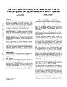
Block-Scatter Decomposition We first derive a general result for block-scatter decompositions. From this specific instances are derived. In block-scatter decompositions the data is split in a number of blocks containing consecutive data elements, each block scattered over the range of processors (fig 2a) The optimization is given in the following theorem:

Theorem 2: Block-scatter decomposition Let A' be a block-scatter-decomposition BS(b) of A with parameter b according to: A = ∆(i ← ((imin:imax)| proc(f(i)) = p) ◊ [proc(f(i)),local(f(i))]A' where proc(i) = (i div b) mod pmax and local(i) = b . (i div m.pmax))+i mod b. Let f be a monotonic increasing function, then: A = ∆(k ← (0:kp,max)) ◊ ∆(j ← (jk,p,min:jk,p,max)) ◊ [p,local(f(j))]A', where kp,max = (f(imax) div b – p) div pmax jp,k,min = max(imin, f-1(b.(p + k.pmax))) jp,k,max = min(imax,  f-1(b.(p + k.pmax) + b – 1)) ❏ Proof: We can write the equation p = (f(i) div b) mod pmax also as: p + k.pmax = t with t = f(i) div b Let the range for k be equal to 0:kmax and assume that f is a monotonic increasing function, then the value for kmax can be derived as follows: kmax = max{ k ∈ N | p + k.pmax ≤ f(imax) div b } = max{ k ∈ N | k ≤ (f(imax) div b – p) div pmax } = (f(imax) div b – p) div pmax

6

Proceedings 1991 International Conference on Parallel Processing

The range for j p,k in f(jp,k) div b = p + k.pmax can be derived as follows: b. (p + k.pmax) ≤ f(jp,k) ≤ b. (p + k.pmax) + b – 1 ⇔ f-1(b.(p+k.pmax)) ≤ jp,k ≤ f-1(b.(p+k.pmax) +b– 1) The range thus equals: jp,k,min = max(imin, f-1(b.(p + k.pmax))) jp,k,max = min(imax, f-1(b.(p + k.pmax) + b – 1))

The theorems above are also valid for monotonic decreasing functions f(i), provided that the arguments of f-1 are exchanged for tp,min and tp,max. block/scatter 0

0

1

1

2

2

3

3 0

0

1

0

1

2

3

4

5

6

7

9

10 11 12 13 14

8

1

2

2

3

(a) block 0 0

1

1 2

3

4

5

2 6

7

processor

3

8

9

10 11 12 13 14

(b) scatter

In those cases were jp,k,min > jp,k,max, there exists no integer solution for the range of jp,k.

0

1

2

3

0

1

2

3

0

1

2

❏

0

1

2

3

4

5

6

7

8

9

10 11 12 13 14

The above Theorem in fact defines a Repeated Block decomposition. However, also an alternative formulation exists: i. Repeated Scatter The formula found for the BS(b) can be rewritten by applying rules from the calculus, to obtain a form that is more favorable than the form in the previous Theorem, under the condition that b ≥ f(imax)/(2. pmax). We will refer to this form as the Repeated Scatter decomposition, as opposed to the Repeated Block decomposition presented in the above Theorem. The rewrite of A yields A = ∆(k ← ((0:kp,max)) ◊ ∆(t ← (b. p: b.p + b – 1)) ◊ ∆(j ← (jk,p,min:jk,p,max)) ◊ [p,local(f(j))]A' , where jp,k,min = max(imin, f-1(t + b. k.pmax)) jp,k,max = min(imax,  f-1(t + b. k.pmax)) = ∆(t ← (b. p: b.p+b–1)) ◊ ∆(k ← ((0:kp,max) | f-1( t + b. k.pmax) ∈ Z) ◊ [p,local(t + b. k.pmax)]A' In the following, we will explore a number of special cases of block-scatter decomposition, such as block and scatter decomposition in a general form and with a specific form of the index propagation function f. ii. Block-decomposition In the case of block-decomposition (fig2b), the general case of block-scatter decomposition reduces to BS(b), where b = f(imax)/pmax ⇔ pmax. b = f(imax). From this it follows that k p,max = (f(imax) d i v b – p ) div pmax= ((pmax. b ) div b – p) div pmax = ((pmax – p) div p max = 0, and the parameter k can be elimated altogether. The bounds for j now equal: jp,min = max(imin,f-1(b.p)) jp,max = min(imax,f-1(b.p+ b – 1))

processor

3

0

1

2

processor

(c)

Fig.2 Data Decompositions

iii. Scatter-decomposition In the case of scatter-decomposition (fig 2c), the general case of block-scatter decomposition reduces to BS(1) which yields the following simplified ranges: kp,max = (f(imax) – p) div pmax jp,k,min = max(imin, f-1(p + k.pmax)) jp,k,max = min(imax,  f-1(p + k.pmax )) The next theorem defines a more optimal version for the scatter decomposition if the function f is linear: Theorem 3: Scatter-decomposition with linear functions Consider the scatter decomposition BS(1) with function f(i) = a. i + c, a ∈ Z\{0}, c ∈ Z, then the view expression can be rewritten as: V = ∆(t ← (tp,min,tp,max)) ◊ [proc(f(genp(t)),local(f(genp(t)))]V' genp(t) = xp + (pmax/gcd(a,pmax)) . t tp,min = (imin – xp)/(pmax/gcd(a,pmax)) tp,max= (imax – xp)/(pmax/gcd(a,pmax)) where xp is a particular solution in i of the linear diophantine equation a. i – pmax. k = p – b and gcd denotes the function that yields the greatest common divisor. If no solution to the diophantine equation exists, then that particular processor is not to execute any code. ❏ Proof: The index propagation function has the form f(i) = a. i + c, a ∈ Z\{0}, c ∈ Z, and the inverse exists and equals f-1(i) = (i – c)/a. Hence by Theorem 2, we have the

7

Proceedings 1991 International Conference on Parallel Processing

following values for the bounds jp,k,min , jp,k,max and kmax: kmax = (a. imax + c – p) div pmax jp,k,min = max(imin,f-1 (p + k.pmax)) =

By choosing δp =1, i.e. p = c + gcd(a,pmax), we get xc+gcd(a, pmax) = C(a,pmax), which results from solving a. i -pmax. k - gcd(a, p max) = 0. This equation can now be used in two cases to obtain C(a,pmax) directly.

max(imin,(p + k.pmax – c)/a)) jp,k,max = min(imax,f-1 (p + k.pmax)) = min(imax,(p + k.pmax – c)/a))

Corollary 1: If pmax mod a = 0, then

Thus jp,k,min = jp,k,max iff (p + k.pmax – c)/a = i ∈ Z. This condition for k can be restated as: (p – c) = a. i – k.pmax 0 ≤ k ≤ kmax Let i = x p be a particular solution of this diophantine equation, which is obtained by the usual iterative technique of logarithmic complexity (see Section 4). Consequently, the generation function gen is given by genp(t) = x p + (pmax/gcd(a, pmax)) . t, iff (–p + c)/gcd(a, pmax)) ∈ Z. The range tp,min ≤ t ≤ tp,max can be derived from the constraint imin ≤ genp(t) ≤ imax. Substitution of genp(t) yields imin ≤ xp + (pmax/ gcd(a, pmax)).t ≤ imax and the corresponding ranges are:

❏ The solution of xp is dependent on p. This implies that we have to find x p for every value of p. This requires much work, that can not be done at compile-time, when some values, like pmax, are not known. However, as is shown in Section 4, run-time overhead can be kept low. Simplifications can be derived for a number of special cases. To this purpose, we rewrite a.i - pmax. k - p + c = 0 as (4)

with α = a/gcd(a, p max), β = p max/gcd(a, pmax), and δp = (- p+c)/gcd(a, p max). From the theory of integer equations [Gelf60], it is known that the solution of the equation is of the form: ip =δp . C(a, pmax) + β.t

genp(t) = (p-c+pmax. t)/a tp,min = (a.imin-p+c)/pmax tp,max = (a.imax-p+c)/p max ❏ Proof: If a divides pmax, then gcd(a,pmax)=a. Therefore, Eq.(4) becomes a. i - pmax. k - a = 0. It is easy to see that q=1, k=0 is a solution for this equation. Hence, C(a, pmax) =xc+a =1. From this we obtain xp =(p-c)/a, iff (pc) mod a =0. ❏ Corollary 2: If a mod pmax = 0, then genp(t) =t imin, for p=c mod pmax tp,max = imax, for p=c mod pmax

tp,min = (imin – xp)/(pmax/gcd(a,pmax)) tp,max= (imax – xp)/(pmax/gcd(a,pmax))

α.ip -β.k + δp = 0

xp = δp . C(a, pmax), iff p = c + δp . gcd(a, pmax) (6)

t= 0, ±1, ±2,.....(5)

where C(a, pmax) is a constant, solely dependent on a and pmax, hence independent on p. Both gcd(a, pmax) and C(a, pmax) can be found by using the extended Euclid's algorithm described in [Bann88]. Having found C(a, pmax), xp is simply derived as

8

tp , m i n =

❏ Proof: If p max divides a, then gcd(a,pmax)=pmax. Then Eq.(4) becomes a. i - pmax. k - pm a x = 0. From this, it follows that i=0, k=-1 is a solution. Hence, C(a,pmax) =xc+a =0. Therefore, xp =0, ∀p. However, it also holds that p = c +δp . pmax , effectively defining a single processor in the range 0≤p≤pmax-1 to be active, i.e. p=c mod pmax . ❏

Proceedings 1991 International Conference on Parallel Processing

A last observation is that in the proof of theorem 3, it has been assumed that f(i) =a.i + c. However, strictly this is not necessary, yielding the condition that the range jp,k,min : j p,k,max is not empty, iff i = f-1(p + k. pmax - c) ∈ Z. What we can do for each processor p, is check whether or not the above condition is satisfied, for k=0, 1, .., kmax, ikmax≤imax. This is of course not as optimal as the scatter decomposition of Theorem 3, since some tests may fail. For monotone non-linear functions f(i) (e.g. f(i)= i + (i div 4), f(i)= i 2 ), the method can be faster than simply enumerating on i, which would be the alternative. To see this, we rewrite the condition as f(i) = p + k. pmax c. If we enumerate on i, the sampling-rate of the lefthandside is determined by df(i)/di. If we enumerate on k, the sampling-rate is pmax , hence enumerating on k is advantageous if df(i)/di < p max, with an improvement of a factor of (pmax)/(df(i)/di). 3.3

Piece-wise monotonic functions So far, we have assumed that f(i) must be a monotonic function. However, some occurring index function in algorithms exhibit periodic behavior. Examples are index functions resulting from rotate- and perfect-shuffle type of views. Consider for instance f(i) = (i+6) mod 20, implementing a rotate operation. Clearly, functions as above are not monotonic. However, they are piece-wise monotonic. A function is piece-wise monotonic, if we can find a set of consecutive intervals [ik, ik+1 ), i min≤(ik, ik+1 )≤i max+1, ik g(imax) - g(imin). To find f-1, the modulo function has to be removed somehow. We can rewrite the function as g(i) mod z = g(i) - z . (g(i) div z)

9

Now, if there is no breakpoint in f(i), g(i) div z is a constant k and can be found by calculating k = g(imin) div z or, alternatively, k = g(imax) div z. The function f(i) then becomes g(i) - z . k +d and can be treated in the normal way. If there is a breakpoint, then it holds k=g(imin) div z and k+1=g(imax) div z. Therefore, the function is either g(i) - z . k +d or g(i) - z . (k+1) +d. The breakpoint can be found by solving ib out of g(i) mod z = 0, with imin ≤ i ≤ imax, yielding ibreak = ib . For block decomposition, the processor number where the break occurs can be found by solving f(ibreak) div c =p. At that processor the ranges must be split, according to imin ≤ i