The Law School Admission Council (LSAC) is a nonprofit corporation whose members are ... Accredited law schools outside of the United .... available online.
LSAC RESEARCH REPORT SERIES
Automatic Prediction of Item Difficulty Based on Semantic Similarity Measures
Dmitry I. Belov Lily Knezevich
Law School Admission Council Research Report 08-04 October 2008
A publication of the Law School Admission Council
The Law School Admission Council (LSAC) is a nonprofit corporation whose members are more than 200 law schools in the United States, Canada, and Australia. Headquartered in Newtown, PA, USA, the Council was founded in 1947 to facilitate the law school admission process. The Council has grown to provide numerous products and services to law schools and to more than 85,000 law school applicants each year. All law schools approved by the American Bar Association (ABA) are LSAC members. Canadian law schools recognized by a provincial or territorial law society or government agency are also members. Accredited law schools outside of the United States and Canada are eligible for membership at the discretion of the LSAC Board of Trustees. © 2009 by Law School Admission Council, Inc. All rights reserved. No part of this work, including information, data, or other portions of the work published in electronic form, may be reproduced or transmitted in any form or by any means, electronic or mechanical, including photocopying and recording, or by any information storage and retrieval system, without permission of the publisher. For information, write: Communications, Law School Admission Council, 662 Penn Street, Box 40, Newtown, PA 18940-0040. This study is published and distributed by LSAC. The opinions and conclusions contained in this report are those of the author(s) and do not necessarily reflect the position or policy of LSAC.
i
Table of Contents Executive Summary . . . . . . . . . . . . . . . . . . . . . . . . . . . . . . . . . . . . . . . . . . . . . . . . . . . . . . . . . . . . . . . . . . . . . . . . . . . . . . . . . . . . . . . 1 Introduction. . . . . . . . . . . . . . . . . . . . . . . . . . . . . . . . . . . . . . . . . . . . . . . . . . . . . . . . . . . . . . . . . . . . . . . . . . . . . . . . . . . . . . . . . . . . . . . 1 WordNet . . . . . . . . . . . . . . . . . . . . . . . . . . . . . . . . . . . . . . . . . . . . . . . . . . . . . . . . . . . . . . . . . . . . . . . . . . . . . . . . . . . . . . . . . . . . . . . . . 1 An Algorithm to Compute a Semantic Similarity Matrix of Two Texts . . . . . . . . . . . . . . . . . . . . . . . . . . . . . . . . . . . . . . . . . . 3 Semantic Similarity Measures . . . . . . . . . . . . . . . . . . . . . . . . . . . . . . . . . . . . . . . . . . . . . . . . . . . . . . . . . . . . . . . . . . . . . . . . . . . . . . 4 Graph Theory Approach. . . . . . . . . . . . . . . . . . . . . . . . . . . . . . . . . . . . . . . . . . . . . . . . . . . . . . . . . . . . . . . . . . . . . . . . . . . . . . . . 4 Geometric Approach . . . . . . . . . . . . . . . . . . . . . . . . . . . . . . . . . . . . . . . . . . . . . . . . . . . . . . . . . . . . . . . . . . . . . . . . . . . . . . . . . . 4 Algebraic Approach . . . . . . . . . . . . . . . . . . . . . . . . . . . . . . . . . . . . . . . . . . . . . . . . . . . . . . . . . . . . . . . . . . . . . . . . . . . . . . . . . . . 4 Experiments with LSAT Items . . . . . . . . . . . . . . . . . . . . . . . . . . . . . . . . . . . . . . . . . . . . . . . . . . . . . . . . . . . . . . . . . . . . . . . . . . . . . . 5 Description of the Studied Item Type . . . . . . . . . . . . . . . . . . . . . . . . . . . . . . . . . . . . . . . . . . . . . . . . . . . . . . . . . . . . . . . . . . . . . 5 Decision Tree . . . . . . . . . . . . . . . . . . . . . . . . . . . . . . . . . . . . . . . . . . . . . . . . . . . . . . . . . . . . . . . . . . . . . . . . . . . . . . . . . . . . . . . . 5 Feature Space Augmentation. . . . . . . . . . . . . . . . . . . . . . . . . . . . . . . . . . . . . . . . . . . . . . . . . . . . . . . . . . . . . . . . . . . . . . . . . . . . 5 Results . . . . . . . . . . . . . . . . . . . . . . . . . . . . . . . . . . . . . . . . . . . . . . . . . . . . . . . . . . . . . . . . . . . . . . . . . . . . . . . . . . . . . . . . . . . . . . . 6 Discussion . . . . . . . . . . . . . . . . . . . . . . . . . . . . . . . . . . . . . . . . . . . . . . . . . . . . . . . . . . . . . . . . . . . . . . . . . . . . . . . . . . . . . . . . . . . . . . . . 6 References . . . . . . . . . . . . . . . . . . . . . . . . . . . . . . . . . . . . . . . . . . . . . . . . . . . . . . . . . . . . . . . . . . . . . . . . . . . . . . . . . . . . . . . . . . . . . . . 6 Acknowledgments . . . . . . . . . . . . . . . . . . . . . . . . . . . . . . . . . . . . . . . . . . . . . . . . . . . . . . . . . . . . . . . . . . . . . . . . . . . . . . . . . . . . . . . . . 7
1
Executive Summary Item difficulty modeling (IDM) assimilates various techniques from data mining, pattern recognition, and natural language processing. The primary task of IDM is to estimate the statistical properties of a test question (item), such as difficulty, based on features extracted directly from the item. An example of such a feature might be the number of rarely used words in the passage and in the correct/incorrect answer choices in a multiple-choice item. The corresponding feature space can be partitioned using a decision tree analysis. In this way, the impact of a feature on item difficulty and other statistical characteristics can be validated. IDM can be applied to enhance many routine psychometric analyses. Additionally, IDM can help testing organizations manage the pretesting of new items more efficiently, since estimates of item difficulty can be available before pretest statistics are obtained. This study was motivated by the results of research on item pool analysis and design. It was shown that items with certain content and statistical characteristics could dramatically improve the ability of an item pool to support the assembly of test forms. Although item writers are able to control the content characteristics of items, item difficulty is not so easily controlled. Therefore, there is a practical demand for automated tools to predict item difficulty. This report introduces new automated features for predicting item difficulty based on WordNet—a lexical database available online. Methods for computing a semantic similarity measure between two texts and a self-similarity measure of a text are developed. Each method is based on certain characteristics of the semantic similarity matrix of two texts, where each element of the matrix measures the semantic similarity of two corresponding words. Based on these measures, a decision tree for predicting item difficulty is constructed and validated. The results of experiments with reading comprehension items show that the new features are useful for predicting item difficulty. In particular, they predicted correctly in 83–86% of cases, which was 11–14% higher than the prediction based on the Breland Word Frequency index.
Introduction Item difficulty modeling (IDM) attempts to estimate an item’s statistical properties, such as difficulty or discrimination, based on features extracted directly from the item. An example of such a feature is the minimum value of the Breland Word Frequency (BWF) index (Breland, Jones, & Jenkins, 1994) in an item’s passage, key, and distractors (Sheehan & Mislevy, 2001). IDM can be applied for item parameter estimating (Mislevy, 1988), equating (Mislevy, Sheehan, & Wingersky, 1993), and creating an evidence-centered examinee model (Mislevy, Almond, Yan, & Steinberg, 1999; Sheehan, Kostin, & Persky, 2006). Huff (2006) provides a thorough review of IDM and its applications. This particular work was motivated by the results of research on item pool analysis and design (Belov & Armstrong, 2005, 2008). It was shown that the addition of items with certain content and statistical characteristics could dramatically improve pool usability. Belov and Armstrong (2005) considered a depleted pool of 987 items from which no section for the Law School Admission Test (LSAT) could be assembled. After a single item was added to the pool, a new section for the LSAT could be assembled. Although item writers are able to control the content characteristics of items, item difficulty is not so easily controlled. Therefore, there is a practical demand for automated tools to predict item difficulty. Recent studies have explored new sources of item features for application in IDM (Gorin, 2006; Sheehan et al., 2006). For example, Sheehan et al. (2006) used semantic relatedness between texts by applying a latent semantic analysis by Landauer and Dumais (1997). This analysis is based on characteristics of a large matrix of word-by-document frequencies and, therefore, is sensitive to specific observed data. This report explores an approach to measuring semantic similarity based on WordNet (Fellbaum, 1998), which is independent from the observed data (Resnik, 1998). The first section briefly describes the WordNet lexical database and its application to measure semantic similarity between two words. The second section describes an algorithm to compute a matrix of semantic similarity between two texts. The third section introduces three approaches to computing semantic similarity between two texts and self-similarity of a text. The fourth section presents the results of experiments with LSAT items. A discussion is presented in the final section of the report.
WordNet WordNet (Fellbaum, 1998) is a semantic dictionary designed as a graph. To our knowledge, no studies have applied WordNet to predict item difficulty.
2 The smallest unit in WordNet is a synset, which represents a specific meaning of a word. It includes the word, its explanation, and its synonyms. Synsets are connected to one another through explicit semantic relationships, forming a semantic graph. In WordNet, given a part of speech (noun, verb, adjective, adverb) and semantic relationship (hypernyms for nouns and verbs; synonyms for adjectives and adverbs), a word can have multiple synsets (Fellbaum, 1998). Figure 1 shows paths to the corresponding synsets for two words: psychometrics and psychophysics.
(a)
(b) FIGURE 1. Semantic paths for two words in WordNet: (a) psychometrics; (b) psychophysics
3
A semantic similarity between two synsets can be computed from the distance between corresponding nodes in the semantic graph. The shorter the distance from one node to another, the more similar they are (Resnik, 1998). The distance ( s, t ) is the number of nodes between (and including) node s and node t. Figure 2 shows a fragment of a subgraph formed by two paths from Figure 1.
…
Science, scientific discipline
Psychology, psychological science
Experimental psychology, psychonomics
Psychometrics
Psychophysics FIGURE 2. An example showing the shortest distance between psychometrics and psychophysics
We use the following formula to compute semantic similarity between two words:
ls ,lt ( s, t )
1 , ( s, t )
(1)
where ls is the selected path of s and lt is the selected path of t. The similarity is zero if the paths have no common nodes or no path exists. For example, if s = psychometrics and t = psychophysics, then the similarity in (1) is 0.25, since four nodes are counted, beginning with psychometrics and terminating with psychophysics (see Figure 2). Other methods of computing semantic similarity between two words can be found in http://marimba.d.umn.edu/similarity/measures.html.
An Algorithm to Compute a Semantic Similarity Matrix of Two Texts Given two texts (both can be the same), the following is a simplified version of an algorithm by Simpson and Dao (2005). Matrix Algorithm Step 1 (Tokenization):
Each text is transformed into a vector of words, where frequently occurring or insignificant words are removed. For example, consider these two texts: Text 1 = “Correlation does not necessarily imply causation.” Text 2 = “Causation and correlation are easily confused terms.” The result of Step 1 will be two vectors: x ( x1 , x2 ,..., xm ) = (correlation, necessarily, imply, causation) y ( y1 , y2 ,..., yn ) = (causation, correlation, easily, confused, terms)
4
Step 2 (Computing a semantic similarity matrix):
Compute m n matrix R such that rij max lx ,l y ( xi , y j ) [see formula (1)] is the maximal semantic l xi ,l y j
i
j
similarity between words xi and y j , where i 1, 2,..., m , j 1, 2,..., n , and variables lxi , l y j loop through all semantic paths of xi , y j . To construct a correct semantic path, each word is transformed by the WordNet morphology function to its base form; for the above example, the word terms will be transformed to term. For the above example we have the following matrix: 1 0.09 0 0 R 0 0 0.09 1
0.13 0 0 0.2 0 0 0 0.08 0 0
0 0
Semantic Similarity Measures This section introduces several methods for computing semantic similarity between two texts and self-similarity of a text. Each method is based on one of the following three approaches to the semantic similarity matrix: the graph theory approach, the geometric approach, and the algebraic approach. Graph Theory Approach
The graph theory approach, introduced by Simpson and Dao (2005), is based on an interpretation of matrix R as the adjacency matrix of a bipartite weighted graph. The maximum weighted matching will provide an estimate of semantic similarity between two texts, and it can be found in polynomial time by the Hungarian method (Papadimitriou & Steiglitz, 1982). In this report we use the following normalized approximation: m
(x, y )
i 1
n
n
max rij j 1
j 1
mn
m
max rij i 1
,
where 0 (x, y ) 1 . We apply (x, y ) to compute the semantic self-similarity measure of a text and denote it as (x). When x y, matrix R is square and symmetric with diagonal elements equal to 1. This will produce a value for (x) 1 . To avoid this trivial solution, we assign zero to all diagonal elements of matrix R. The major disadvantage of the graph theory approach is that not all of the elements of matrix R contribute to the measure. The next two new approaches will address this disadvantage. Geometric Approach
The geometric approach interprets rows of matrix R as interior points of the hypercube {z n | 0 zi 1} in an n -dimensional vector space n . The closer these points are to the vertex (1,1,....,1), the greater the corresponding similarity. Thus we can apply the following steps: (a) compute the mean vector of the rows of R, (b) compute the length of the mean vector, and (c) divide the length by n . We denote the corresponding semantic similarity between two texts as (x, y ) and the semantic self-similarity of a text as (x). Both measures fall within the [0,1] range. Algebraic Approach The extreme case of matrix R is when all of its elements equal 1. Therefore, the greater the largest eigenvalue of the square symmetric matrix R, the higher the semantic self-similarity of the corresponding text. In order to apply the algebraic approach to compute the semantic similarity between two texts, we use the largest singular value of matrix R.
5 To normalize, we divide by m, where m n. We denote the corresponding semantic similarity between two texts as (x, y ) and the semantic self-similarity of a text as (x). Both measures fall within the [0,1] range.
Experiments with LSAT Items This section presents the results of experiments on predicting item difficulty for LSAT items. First, we describe the item type chosen for the study. Next, we discuss the major steps of constructing a decision tree to predict item difficulty based on the semantic similarity measures from the previous section. Finally, we present the results of the validation of different decision trees. Description of the Studied Item Type The LSAT consists of four equally timed, scored sections. One of these sections is devoted to the Reading Comprehension (RC) item type. The RC item type is set-based. Each RC section consists of four RC sets. For each set, the test taker is asked to read a passage of approximately 450 words and answer between five and eight questions about the passage. The passages contain sophisticated argumentation or other complex relationships among ideas so as to exhibit a unified main point or central idea. The test taker is expected to understand that central idea or point of view on first reading of the passage. Virtually all RC sets begin with an item that asks the test taker to identify the main point or central idea. These items fall into the “Main Point” RC (MPRC) subtype. The MPRC subtype will ask the test taker to identify the statement that best expresses the central idea, main idea, or main point that the passage as a whole is designed to convey. The item stem, or the explicit question asked, asks the test taker to identify the main point of the passage if the overall structure of the passage is argumentative. If the passage is not so clearly structured as an argument, the item stem will ask the test taker to identify the main idea of the passage. Decision Tree Currently, the most popular approach for predicting item difficulty is to construct a regression tree from items, each with known difficulty and a given set of features (Huff, 2006; Sheehan, Kostin, & Futagi, 2007; Sheehan et al., 2006). Then the features of an item with unknown difficulty are used to branch through the nodes of the tree until the corresponding terminal node is reached. Finally, the expectation of the difficulty among items from the terminal node (or least-squares solution if there are enough items) is used as a prediction. Based on semantic similarity measures, a regression tree (Breiman, Friedman, Olshen, & Stone, 1984) for predicting item difficulty can be constructed. The following algorithm describes the major steps to constructing the regression tree: Tree Algorithm Step 1 (Forming a feature space): Selected measures, including , , defined above, are computed for each item to form a feature space. Step 2 (Building a decision tree): Binary splits are applied to the feature space to construct a decision tree. Each split minimizes the variance of the p+ at each corresponding node, where p+ denotes the item proportion correct statistic. At each node, the minimum number of items was 1 and the minimal improvement for each candidate split was 0.05. Feature Space Augmentation In order to take into account linear combinations of various features, we augment the feature space. First, we transform the coordinate system, such that it is shifted to the mean vector of the feature space. Second, we augment each vector of the feature space by its projection to the eigenvectors of the covariance matrix (Searle, 1982) of the feature space. A more general approach would be to use linear combination splits (Breiman et al., 1984) on Step 2 of the Tree Algorithm. Alternatively, Sheehan et al. (2007) applied factor analysis to reduce a large number of features to a smaller number of dimension scores and then constructed a regression tree from the dimension scores.
6
Results All algorithms were implemented in C++ and C# for Windows using WordNet, WordNet.Net (Crowe and Simpson, 2005), and IMSL libraries. The results of the study follow. A decision tree was constructed by applying the Tree Algorithm to 64 disclosed MPRC items. The following crossvalidation procedure was used: (1) an item is removed from the set of 64 items; (2) a tree is constructed for the remaining 63 items; (3) using the tree, a prediction is made for the removed item; (4) the predicted p+ is compared with the true p+ (if the distance between the predicted and true p+ was less than or equal to 0.2, the item was said to be correctly classified); (5) the item is returned back to the set; (6) steps 1–5 are repeated for the next item until all 64 items are processed. Table 1 demonstrates the results of the above validation procedure applied to four different feature spaces: BWF space, space, space, and space. The BWF space has three dimensions and includes the minimum value of the BWF index in the passage, key, and distractors. The space has three dimensions and includes semantic similarity between: passage and key; passage and distractors; and key and distractors. The space has three dimensions and includes semantic similarity between: passage and key; passage and distractors; and key and distractors. The space has seven dimensions and includes semantic self-similarity of passage, passage+[option A], passage+[option B], passage+[option C], passage+[option D], passage+[option E], passage+[option A]+ [option B]+ [option C]+ [option D]+ [option E]. One can see that the semantic similarity measures predicted better than the BWF index (see Table 1). The best results were achieved by applying semantic similarity . TABLE 1 Results of cross-validation procedure applied to four different feature spaces Number of Feature Space # Feature Space Dimensions True Positives 1 BWF space 3 72% 2 space 3 78% 3 space 3 86% 4 space 7 83%
Bias −0.028 0.004 0.003 −0.005
MSE 0.043 0.030 0.027 0.028
Discussion Our approach to item difficulty modeling is fully automatic: It utilizes new methods for computing semantic similarity measures and draws from the publicly available WordNet. Preliminary results suggest that semantic similarity between two texts [ (x, y ), (x, y ), (x, y )] and semantic self-similarity of a text [ (x), (x), (x)] are useful for predicting item difficulty of MPRC items since they predicted about 6–14% better than the BWF index (see Table 1). Semantic similarity measures , demonstrated better prediction rates than (see Table 1). The Matrix Algorithm should be refined because at Step 2, for each pair of words, it maximizes measure (1) over all possible parts of speech and all possible senses. The extension should include part-of-speech tagging and word-sense disambiguation. A simpler alternative would be to compute separate semantic similarity matrices for nouns, verbs, adjectives, and adverbs, which would provide more refined measures of semantic similarity. The standard indicator of the vocabulary difficulty of a text is a minimum value of the BWF index. However, alternative methods can be applied. For example, we can apply the polysemy count of a word from WordNet or employ an Internet search engine (e.g., www.google.com, www.ask.com) under various filters. We wrote a simple code in C++ that uses standard HTTP to automatically acquire the number of search hits for a given word under different filters. This code was used to construct an Internet word frequency (IWF) index similar to the BWF index. IDM provides a methodology for improving many aspects of educational assessment: item parameter estimation (Mislevy, 1988), test equating (Mislevy et al., 1993), evidence-centered design (Mislevy et al., 1999; Sheehan et al., 2006), and item pool maintenance. Additionally, IDM can help testing organizations manage the pretesting of new items more efficiently, since estimates of item difficulty are available before pretest statistics are obtained.
References Belov, D. I., & Armstrong, R. D. (2005). Monte Carlo test assembly for item pool analysis and extension. Applied Psychological Measurement, 29, 239–261. Belov, D. I., & Armstrong, R. D. (2008). A Monte Carlo approach to the design, assembly and evaluation of multi-stage adaptive tests. Applied Psychological Measurement, 32, 119–137. Breiman, L., Friedman, J. H., Olshen, R., & Stone, C. J. (1984). Classification and regression trees. Belmont, CA: Wadsworth International Group.
7
Breland, H. M., Jones, R. J., & Jenkins, L. (1994). The College Board Vocabulary Study. New York, NY: College Entrance Examination Board. Crowe, M., & Simpson, T. (2005). WordNet.Net Library. http://opensource.ebswift.com/WordNet.Net/Default.aspx Fellbaum, C. (Ed.). (1998). WordNet: An electronic lexical database. Cambridge, MA: MIT Press. Gorin, J. S. (2006, April). Using alternative data sources to inform item difficulty modeling. Paper presented at the Annual Meeting of the National Council on Measurement in Education, San Francisco, CA. Huff, K. (2006, April). Using item difficulty modeling to inform descriptive score reports. Paper presented at the Annual Meeting of the National Council on Measurement in Education, San Francisco, CA. Landauer, T. K., & Dumais S. T. (1997). A solution to Plato’s problem: The latent semantic analysis theory of acquisition, induction, and representation of knowledge. Psychological Review, 104, 211–240. Mislevy, R. J. (1988). Exploiting auxiliary information about items in the estimation of Rasch item difficulty parameters. Applied Psychological Measurement, 12, 281–296. Mislevy, R. J., Almond, R. G., Yan, D., & Steinberg, L. S. (1999). Bayes nets in educational assessment: Where the numbers come from. In K. B. Laskey & H. Prade (Eds.), Proceedings of the Fifteenth Conference on Uncertainty in Artificial Intelligence (pp. 437–446). San Francisco: Morgan Kaufmann. Mislevy, R. J., Sheehan, K. M., & Wingersky, M. S. (1993). How to equate tests with little or no data. Journal of Educational Measurement, 30, 55–78. Papadimitriou, C. H., & Steiglitz, K. (1982). Combinatorial optimization: Algorithms and complexity. Englewood Cliffs, NJ: Prentice-Hall. Resnik, P. (1998). WordNet and class-based probabilities. In C. Fellbaum (Ed.), WordNet: An electronic lexical database (pp. 239–263). Cambridge, MA: MIT Press. Searle, S. R. (1982). Matrix algebra useful for statistics. New York: John Wiley & Sons, Inc. Sheehan, K. M., Kostin, I., & Futagi, Y. (2007, March). Predicting text difficulty via corpus-based dimensionality reduction and tree-based regression. Presented at the Turnball Hall Seminar Series. Princeton, NJ: Educational Testing Service. Sheehan, K. M., Kostin, I., & Persky, H. (2006, April). Predicting item difficulty as a function of inferential processing requirements: An examination of the reading skills underlying performance on the NAEP grade 8 reading assessment. Paper presented at the Annual Meeting of the National Council on Measurement in Education, San Francisco, CA. Sheehan, K. M., & Mislevy, R. J. (2001). An inquiry into the nature of the sentence-completion task: Implications for item generation. Princeton, NJ: Educational Testing Service. Simpson, T., & Dao, T. (2005). WordNet-Based Semantic Similarity Measurement. http://www.codeproject.com/KB/string/semanticsimilaritywordnet.aspx
Acknowledgments We are grateful to Susan Dalessandro and Jennifer Lawlor for their assistance in preparation of the data for this project. Also we would like to thank Ronald D. Armstrong, Lynda M. Reese, and Alexander Weissman for their valuable suggestions and comments on previous versions of the manuscript.