ABSTRACT. We propose an algorithm to detect salient regions for JPEG dis- torted images for two tasks: quality assessment and free viewing. The algorithm ...
2011 Third International Workshop on Quality of Multimedia Experience
AUTOMATIC PREDICTION OF SALIENCY ON JPEG DISTORTED IMAGES Anish Mittal, Anush K. Moorthy and Alan C. Bovik
Lawrence K. Cormack
Department of Electrical and Computer Engineering University of Texas at Austin
Department of Psychology University of Texas at Austin
ABSTRACT We propose an algorithm to detect salient regions for JPEG distorted images for two tasks: quality assessment and free viewing. The algorithm extracts low-level features such as contrast, luminance, quality and so on and uses a machine-learning framework to predict salient regions in JPEG distorted images. We demonstrate that the automatically predicted regions-of-interest highly correlate with those from (human) ground truth saliency maps. Further, we evaluate the relevance of extracted low-level features for saliency prediction and analyze how incorporation of quality as a feature improves prediction performance as a function of the distortion severity. Applications of such a saliency prediction framework include developing novel pooling strategies for image quality assessment. Index Terms— Bottom up, Eye movements, Image compression, Visual attention, Saliency Prediction, Quality Assessment, Task-dependence 1. INTRODUCTION Humans are constantly bombarded with a slew of visual information which is rapidly processed in order to make inferences about the environment as well as to perform quotidian tasks such as navigation, interaction with objects and so on. While humans possess a wide field of view, visual information is made available to the human visual system (HVS) with varying amounts of acuity – visual acuity is highest at the fovea, and lowest at the periphery. In order to reproduce the entire field of view at an uniform resolution, the HVS utilizes a series of fixations which gather maximum information from a scene, linked together by rapid ballistic eye movements known as saccades, which gather little-to-no information [1]. Seemingly, such a multi-resolution system with a dynamic system of actively scanning the scene results in efficient representation of visual information. Given the active scanning apparatus of the HVS, one would hypothesize that certain regions in a scene have greater relevance for the human observer and hence act as attractors of visual attention. Researchers have classified gaze selection mechanisms into those that are based on low-level features such as local luminance, contrast and so on – referred to as bottom-up cues – and those that are based on higher-level abstractions of the scene such as faces, spatial relationships of objects etc. – referred to as top-down cues [1]. Researchers have suggested that initial regions of attention are driven by low-level cues, while semantic information starts to play a greater role over time [2]. While higher-level abstractions of the scene are definitely of relevance, the sheer volume of data that needs to be processed in order to make such a high-level inference suggests that bottom-up cues may contribute significantly in attracting visual attention, and hence we focus our attention on modeling such bottomup cues [1, 3, 4, 5].
978-1-4577-1334-7/11/$26.00 ©2011 IEEE
195
One such low-level cue that possibly attracts visual attention is the quality of the image. Researchers have observed that presence of distortion in a scene draws visual attention [6, 7, 8, 9, 10, 11]. Miyala et al. conducted a subjective study to track gaze behavior of human observers while viewing distorted images [7]. Blur, noise and color shifts were used to degrade the images. They found that these distortions had no affect on viewing strategies. Ninassi et al. [6] introduced local distortions like JPEG2000 and JPEG compression in images and concluded that for these distortions viewing strategies were indeed affected by the presence of distortion, however, effects of distortion severity was not taken in to consideration in the study. Vu et al. performed a more comprehensive task dependent evaluation of how different distortions (blur, noise, JPEG and JPEG2000 compression) and different levels distortion severities modify viewing strategies [8]. As Yarbus demonstrated in his pioneering work, the task performed defines visual attention, and a change in the task results in a different viewing strategy [1]. Indeed, researchers have proposed different models to predict regions of visual attention conditioned on the task [12]. In [8], two different tasks were considered – free viewing and quality assessment. The authors concluded that viewing strategies remain similar for both tasks in case of global distortions such as blur and noise; however JPEG and JPEG2000 creates marked differences in viewing patterns across tasks as well as across distortion severities. Earlier, we [10, 11] analyzed various low level features at point of gaze for compressed videos at different distortion severities and for two different tasks – quality assessment task and summarization. We observed that there exist statistically significant differences between low-level features at points-of-gaze across tasks, as well as across distortion severities. Having empirically observed significant differences in viewing strategies in the presence of distortion, an obvious route to follow is to try and model visual attention strategies of human observers, as a function of the task as well as the distortion severity. Our contribution is an algorithm which predicts visual attention in static scenes, subject to JPEG compression, as a function of the task – quality assessment vs. free-viewing. Our approach to such automatic prediction of visual attention in distorted images consists of extracting low-level attractors of attention from the scene, ‘learning’ the relative importance of each of these attractors and then using this trained model to predict attention in unseen images. Our work is similar in nature to those in [3, 4, 5], which predict saliency and fixations in natural images, however, our algorithm is geared towards such prediction for distorted images, while those in [3, 4, 5] predict visual attention in natural, undistorted, pristine images. Such automatic prediction of visual attention in distorted images has many applications, including development of novel pooling strategies for image quality assessment (IQA). In this paper, we motivate and describe the various low-level features that we extract from the scene and our training-based model for prediction of visual attention. We then undertake a thorough evaluation of the algorithm and compare our au-
2011 Third International Workshop on Quality of Multimedia Experience
tomatic prediction results with those from human observers using a variety of performance measures and demonstrate that our approach is capable of predicting visual attention with high correlation with human perception. 2. AUTOMATIC PREDICTION OF VISUAL ATTENTION In this section, we first describe the database that we are going to use in order to evaluate our algorithm. We then describe the various low-level features that we extract from the scene and detail how these features are combined in order to create an algorithm which predicts attention in distorted images. 2.1. Database Description The database that we use in order to test our approach is the Tu Delft database, proposed by researchers in [13]. In [13], the researchers conducted a human study, where subjects viewed images compressed by JPEG compression with 4 different compression (quality) levels, while their eye-movement locations were recorded using an IView X system eye tracker [14] with sampling rate 50 Hz. The stimuli were displayed on a 17-inch CRT monitor at a resolution of 1024 × 768 pixels and viewed at a distance of 60 cm from the screen. Apart from varying distortion severity, the study also consisted of two different tasks – quality assessment and free-viewing. In the former, participants were required to examine the images and rate them based on their quality; participants were allowed to examine the image until they decided on the quality score. In the latter, participants were asked to view the images in a casual manner as if they were viewing a photo album and each image was displayed for 8 seconds on the screen. The points of gaze from subjects were then post-processed to produce saliency maps, which are representative of regions of visual interest. The Tu Delft database consists of 40 reference images, 160 distorted images and associated saliency maps for each of these distorted images, where the images are of resolution 600 × 600 pixels and is available for download at [15]. Having described the database on which we perform our experiments, we now describe the low-level features that we extract from these static images and the motivation for their choice. 2.2. Feature Extraction We first decompose the image using the steerable pyramid transformation [16], an over complete wavelet basis that has been successfully used in the past for a variety of applications, including texture analysis [17], quality assessment [18] and so on. Such a wavelet decomposition over multiple scales and orientations seeks is inspired from the scale-space orientation decomposition that is hypothesized to occur in area V1 of the primary visual cortex [19]. In our implementation, we first transform the color image into the perceptually uniform, color opponent CIE-Lab color space [20] and then decompose each of the L, a and b planes over 3 scales and 4 orientations. Increasing the number of scales or orientations did not lead to any tangible performance improvement. The absolute value of the wavelet coefficient is normalized by the mean of the absolute value in each sub band. Our first feature at each pixel location is the local average value of this normalized magnitude of wavelet coefficient, where the local average is computed by centering a Gaussian filter the size of 1 degree of visual angle (41 × 41 for our viewing distance) at that pixel. We sample the Gaussian out to 3 standard deviations. Each wavelet sub band is interpolated back to the image scale using bi cubic interpolation, and
196
hence at each pixel location, we have a total of 3 (scales) × 3 (orientations) × 3 (color planes) = 36 features corresponding to band-pass contrast. Selection of different interpolation schemes did not affect the performance. Further, at each pixel, we also compute the local average luminance and chrominance value from the 3 color planes. Again, the local average luminance/chrominance is computed using the above described Gaussian filter, leading to 3 additional features at each pixel corresponding to the luminance in that region. These bandpass and luminance features (total of 39) are collectively labeled as bandpass contrast and luminance (BPCL) features. Since our goal is to predict visual attention in distorted images, and our hypothesis is that degradations in visual quality are lowlevel attractors of attention, we also include quality at each pixel in our list of features. In order to automatically estimate quality, we use the multi-scale structural similarity (MS-SSIM) index [21]. In our implementation, the five scales of quality produced by the MSSSIM index are not combined into one quality score for the image as in [21], since our goal is to provide a quality estimate at each pixel location. Instead, we use bicubic interpolation to resample the lower scales back to the image scale, so that at each pixel location we have a 5-dimensional quality vector, corresponding to the 5 different scales. Again, the feature is the average local quality value from each of these scales, computed using the described Gaussian filter, leading to a total of 5 quality features (Q) at each pixel. Apart from low-level BPCL and Q features, we also compute the distance of each pixel location to the center, in order to account for the natural human bias towards the center when viewing a scene [5]. This distance-to-center (D) forms our last feature. 2.3. Training the model Once these features have been extracted, we use the saliency maps from the database described above in order to learn a relationship between the features and the saliency. For this, we divide the database into two sets, one for training and the other for testing, such that there is no content overlap between the two sets. 80% of the distorted images are used for training and the remaining 20% are used for testing. Such a train-test methodology is performed for each of the two tasks separately, i.e., a model is trained for the free-viewing task and then tested on the free-viewing test images and similarly for quality assessment. We also perform across-task evaluations, which we explain in later sections. Further, such an evaluation is performed over multiple (50) such randomly chosen train-test combinations, in order to demonstrate the robustness of the model to various train-test combinations. We train a classifier to differentiate between salient and nonsalient regions. Salient regions are easily obtained from the saliency maps. For this, the top x% salient locations of the human ground truth saliency map are chosen and n salient locations are drawn uniformly at random from this set. In our implementation, x corresponds to 0.5σ, where σ is the standard deviation of the saliency map. Since each image has a different distribution of salient regions (eg., a human rowing a boat vs. a crowded street scene), such use of the standard deviation will capture this diversity. In order to obtain non-salient locations, we utilize the strategy proposed in [3], where random locations are not chosen uniformly at random, but for each image the set of non-salient locations are computed by applying the saliency map of another randomly chosen image (different content) from the distorted images in the training set. This ensures that while the non-salient locations are random, the underlying search strategy that generated these regions of interest have close correspondence with human search mechanisms. We also
2011 Third International Workshop on Quality of Multimedia Experience Reference Test Images
Reference Training Images
Quality Features
Distorted Test Images
Distorted Training Images
Band pass luminance and contrast features
Distance from center features
Training Model
Feature Weights
test Model
Saliency Map
Fig. 1. Block diagram of saliency selection model. The solid arrows walk through block diagram of training phase where quality, band pass luminance & contrast and distance from center features are computed for every training image and hence used for learning the feature weights of the linear SVM classifier. The dotted lines depict testing phase where same features are computed for a test image and saliency is computed by using feature weights from trained classifier.
Fig. 2. Figure showing samples of JPEG distorted images from the Tu Delft database on the left, ground truth saliency obtained in the middle and predicted saliency maps on the right from the free viewing task.
ensure that the non-salient locations at least 1 degree of visual angle away from the salient locations in the image, in order to minimize overlap between them. For each image, n such non-salient locations are selected. Through the rest of this paper, n is set to 12, since varying the number of salient/non-salient regions between 8 − 24 did not affect performance much. Feature vectors are extracted at each of the salient and nonsalient locations as described above, and these features are used to train a classifier that once trained is capable of classifying an image patch into a salient region vs. a non-salient one. Here, we use the liblinear implementation of a support vector machine (SVM) with a linear kernel [22]. Linear kernels have been shown to perform as well as multiple kernel learning or radial bias kernels for fixation selection [5], and training is much faster as well. Instead of using the trained classifier as a simple binary classifier, in our implementation, during the testing phase, we use the value of wT x + w0 , which indicates the degree of saliency at each pixel, where w corresponds to the weights learned from the training phase for each feature and w0 corresponds to the offset. The entire model is summarized by a block diagram in Fig. 1. As an example, figures 2 and 3 show a set of sample JPEG distorted images from the Tu Delft database, ground truth saliency maps and predicted saliency maps for each of the two tasks – free viewing and quality assessment – respectively. 3. PERFORMANCE EVALUATION Having described the features extracted and the training procedure, in this section we evaluate our model using two measures of performance: (1) Location percentage thresholding based Receiver Operating Characteristic (LPT-ROC) and (2) Saliency based thresholding Receiver Operating Characteristic (SBT-ROC).
197
Fig. 3. Figure showing samples of JPEG distorted images from the Tu Delft database on the left, ground truth saliency obtained in the middle and predicted saliency maps on the right from the quality assessment task.
2011 Third International Workshop on Quality of Multimedia Experience 1
Location percentage thresholding based Receiver Operating Characteristic (LPT-ROC): For every test image, pixel values of the predicted and ground truth saliency maps (values between 0 and 1) are sorted in the descending order of saliency, and recall and precision are computed as described in [5]. Specifically, we compute: CumF (i) =
0.8
0.7
0.6 Precision
i X
0.9
F (k) i = 1, ....N
(1)
0.5
0.4
k=1 0.3
CumN F (i) =
i X
(1 − F (k)) i = 1, ....N
0.2
(2)
CumF (i) P recision(i) = PN k=1 F (k) CumN F (i) Recall(i) = PN k=1 (1 − F (k))
0
(3) (4)
0.2
0.3
0.4
0.5 Recall
0.6
0.7
k=1
k=1 P recision(k) t = 1, ....T N
0.9
1
0.8
0.7
0.6
0.5
0.4
0.3
0.2
PN
0.8
0.9
Precision
PN
HumanPerformance BPCL features BPCL + Q features BPCL +Q +D features Chance
0.1
(6) 0
Finally, the AAUC averaged across trials is computed as:
0
0.1
0.2
0.3
0.4
0.5 Recall
0.6
0.7
0.8
0.9
1
(b)
PT
AAU C(k) (7) T where N is the total number of pixels in the test image, F represents the saliency map and L denotes the number of test images in a single trial and T denotes the number of trials. The final performance measure is then the ratio of the TAAUC between the predicted map and ground truth saliency map. T AAU C =
0.1
(a)
P recision(k) l = 1, ....L (5) N The average Area under ROC curve (AAUC) across test images in a single trial is then computed as: AAU C(t) =
0
1
Since each test trial consists of multiple such test images, we compute the area under ROC curve (AUC) for each image in the test set as: AU C(l) =
HumanPerformance BPCL features BPCL + Q features BPCL +Q +D features Chance
0.1
k=1
k=1
Fig. 4. Figure shows the average LPT-ROC curve for (a) free viewing and (b) quality assessment task across 50 trials using different set of features. BPCL denotes band pass contrast and luminance, Q denotes quality and D denotes distance from center.
3.1. Effect of Feature Type Saliency based thresholding Receiver Operating Characteristic (SBT-ROC): Since we only have access to the saliency map, we first binarize this map into salient and non-salient regions. As before, this is done by thresholding the saliency map at 0.5σ, where σ is the standard deviation of the saliency map. Once such a binary ground-truth is obtained, the SBT-ROC can be computed by the traditional thresholding of the predicted saliency maps as a function of saliency [23]. The ROC curve is sampled uniformly at 20 such saliency thresholds and for each such threshold, a point on the ROC is obtained. The performance measure is then the traditional area under the ROC curve (AUC). We note that both ROC measures are complementary to each other. The first measure compares the overall saliency distribution of the predicted and ground truth maps while the second measure compares just the top salient locations between the two maps. Having described our performance measures, we now perform a series of experiments in order to evaluate the proposed approach for automatic prediction of visual attention in JPEG distorted images.
198
In Tab. 1, we tabulate the mean AUCs for the LPT-ROC and SBTROC performance measures and the associated standard deviation across 50 train-test trials for each of the two tasks – free viewing (FV) and quality assessment (QA) – that we consider here, as a function of the type of features used. We evaluate if the addition of quality (Q) and distance from center (D) features improve performance of the approach over the base bandpass contrast and luminance (BPCL) features. In the table, a higher AUC indicates better performance. As Tab. 1 indicates, addition of quality and distance from center improves the prediction performance of the algorithm when the LPTROC AUC is used as a performance measure. This improvement is observed visually as well, in the LPT-ROC plots in Fig. 4. This result is intuitive, and keeps in line with our hypothesis that poor quality regions will attract visual attention. However, such an improvement is not seen in the SBT-ROC AUC measure, which seemingly indicates that while the overall saliency distribution changes (as indicated by the LPT-ROC AUC), the top salient locations are still governed by the bandpass contrast and luminance, and not as much by quality.
2011 Third International Workshop on Quality of Multimedia Experience
Task FV QA
BPCL 0.76 (0.068) 0.75 (0.063)
LPT-ROC BPCL + Q 0.79 (0.060) 0.79 (0.059)
BPCL + Q + D 0.83 (0.063) 0.84 (0.065)
SBT-ROC BPCL + Q 0.59 (0.059) 0.59 (0.031)
BPCL 0.67 (0.088) 0.61 (0.077)
BPCL + Q+ D 0.60 (0.076) 0.60 (0.041)
Table 1. Table reports the LPT-ROC and SBT-ROC AUC values across 50 train-test trials and their standard deviation in parenthesis for free viewing (FV) and quality assessment (QA) task using different sets of features.
3.2. Distortion Severity and Performance
Image Quality
Our previous observation regarding the drop in performance of the SBT-ROC AUC leads us to believe that the AUC should be evaluated as a function of quality. One would hypothesize that as distortion severity increases, quality starts to become important as an attractor, as compared to the baseline contrast and luminance features. To evaluate this, we cluster the images in each task using k-means, based on their quality scores obtained using the MS-SSIM index [21], where k is set to 5 – corresponding to bad, poor, fair, good, and excellent quality. For each distortion-severity (quality-level) a train-test procedure as described above is undertaken with 80% of the images used for training and 20% used for testing. The mean AUC across 50 such train-test trials is tabulated in Tab. 2, along with the standard deviations across these trials. The results validate our hypothesis that the use of quality as a feature for predicting saliency gains greater traction with increasing levels of distortion, while at high quality levels, quality does not govern viewing strategies as much; although such an effect is not as pronounced in the free-viewing case.
Bad Poor Fair Good Excellent
This section addresses the question: How well would our model perform if the ground saliency maps from one task are used to train the model which then attempts to predict saliency for the other task. Such an analysis would evaluate how task-dependent the model actually is. However, before such an analysis can be performed, one must gauge if the human saliency maps are significantly different across tasks. In our evaluation no significant difference was observed, when ground truth from the quality assessment task was used as a model to predict attention for the free-viewing task vs. when the actual ground truth (i.e., from the free viewing task) was used as a model, and hence this case is not of interest. However, when the free-viewing ground truth was used as a model to test the quality saliency maps, significant differences were observed as compared to when the actual ground truth (i.e., quality task) was used. We draw the reader’s attention to the fact, that owing to our testing methodology (as described above) such cross-model predictions are not symmetric. Hence, we train our model using the ground truth saliency maps from the free-viewing task and attempt to predict viewing strategies for the quality assessment task. The performance of such a model is tabulated in Tab. 3, as a function of quality. A comparison of tables 2 and 3 shows that training the model using the wrong task leads to a reduced performance, indicating that training the model based on the task at hand is indeed important. 3.4. Model Robustness with Amount of Training Data We evaluated if the amount of training data used varies the performance of the predictor and in Fig. 5, we plot the TAAUC ratio of predicted to ground truth saliency as a function of the percentage of training data used for quality assessment task. The results from Fig. 5 clearly indicate the model is robust to the amount of training
199
SBT-ROC BPCL + Q + D 0.53(0.070) 0.53(0.056) 0.58(0.040) 0.57(0.031) 0.59(0.035)
Table 3. Table reports the LPT-ROC TAAUC ratio and average SBTROC AUC values across 50 train-test trials and their standard deviation when trained on free viewing (FV) and tested on quality assessment (QA) task. 1
0.95 TAAUC Ratio from predicted and GT saliency maps(QA)
3.3. Task-dependence of Trained Model
LPT-ROC BPCL + Q + D 0.79(0.074) 0.69(0.063) 0.76(0.062) 0.67(0.065) 0.74(0.056)
0.9
0.85
0.8
0.75
0.7
0.65
0.6
0.55
0.5 10
20
30
40 50 60 Percentage of training data
70
80
90
Fig. 5. Variation of LPT-ROC TAAUC ratio values of predicted and ground truth saliency as a function of percentage of training data used.
samples, leading to a slight decrement in performance with reducing training samples. 4. CONCLUSION AND FUTURE WORK We proposed an algorithm to automatically predict salient regions in a JPEG distorted image using low-level features for two different tasks – quality assessment and free-viewing. We demonstrated that the proposed algorithm is capable of predicting visual attention with high accuracy across tasks. We also demonstrated that the model remains robust with the amount of training data used, indicating that the choice of features is well suited to the task at hand. Since only average gaze maps were available as part of the database used, we were unable to perform an eccentricity-based analysis as in [3]. Future work will involve incorporating such a model along with the features extracted here. Influence of higherlevel features such as context and semantic information remains of interest, as does increasing the number of distortions in the set.
2011 Third International Workshop on Quality of Multimedia Experience
Task
QA
FV
Image Quality Bad Poor Fair Good Excellent Bad Poor Fair Good Excellent
BPCL 0.68(0.066) 0.74(0.051) 0.76(0.060) 0.77(0.040) 0.77(0.053) 0.72(0.071) 0.79(0.067) 0.75(0.063) 0.77(0.038) 0.73(0.071)
LPT-ROC BPCL + Q BPCL + Q + D 0.72(0.044) 0.81(0.050) 0.77(0.055) 0.77(0.065) 0.78(0.065) 0.80(0.071) 0.78(0.055) 0.77(0.063) 0.78(0.062) 0.79(0.069) 0.76(0.050) 0.74(0.070) 0.81(0.062) 0.81(0.071) 0.79(0.061) 0.84(0.050) 0.76(0.064) 0.77(0.064) 0.74(0.079) 0.78(0.074)
BPCL 0.54(0.066) 0.58(0.053) 0.62(0.081) 0.67(0.051) 0.63(0.076) 0.60(0.073) 0.70(0.091) 0.65(0.063) 0.69(0.048) 0.65(0.087)
SBT-ROC BPCL + Q BPCL + Q + D 0.58(0.022) 0.64(0.057) 0.58(0.031) 0.58(0.032) 0.60(0.068) 0.62(0.078) 0.60(0.069) 0.59(0.061) 0.55(0.046) 0.55(0.052) 0.58(0.032) 0.57(0.033) 0.61(0.063) 0.60(0.062) 0.59(0.056) 0.62(0.076) 0.60(0.072) 0.61(0.076) 0.53(0.050) 0.53(0.078)
Table 2. Table reports the LPT-ROC TAAUC ratio and average SBT-ROC AUC values across 50 train-test trials and their standard deviation in parenthesis for free viewing (FV) and quality assessment (QA) task using different sets of features as a function of the quality.
5. REFERENCES
Handbook of Eye Movements.New York: Oxford University Press, 2010.
[1] A. L. Yarbus, Eye movements and vision, Plenum press, 1967. [2] J.M. Henderson, P.A. Weeks, and A. Hollingworth, “The effects of semantic consistency on eye movements during complex scene viewing,” Journal of experimental psychology human perception and performance, vol. 25, pp. 210–228, 1999. [3] U. Rajashekar, I. van der Linde, A.C. Bovik, and L.K. Cormack, “GAFFE: A gaze-attentive fixation finding engine,” Image Processing, IEEE Transactions on, vol. 17, no. 4, pp. 564– 573, 2008. [4] L. Itti and C. Koch, “A saliency-based search mechanism for overt and covert shifts of visual attention,” Vision research, vol. 40, no. 10-12, pp. 1489–1506, 2000. [5] T. Judd, K. Ehinger, F. Durand, and A. Torralba, “Learning to predict where humans look,” IEEE International Conference on Computer Vision, 2009. [6] A. Ninassi, O. Le Meur, P. Le Callet, D. Barba, and A. Tirel, “Task impact on the visual attention in subjective image quality assessment,” European Signal Processing Conference, 2006. [7] K. Miyata, M. Saito, N. Tsumura, H. Haneishi, and Y. Miyake, “Eye movement analysis and its application to evaluation of image quality,” The Fifth Color Imaging Conference: Color Science, Systems, and Applications, pp. 116–119, 1997. [8] E. C. L. Vu and D. M. Chandler, “Visual fixation patterns when judging image quality: Effects of distortion type, amount, and subject experience,” Image Analysis and Interpretation, 2008. SSIAI 2008. IEEE Southwest Symposium on, pp. 73–76, 2008. [9] T. Vuori and M. Olkkonen, “The effect of image sharpness on quantitative eye movement data and on image quality evaluation while viewing natural images,” Proceedings of SPIE, vol. 6059, pp. 605903, 2006. [10] A. K. Moorthy, W.S. Geisler, and A. C. Bovik, “Evaluating the task dependence on eye movements for compressed videos,” Fifth International Workshop on Video Processing and Quality Metrics for Consumer Electronics, 2010. [11] A. Mittal, A.K. Moorthy, W.S. Geisler, and A.C. Bovik, “Task dependence of visual attention on compressed videos: Point of gaze statistics and analysis,” SPIE Conference on Human Vision and Electronic Imaging, 2011. [12] W.S. Geisler and L.K. Cormack, Models of Overt Attention, S.P. Liversedge, I.D. Gilchrist and S. Everling (Ed.) Oxford
200
[13] H. Alers, H. Liu, J. Redi, and I. Heynderickx, “Studying the risks of optimizing the image quality in saliency regions at the expense of background content,” IS&T/SPIE Electronic Imaging, Image Quality and System Performance VII, 2010. [14] “IView Eye Tracker,” ‘http://www.smivision.com/en/gazeand-eye-tracking-systems/products/iview-x-hed.html’. [15] H. Alers, H.and Liu, J. Redi, and I. Heynderickx, “Tud image quality database: Eye-tracking release 2,” ‘http://mmi.tudelft.nl/iqlab/eye tracking 2.html’. [16] E.P. Simoncelli, W.T. Freeman, E.H. Adelson, and D.J. Heeger, “Shiftable multi-scale transforms,” IEEE transactions on informations theory, vol. 38, no. 2, 1992. [17] D.J. Heeger and J.R. Bergen, “Pyramid-based texture analysis/synthesis,” Proceedings of the 22nd annual conference on Computer graphics and interactive techniques, pp. 229–238, 1995. [18] A.K. Moorthy and A.C. Bovik, “A Two-step Framework for Constructing Blind Image Quality Indices,” IEEE Signal Processing Letters, vol. 17, no. 5, pp. 587–599, 2010. [19] D.H. Hubel and T.N. Wiesel, “Ferrier lecture: Functional architecture of macaque monkey visual cortex,” Proceedings of the Royal Society of London. Series B. Biological Sciences, vol. 198, no. 1130, pp. 1, 1977. [20] R.S. Hunter, “Photoelectric color difference meter,” Journal of the Optical Society of America, vol. 48, no. 12, pp. 985–993, 1958. [21] Z. Wang, E.P. Simoncelli, and A.C. Bovik, “Multi-scale structural similarity for image quality assessment,” in Proc. IEEE Asilomar Conf. on Signals, Systems, and Computers, pp. 1398– 1402, 2003. [22] “LIBLINEAR – A library for large linear classification,” ‘http://www.csie.ntu.edu.tw/ cjlin/liblinear/’. [23] O. Le Meur, P. Le Callet, and D. Barba, “Predicting visual fixations on video based on low-level visual features,” Vision Research, vol. 47, no. 19, pp. 2483–2498, 2007.