Automatic Airport Recognition Based on Saliency Detection ... - MDPI

International Journal of

Geo-Information Article

Automatic Airport Recognition Based on Saliency Detection and Semantic Information Yetianjian Wang and Li Pan * School of Remote Sensing and Information Engineering, Wuhan University, Luoyu Road No. 129, Wuchang District, Wuhan 430079, China; [email protected] * Correspondence: [email protected]; Tel.: +86-027-6877-8939 Academic Editor: Wolfgang Kainz Received: 3 February 2016; Accepted: 11 July 2016; Published: 13 July 2016

Abstract: Effectively identifying an airport from satellite and aerial imagery is a challenging task. Traditional methods mainly focus on the use of multiple features for the detection of runways and some also adapt knowledge of airports, but the results are unsatisfactory and the usage limited. A new method is proposed to recognize airports from high-resolution optical images. This method involves the analysis of the saliency distribution and the use of fuzzy rule-based classification. First, a number of images with and without airports are segmented into multiple scales to obtain a saliency distribution map that best highlights the saliency distinction between airports and other objects. Then, on the basis of the segmentation result and the structural information of airports, we analyze the segmentation result to extract and represent the semantic information of each image via the bag-of-visual-words (BOVW) model. The image correlation degree is combined with the BOVW model and fractal dimension calculation to make a more complete description of the airports and to carry out preliminary classification. Finally, the support vector machine (SVM) is adopted for detailed classification to classify the remaining imagery. The experiment shows that the proposed method achieves a precision of 89.47% and a recall of 90.67% and performs better than other state of the art methods on precision and recall. Keywords: saliency distribution; BOVW; semantic information; fuzzy classification

1. Introduction Recent advances in the quality and availability of very high resolution (VHR) imagery have opened new prospects in the field of the automatic detection of geospatial objects for multiple purposes [1–3]. Among these objects, airports have been the focus of considerable attention because of their significance in civil and military applications. Thus, efficiently finding airports from VHR remote sensing imagery has attracted the attention of many researchers, and many methods for airport detection or recognition have been proposed [4–12]. Current methods, according to their usage of semantic information, can be classified into two major strands. One strand focuses on the use of multiple features, including line features [4–6], or texture features [7–9], or point features [10,11], to directly extract runways or extract patches to extract runways for airport detection. These methods, while using VHR imagery data, only focus on the extraction of features such as line features, texture features or point features to only detect part of the airport, such as runways, and fail to take other items of the airport into meaningful account, so they are unable to utilize the semantic information of the complete airport to achieve better performance. The other strand uses multiple features and the knowledge of airports to help detect or interpret airports. McKeown et al. [12] introduced a system named system for photo interpretation of airports using MAPS (SPAM). This system is knowledge-based and uses the MAPS database [13,14] to coordinate and control image segmentation and to provide several capacities, including the use of ISPRS Int. J. Geo-Inf. 2016, 5, 115; doi:10.3390/ijgi5070115

www.mdpi.com/journal/ijgi

ISPRS Int. J. Geo-Inf. 2016, 5, 115

2 of 18

spatial constraints, explicit camera models, image-independent metric models and multiple image cues to help extract the semantics and to interpret the airport scenes on VHR imagery. Zhao et al. [15] proposed a saliency-constraint method for airport detection on low-resolution aerial imagery. This method uses a saliency-based constraint to detect the possible regions of interest (ROI) and adapts a refined version of the popular semantic model of the BOVW model to decide whether the ROI is an airport. These methods adapt the semantic information to improve the detection or interpretation of the airport, but they have drawbacks that limit their usage. The drawbacks include the limit of image resolution and the heavy dependence on external data and information, including geodetic coordinate data and camera model parameters, which serve as a priori information and are often unavailable for VHR imagery, for the extraction of abstract and detailed semantics. In sum, traditional methods rely heavily on external data and information or fail to effectively combine the semantics and VHR imagery for the efficient recognition of airports. The efficient recognition of airports from imagery requires the understanding, learning and expression of semantic information. Semantic information can help improve the performance of object recognition. For a given image, regardless of the type, semantic information refers to the meanings of an image. The meanings of an image can be further divided into four levels from the lowest level to the highest: semantic types, object composition, abstract semantics and detailed semantics, according to [16]. In airport recognition, the semantic types are all fixed to remote sensing imagery. What is supposed to be done is the extraction and usage of the abstract semantics (components that make up the object) and the detailed semantics (relationship between the component, i.e., a detailed description of the image) to decide the object composition (whether the type of object in the image is an airport or not). However, extracting and using the abstract semantics and detailed semantics are challenging tasks since there exists “semantic gaps” between low-level features and the relationships between the components (i.e., detailed semantics), and while research has been conducted to eliminate the gap since the end of 20th century [17], it still remains a challenging topic [18–20]. In this paper, a content-based method is proposed to recognize and retrieve airports from VHR remote sensing imagery. The proposed method combines the semantics and VHR imagery and adapts image-based analysis of the structural information of airports, which will be further discussed in Section 2.2, as well as the use of features to extract semantic information to recognize airports from VHR remote sensing imagery. This method is suitable for VHR imagery, and it does not require heavy dependence on external data or information. It is based on the learning of features of the VHR image to extract semantics for a better representation and recognition of airports. The outline of this paper is as follows. Section 1 introduces the background of the research. Section 2 introduces the details of the proposed method. Section 3 introduces the experiment and compares the result with competing methods. Section 4 concludes about the efficiency of the proposed methods and presents the plan for future research. 2. Proposed Method The proposed method is based on the use of VHR remote sensing imagery. It uses saliency detection to derive the best segmentation to describe the structural information of the airport. The BOVW model and the segmentation result are combined to help describe the airport from features. The image correlation degree is combined with the BOVW model and fractal dimension analysis to extract the object composition under fuzzy rules for preliminary classification. SVM is used for detailed classification. The overall procedure of the proposed method is shown in Figure 1.

ISPRS Int. J. Geo-Inf. 2016, 5, 115

3 of 18

ISPRS Int. J. Geo-Inf. 2016, 5, 115

3 of 18

Figure 1. Overall procedure of the proposed method. Figure 1. Overall procedure of the proposed method.

2.1. Segmentation for Saliency Detection 2.1. Segmentation for Saliency Detection Saliency detection helps to detect the salient regions in the image. The result of saliency detection Saliency detection helps to detect the salient regions in the image. The result of saliency detection benefits many other fields, such as computer vision and remote sensing. For a scene on the given benefits many other fields, such as computer vision and remote sensing. For a scene on the given image, the kind of objects forming the scene and the spatial-context relationship between the scenes image, the kind of objects forming the scene and the spatial-context relationship between the scenes are important parts of both abstract semantics and detailed semantics according to the definition are important parts of both abstract semantics and detailed semantics according to the definition in [16]. The objects contained in an image of an airport can be briefly classified into runway, terminals, in [16]. The objects contained in an image of an airport can be briefly classified into runway, terminals, tarmacs and other accessories. These objects are on the patch-level scale, i.e., their sizes in the image tarmacs and other accessories. These objects are on the patch-level scale, i.e., their sizes in the image exceed the pixels, but are still smaller than the entire image, and vary in number, size and other exceed the pixels, but are still smaller than the entire image, and vary in number, size and other low-level features; and they may be mixed together, but their consistency is uniform with a relatively low-level features; and they may be mixed together, but their consistency is uniform with a relatively distinct saliency distribution from other object or scenes in VHR images. According to [21], there are distinct saliency distribution from other object or scenes in VHR images. According to [21], there are three major strands for the definition of saliency: interest points, class-specific saliency and generic three major strands for the definition of saliency: interest points, class-specific saliency and generic saliency. Among these three methods, class-specific saliency aims to best distinguish a particular class saliency. Among these three methods, class-specific saliency aims to best distinguish a particular class of objects from others. Considering the complexity and hybridization between airports and other of objects from others. Considering the complexity and hybridization between airports and other objects, saliency detection methods should emphasize such a difference from other objects and scenes objects, saliency detection methods should emphasize such a difference from other objects and scenes in the form of differences in the saliency distribution. Currently, many state of the art saliency in the form of differences in the saliency distribution. Currently, many state of the art saliency detection detection methods belong to generic saliency and are mainly used for close-range target detection or methods belong to generic saliency and are mainly used for close-range target detection or simple simple target detection [22–24]. In this study, we focus on class-specific saliency detection. First, the target detection [22–24]. In this study, we focus on class-specific saliency detection. First, the sample sample images are grouped into two collections, namely one with airports and one without airports. images are grouped into two collections, namely one with airports and one without airports. Then, Then, each image is segmented into patches, and multiple sizes of segmentation patches are each image is segmented into patches, and multiple sizes of segmentation patches are employed to employed to derive different segmentations for each image. Next, for each image and each derive different segmentations for each image. Next, for each image and each segmentation result, segmentation result, we apply a saliency detection method via joint embedding of spatial and we apply a saliency detection method via joint embedding of spatial and color cues [25] for detecting color cues [25] for detecting the best segmentation scale that best highlights the saliency differences the best segmentation scale that best highlights the saliency differences between airports and other between airports and other objects. We adapt the saliency detection method from the pixel level to objects. We adapt the saliency detection method from the pixel level to the patch level. Each patch is the patch level. Each patch is considered as a pixel, and we combine the spatial-constraint-based considered as a pixel, and we combine the spatial-constraint-based saliency, color-double-opponent saliency, color-double-opponent saliency and similarity-distribution-based saliency to derive the saliency and similarity-distribution-based saliency to derive the saliency values for each patch. Finally, saliency values for each patch. Finally, for each image in the two collections, and for each scale, the saliency values of the patches are ranked. The number of salient image patches is set as follows:

Num   M  M / 2

(1)

ISPRS Int. J. Geo-Inf. 2016, 5, 115

4 of 18

for each image in the two collections, and for each scale, the saliency values of the patches are ranked. The of salient patches is set as follows: ISPRSnumber Int. J. Geo-Inf. 2016, 5,image 115 4 of 18 Numand “ rM M{2s (1) where Num is the number of salient patches M isˆthe parameter defining how segmentation will be applied. whereFor Num the number of salient and M into is theMparameter defining how segmentation will oneisvalue of M, one imagepatches is segmented ×M segmentation patches with the same be applied. size. For all images, we can count how many times each segmentation patch is ranked among salient For and one generate value of the M, one is segmented intomaps M ˆ for M segmentation patches with theofsame patches M ×image M saliency distribution each collection. The intensity each size. all images, can count map how many each segmentation patchamong is ranked among salient pixelFor in the saliencywe distribution equalstimes the times of the appearance salient patches of patches and generate the M ˆ M saliency distribution maps for each collection. The intensity of each the corresponding patch. pixel Different in the saliency distribution equals the times of the appearance salient patches maps. of the values of M lead map to different segmentations and distinctamong saliency distribution corresponding patch. These maps are different, and the differences between the frequencies of their patches can be salient. Different M lead to different segmentations andperformance distinct saliency distribution maps. In this study, values we useofthe following equations to assess the of the segmentation of These maps are different, and the differences between the frequencies of their patches can be salient. different levels: In this study, we use the following equations to assess the performance of the segmentation of AD  M   MaxS1  MinS1 different levels: (2) 1 (2) AD1 pMq “ |MaxS1 ´ MinS1| AD2  M   MaxS2  MinS2 (3) (3) AD2 pMq “ |MaxS2 ´ MinS2|

SapMq AD1 pMq M  /{AD AD2 pMq M  M “ AD Sa 2 1

(4) (4)

where AD1(M) AD1(M) is is the the absolute absolute value value of of the the difference difference between between MaxS1 MaxS1 and and MinS1; MinS1; MaxS1 MaxS1 and and MinS1 MinS1 where the maximum maximum and and minimum minimum sums, sums, respectively, respectively, of of each eachrow rowin inthe theM Mˆ×M M saliency saliency distribution distribution are the map of the collection collection of images with airports; AD2(M) is the absolute value of the difference between map MaxS2 and andMinS2; MinS2;MaxS2 MaxS2and andMinS2 MinS2are are maximum minimum sums, respectively, of each MaxS2 thethe maximum andand minimum sums, respectively, of each row row in the M × M saliency distribution map of the collection of images with other objects; and Sa(M) in the M ˆ saliency distribution map of the collection of images with other objects; and Sa(M) is the is theof ratio of AD1(M) to AD2(M). a larger indicates a better performance of highlighting ratio AD1(M) to AD2(M). Here,Here, a larger Sa(M)Sa(M) indicates a better performance of highlighting the the saliency distribution difference between two collections. Therelationship relationshipbetween betweenvariable variableM M and and saliency distribution difference between two collections. The Sa(M) is is shown shown in in Figure Figure 2. 2. Each Each test test collection collection contains contains 50 50 images. images. Sa(M)

Figure 2. Relationship between the segmentation scale scale variable variable M M and and Sa(M). Sa(M).

Figure 2 shows that when scale variable M is set as 6, segmentation exhibits the best performance. However, when scale variable M is set above 9, the saliency distribution maps of the two collections become uniform. Therefore, M is set as 6 to obtain the best performance.

ISPRS Int. J. Geo-Inf. 2016, 5, 115

5 of 18

Figure 2 shows that when scale variable M is set as 6, segmentation exhibits the best performance. However, when scale variable M is set above 9, the saliency distribution maps of the two collections become uniform. Therefore, ISPRS Int. J. Geo-Inf. 2016, 5, 115 M is set as 6 to obtain the best performance. 5 of 18 ISPRS Int. J. Geo-Inf. 2016, 5, 115

5 of 18

2.2. Semantic Information Extraction 2.2. 2.2. Semantic Semantic Information Information Extraction Extraction Sample images are used to extract the semantic information ofofan airport totoguide the recognition Sample Sample images images are are used used to to extract extract the the semantic semantic information information of an an airport airport to guide guide the the recognition recognition ofofairports on testing images. For complex scenes, such as airports, salient patches can be the most airports on testing images. For complex scenes, such as airports, salient patches can be of airports on testing images. For complex scenes, such as airports, salient patches can be the the most most representative, whereas other non-salient objects and backgrounds can also correspond to the given representative, whereas other non-salient objects and backgrounds can also correspond to the representative, whereas other non-salient objects and backgrounds can also correspond to the given given scenes [26]. Therefore, after segmenting sample images with airports, we combine the patches in the scenes scenes [26]. [26]. Therefore, Therefore, after after segmenting segmenting sample sample images images with with airports, airports, we we combine combine the the patches patches in in the the same row into six major patches for each image. Then, we proceed to analyze the major patches. same row into six major patches for each image. Then, we proceed to analyze the major patches. same row into six major patches for each image. Then, we proceed to analyze the major patches. The airport isisa ahybrid of relatively simple components, including runways, terminals, tarmacs The The airport airport is a hybrid hybrid of of relatively relatively simple simple components, components, including including runways, runways, terminals, terminals, tarmacs tarmacs and other accessories. They are components of the airport (abstract semantics) and have aacertain and other accessories. They are components of the airport (abstract semantics) and have and other accessories. They are components of the airport (abstract semantics) and have a certain certain spatial relationship [27]. The segmentation result can describe their spatial relationship, which isispart spatial spatial relationship relationship [27]. [27]. The The segmentation segmentation result result can can describe describe their their spatial spatial relationship, relationship, which which is part part ofofthe detailed semantics. Figure 3 shows the segmentation result of the airports with runways on one of the the detailed detailed semantics. semantics. Figure Figure 33 shows shows the the segmentation segmentation result result of of the the airports airports with with runways runways on on side of theof terminal, and Figure 4 shows the segmentation result of airports with runways on more one side the terminal, and Figure 4 shows the segmentation result of airports with runways on one side of the terminal, and Figure 4 shows the segmentation result of airports with runways on than one side of the terminal. The six major patchespatches are markedmarked from 1 to 6. 1 to 6. more more than than one one side side of of the the terminal. terminal. The The six six major major patches are are marked from from 1 to 6.

(a) (a)

(b) (b)

Figure Segmentation result airports with runways on one side the terminal. (a) Original image; Figure3.3. 3.Segmentation Segmentationresult resultofof ofairports airportswith withrunways runwayson onone oneside sideofof ofthe theterminal. terminal.(a) (a)Original Originalimage; image; Figure (b) segmentation result. (b)segmentation segmentationresult. result. (b)

(a) (a)

(b) (b)

Figure Figure 4. 4. Segmentation Segmentation result result of of airports airports with with runways runways on on more more than than one one side side of of the the terminal. terminal. Figure 4. Segmentation result of airports with runways on more than one side of the terminal. (a) Original image; (b) segmentation result. (a) Original image; (b) segmentation result. (a) Original image; (b) segmentation result.

We We can can see see from from Figures Figures 33 and and 44 that that in in Major Major Patch Patch 11 and and Major Major Patch Patch 2, 2, terminals terminals and and tarmacs tarmacs We can see from Figures 3 and 4 that in Major Patch 1 and Major Patch 2, terminals and tarmacs appear together, while runways and other objects also appear when the airport has runways on appear together, while runways and other objects also appear when the airport has runways on more more appear together,ofwhile runways andcan other objects also appearFigures when the airport has runways on more than than one one side side of the the terminal. terminal. We We can also also concluded concluded from from Figures 33 and and 44 that that in in Major Major Patch Patch 33 and and than one side 4, of the terminal. We can also concluded from Figures 3 and 4 that in Major Patch 3can and Major Major Patch Patch 4, tarmacs, tarmacs, terminals terminals and and runways runways appear appear together together with with other other objects. objects. Besides, Besides, it it can be be observed form Figures 3 and 4 that in Major Patch 5 and Major Patch 6, runways begin to be the major observed form Figures 3 and 4 that in Major Patch 5 and Major Patch 6, runways begin to be the major component, component, while while other other accessories accessories also also appear. appear. In In general, general, while while the the components components of of airports airports mix mix with each other, they have certain spatial distribution rules, and when the image is segmented, these with each other, they have certain spatial distribution rules, and when the image is segmented, these rules rules become become obvious. obvious. These These six six major major patches patches contain contain part part of of the the airport airport scene, scene, and and we we can can have have aa complete description of the airport scene by describing them. Based on the analysis of major patches, complete description of the airport scene by describing them. Based on the analysis of major patches,

ISPRS Int. J. Geo-Inf. 2016, 5, 115

6 of 18

Major Patch 4, tarmacs, terminals and runways appear together with other objects. Besides, it can be observed form Figures 3 and 4 that in Major Patch 5 and Major Patch 6, runways begin to be the major component, while other accessories also appear. In general, while the components of airports mix with each other, they have certain spatial distribution rules, and when the image is segmented, these rules become obvious. These six major patches contain part of the airport scene, and we can have a complete description of the airport scene by describing them. Based on the analysis of major patches, we can extract semantic information to better describe the airport. In this paper, the BOVW model is used to describe features from the major patches to help extract and express the semantic information. The BOVW model is an effective and traditional way of representing the semantic information of objects [28,29]. The BOVW model was first introduced for text analysis [30] and was soon adopted for image classification and retrieval. It requires the extraction and the rearrangement of primitive features into visual “words” to help extract, analyze and express the semantic information. When using BOVW, the image scene is considered as a collection of visual “words”. In this paper, considering the variation in spatial resolution, illumination and rotation, we extract the robust scale-invariant feature transform (SIFT) [31] features for the BOVW model and generate the 6 corresponding dictionaries to encode the SIFT features. 2.3. Fuzzy Rule-Based Method for Preliminary Classification When the number of visual “words” is very large, the BOVW model will encounter the drawback of being unable to effectively encode the low-level features [32], which limits its ability to express the object composition (what object is on the given image) completely and accurately. Since the BOVW model was proposed, studies on the improvement of the BOVW model for accurately finding and expressing the object composition in a given image have been conducted. Many methods assume that the BOVW model has the object composition directly expressed in the statistical distribution of visual “words” [33,34]. These methods rely on a prior statistical assumption and are only practical for close range imagery, such as medical imagery. Fuzzy-rule classification provides a new and effective approach to express the object composition. In recent decades, fuzzy-rule classification has been the focus of considerable attention from researchers worldwide [35–37]. Fuzzy-rule classification is characterized by its ability to deal with incompleteness of knowledge, which indicates that this method is capable of deriving potential semantic information from different scenes on VHR images. For various purposes, different types of knowledge and rules are selected. Among these types of knowledge and rules, the image correlation degree stands out because of its efficiency in deriving the object composition from features [38]. Therefore, we select the image correlation degree and utilize the visual words generated to build the fuzzy classifier for preliminary classification. First, we divide the sample images into two groups, namely Group 1 with airports and Group 2 without airports, and calculate the average wordlist Ave1 of Group 1. As for Group 2, since the non-airport objects are too complicated to be expressed with a single average wordlist, an improved fractal dimension calculation method [39] is adapted to get the estimated fractal dimension of each image with other objects. The improved fractal dimension calculation method is based on box-counting strategies and considers the image as a 3D continuous surface. Its procedures can be summarized as follows: 1. 2. 3. 4.

Divide the image into blocks of size s ˆ s with two adjacent blocks overlapping at the boundary pixels. Assign a column of boxes starting with the pixel with the minimum gray level in the block. For different sizes of boxes, compute Ns, the corresponding total number of boxes covering the entire image surface. Plot the least squares linear fit of log(Ns) versus log(s ´ 1) for the calculation of the fractal dimension.

ISPRS Int. J. Geo-Inf. 2016, 5, 115

5.

7 of 18

After calculation of the fractal dimension, fuzzy C mean is used to further divide Group 2 into several smaller groups. To assess the classification, we use the Xie-Beni index [40] to decide the number of classes. The Xie-Beni index identifies overall compact and separate fuzzy C partitions, and a smaller Xie-Beni index indicates a better classification. Figure 5 shows the performance of different numbers of classes. ISPRS Int. J. Geo-Inf. 2016, 5, 115 7 of 18

Figure 5. Relationship betweenthe thenumber numberof ofclasses classes and and the Xie-Beni Figure 5. Relationship between Xie-Beni index. index.

From Figure it can concludedthat thatwhen whenclass classnumber number is is 5, 5, the From Figure 5, it5,can bebe concluded the Xie-Beni Xie-Beniindex indexisisthe thesmallest, smallest, and that when the class number exceeds 20, the Xie-Beni index is larger than 1. Therefore, we divide and that when the class number exceeds 20, the Xie-Beni index is larger than 1. Therefore, we divide Group 2 into 5 classes and generate the corresponding average wordlists. Then, the Euclidean Group 2 into 5 classes and generate the corresponding average wordlists. Then, the Euclidean distance distance from the wordlist of each image to the two mean wordlists is calculated as follows: from the wordlist of each image to the two mean wordlists is calculated as follows: Edi  j ,?k   Avek  wordlist  j i  Edi pj, kq “ |Avek ´ wordlist pj, iq| i  1, 2, 3, 4, 5,6 (5) i “ 1, 2, 3, 4, 5, 6 j  1, 2, , n (5) j “ 1, 2, . . . , n k  1, 2, 3, 4, 5,6 k “ 1, 2, 3, 4, 5, 6 where wordlist(j i) is the wordlist of image j in group i and Edi(j k) is the Euclidean distance between where i) image is the wordlist image j in group i and Edi(j k) is the Euclidean distance between the wordlist(j wordlist of j in groupofi and Avek. the wordlist image j in group i and Avek. Next,ofwe calculate the relational degrees of each image to its own group and the other group by Next,the wefollowing calculateequations: the relational degrees of each image to its own group and the other group by using using the following equations: Ed Edii pj,j ,? kkq pj, jkq RiRi ,, , k“  11´ řk“1 k  1 Ed p j, kq 6 Ed i j ,? k   i  i “ 1, 2, 3, 4, 5, 6 6 (6)(6) i 1,1,2, 2,.3, j“ . .4,, n5,6 j 1,1,2, 2,3, 4, , n5, 6 k“ k  1, 2, 3, 4, 5,6 where Ri(j, k) is the correlation degree of image j in group i to group k. where Ri(j, is the correlation degree of image in group i degrees to groupof k. Group 1 and the threshold for Finally, wek)calculate the average value of thej relational Finally, we calculate the average value of the relational degrees of Group 1 and the threshold for further use, as follows: ř i “1 further use, as follows: NUMgroup 1 R1 pi, 1q f1 “ (7) i 1 Mgroup R 1 1i ,1  NU NUM group 1 (7) gf 1  f ři“1 NUM group 1 2 f NUM r f 1 ´ R1 pi, 1qs group 1 e TH1 “ 2 (8) 2 i 1 NU M group 1   f 1  R 1 i ,1    NUMgroup 1  (8) TH1  2 NUM group 1 where TH1 is the threshold of Group 1, NUMgroup1 is the number of images in Group 1 and f1 is the average image correlation degree of Group 1.

ISPRS Int. J. Geo-Inf. 2016, 5, 115

8 of 18

where TH1 is the threshold of Group 1, NUMgroup1 is the number of images in Group 1 and f1 is the average image correlation degree of Group 1. ISPRS Int. J. Geo-Inf. 2016, 5, 115 8 of 18 Given f1 and TH1, the fuzzy classifier can be built to start the preliminary classification. The test ˝ , 180˝ and 270˝ to segment it and to generate the corresponding image is rotated clockwise 0˝ , 90classifier Given f1 and TH1, thetofuzzy can be built to start the preliminary classification. The test wordlists. each direction, Euclidean and the to correlation degree of each test image is Then, rotatedfor clockwise to 0°, 90°,the 180° and 270° distance to segment it and generate the corresponding image are generated. that the object on the test image and is unknown, we suppose an airport wordlists. Then, forGiven each direction, the Euclidean distance the correlation degreethat of each test exists on the test image to obtain the variable of each direction via the following equation: image are generated. Given that the object on the test image is unknown, we suppose that an airport exists on the test image to obtain the variable of each direction via the following equation: D11 “ |R1 pi, 1q ´ f 1| (9) D11  R1 i ,1  f 1 (9) where D11 is the variable. where D11 is the variable. For one direction, if D11 is smaller than TH1, then this direction is considered to contain an airport. For one direction, if D11 is smaller than TH1, then this direction is considered to contain an If D11 is larger than TH1, then this direction is considered to contain other objects. If all four directions airport. If D11 is larger than TH1, then this direction is considered to contain other objects. If all four have D11 s that are smaller than TH1, then the test image is classified as an image that contains an directions have D11s that are smaller than TH1, then the test image is classified as an image that airport. If all four directions have D11 s that are larger than TH1, then the test image is classified as an contains an airport. If all four directions have D11s that are larger than TH1, then the test image is image that contains other objects. Otherwise, the test image isthe not classified for theand detailed classified as an image that contains other objects. Otherwise, test image isand not left classified left classification. Theclassification. complete procedure is shown below is (Figure for the detailed The complete procedure shown6). below (Figure 6).

Figure 6. Procedure of preliminary classification. Figure 6. Procedure of preliminary classification.

2.4. Detailed Classification 2.4. Detailed Classification Scenes with airports and scenes with other objects are complex. In this case, airports may be Scenes with airports and scenes otherfuzzy objects are complex. In this mayabe mixed with other non-airport objects.with As such, classification methods arecase, ableairports to find only mixed with other non-airport objects. As such, fuzzy classification methods are able to find only a part of the imagery with airports. Thus, conducting a second classification taking multiple aspects part of the imagery with airports. Thus, conducting a second classification taking multiple aspects into account and giving a definite classification result is necessary. In this paper, we use SVM in into account and giving a definite classification result is necessary. In this paper, we use SVM conducting this classification, and this classification is defined as “detailed classification”, since this in conducting thiswill classification, and thisclassification classificationresult is defined “detailed sinceby this classification provide a definite for theasimage that classification”, cannot be classified preliminary classification. The four wordlists of the corresponding directions of each sample image with airports are set as positive samples to increase the rotational stability, whereas the wordlists of other sample images are set as negative samples. We use the sampling data to generate a classifier

ISPRS Int. J. Geo-Inf. 2016, 5, 115

9 of 18

classification will provide a definite classification result for the image that cannot be classified by preliminary classification. The four wordlists of the corresponding directions of each sample image with airports are set as positive samples to increase the rotational stability, whereas the wordlists of other sample images are set as negative samples. We use the sampling data to generate a classifier and Int. J. Geo-Inf. 2016, 5, 115 9 of 18 use itISPRS for detailed classification. For each test image, if two or more of its four wordlists are classified as having airports, then the image is considered to contain an airport. Otherwise, the image is identified and use it for detailed classification. For each test image, if two or more of its four wordlists are to contain other objects. classified as having airports, then the image is considered to contain an airport. Otherwise, the image is identified to contain other objects.

3. Experiment and Analysis

3. Experiment and Analysis

3.1. Comparison and Analyses between the Proposed Method and Other Methods 3.1. Comparison and Analyses between the Proposed Method Other Methods We used imagery with and without airports fromand Google Earth and Tianditu. We collected 150 images with airports from Google Earth. These airports are use We andcollected are in different We used imagery with and without airports from Google Earth for andcivil Tianditu. 150 construction standards and at multiple scales and ranges. The airports in the images located in images with airports from Google Earth. These airports are for civil use and are in are different construction standards at multiple and the ranges. The airports in the images are located in We various parts of the world,and including the scales Far East, Middle East, Europe and North America. various parts of the world, including the Far East, the Middle East, Europe and North America. We also randomly obtained 250 images containing various scenes, such as harbors, waters, residential randomly obtained images various scenes, such as harbors, waters, residential areas,also farmland, forests and250 bare land, containing from Google Earth and Tianditu in various parts of the world. areas, farmland, forests and bare land, from Google Earth and Tianditu in various parts of the world. The spatial resolutions range from 1 m to 4 m. We set 75 images with airports and 100 images without The spatial resolutions range from 1 m to 4 m. We set 75 images with airports and 100 images without airports for building the classifier and the remaining images for testing and assessment. Figures 7 airports for building the classifier and the remaining images for testing and assessment. Figures 7 and 8 show examples of the images used in the experiment. and 8 show examples of the images used in the experiment.

(a)

(b)

(c)

(d)

(e)

(f) Figure 7. Examples of airports.

Figure 7. Examples of airports.

ISPRS Int. J. Geo-Inf. 2016, 5, 115

10 of 18

ISPRS Int. J. Geo-Inf. 2016, 5, 115

10 of 18

(a)

(b)

(c)

(d)

(e)

(f) Figure Figure8.8.Examples Examplesofofnon-airport non-airportobjects. objects.

In the experiment, several state of the art methods are chosen for comparison. They are BOVW, In the experiment, several state of the art methods are chosen for comparison. They are BOVW, the probabilistic latent semantic analysis (PLSA) method [41], a fractal fuzzy C means method the probabilistic latent semantic analysis (PLSA) method [41], a fractal fuzzy C means method adapted adapted from [42] and the traditional recognition methods based on image matching via SIFT and from [42] and the traditional recognition methods based on image matching via SIFT and speeded up speeded up robust features (SURF) [43]. robust features (SURF) [43]. We first use precision, recall and the F-measure, denoted as P, R and Fβ, to assess the proposed We first use precision, recall and the F-measure, denoted as P, R and Fβ , to assess the proposed method’s performance of recognizing airports and to compare it to other previous methods. P, R and method’s performance of recognizing airports and to compare it to other previous methods. P, R and Fβ are as follows: Fβ are as follows: TP TP (10) PP “  (10) TP FP TP `FP TP TP RR “ (11)  TP ` FN (11) TP  FN ` ˘ 1 ` β2 P ˆ R 2 Fβ “ 1 2 P  R (12) (12) Fβ  β2 ˆ P ` R   P asRhaving airports, FP is the number of images where TP is the number of images correctly classified





wrongly as having airports, FN is classified the number of images wrongly as having other where TP classified is the number of images correctly as having airports, FP classified is the number of images objects and β is a isas a non-negative realFN number serves an indicator forclassified the relative of wrongly classified having airports, is the that number of as images wrongly as importance having other precision and recall. High recall means that a method returns most of the targets, while high precision objects and β is a is a non-negative real number that serves as an indicator for the relative importance

of precision and recall. High recall means that a method returns most of the targets, while high precision means that a method returns substantially more targets than other non-relevant objects.

ISPRS Int. J. Geo-Inf. 2016, 5, 115

11 of 18

ISPRS Int. J. Geo-Inf. 2016, 5, 115 ISPRS Int. J. Geo-Inf. 2016, 5, 115

11 of 18 11 of 18

means that a method returns substantially targets than otherAnon-relevant objects. Thehigher F-measure The F-measure is the harmonic mean ofmore precision and recall. larger β weights recall than The F-measure is the of harmonic mean of precision and recall. Arecall largerhigher β weights recall higher than is the harmonic mean precision and recall. A larger β weights than precision, while a precision, while a smaller β puts more emphasis on precision than recall. In this application, high precision, while a smaller β puts more emphasis on precision than recall. In this application, high smaller β puts morerecall emphasis on precision recall.we In should this application, high and precision and high precision and high are both required. than Therefore, take precision recall as equally precision and high recall are both required. Therefore, we should take precision and recall as equally recall are both required. Therefore, we should take precision and recall as equally important and important and choose β = 1. important and choose β = 1. choose β = 1. In the experiment, considering the amount and complexity of the image, some necessary steps In the the experiment, experiment, considering considering the the amount amount and and complexity complexity of of the the image, image, some some necessary necessary steps steps In are adapted for each method. are adapted adapted for for each each method. method. are For SIFT and SURF matching method, random sample consensus (RANSAC) is applied to refine For SIFT and SURF matching method, method, random random sample sample consensus consensus (RANSAC) (RANSAC) is is applied applied to to refine refine For SIFT and matching the matching keySURF points. the matching key points. the matching points. For the key fractal fuzzy C means method and the PLSA method, the F-measure is chosen as the For the the fractal fractal fuzzy fuzzy C C means means method method and and the the PLSA method, method, the the F-measure F-measure is is chosen chosen as as the the For assessment to choose the number of classes that leadsPLSA to the largest F-measures for these two methods. assessment to choose the number of classes that leads to the largest F-measures for these two methods. assessment to choose the number of classes that toon thethe largest F-measures thesefuzzy two methods. Figure 9 shows the influence of the number of leads classes F-measure of thefor fractal C means Figure 99 shows the influence ofof thethe number of classes on the F-measure of theoffractal fuzzy C means Figure shows the influence number of classes on the F-measure the fractal fuzzy C method, and Figure 10 shows the influence of the number of classes on the F-measure of the method, and Figure 10 shows the influence of theofnumber of classes on the F-measure of the means method, and Figure 10 shows the influence the number of classes on the F-measure of PLSA method. PLSA method. the PLSA method.

Figure 9.Influence Influence ofthe the numberofofclasses classes forthe the F-measureofofthe the fractalfuzzy fuzzy Cmeans means method. Figure Figure 9. 9. Influence of of the number number of classes for for the F-measure F-measure of the fractal fractal fuzzy C C meansmethod. method.

Figure 10. Influence of the number of classes for the F-measure of the BOVW method. Figure 10. Influence of the number of classes for the F-measure of the BOVW method. Figure 10. Influence of the number of classes for the F-measure of the BOVW method.

We can see from Figure 9 that when the number of classes equals two, the fractal fuzzy C means We can see from Figure 9 that when the number of classes equals two, the fractal fuzzy C means method gets thefrom largest F-measure, and the thatnumber when the numberequals of class exceeds 10, the F-measure is We can Figure 9 that when of number classes two, the fractal fuzzy C means method getssee the largest F-measure, and that when the of class exceeds 10, the F-measure is below 0.4. We can also observe from Figure 10 that when the number of classes equals two, the PLSA method gets largest F-measure, that10 when the number of class 10, thetwo, F-measure is below 0.4. Wethe can also observe fromand Figure that when the number of exceeds classes equals the PLSA method gets the largest F-measure, and that when the number of class exceeds two, the F-measure is below 0.4. We can also observe from Figure 10 that when the number of classes equals two, the PLSA method gets the largest F-measure, and that when the number of class exceeds two, the F-measure is below 0.5. Therefore, we choose the number of classes as two for both the fractal fuzzy C means method getsTherefore, the largestwe F-measure, that when the number two,fuzzy the F-measure below 0.5. choose theand number of classes as twoof forclass bothexceeds the fractal C means method and the PLSA method. method and the PLSA method. For the BOVW method and our proposed method, the F-measure is chosen as the assessment to For the BOVW method and our proposed method, the F-measure is chosen as the assessment to choose the number of visual “words” that can lead to the largest F-measures for these two methods. choose the number of visual “words” that can lead to the largest F-measures for these two methods.

ISPRS Int. J. Geo-Inf. 2016, 5, 115

12 of 18

is below 0.5. Therefore, we choose the number of classes as two for both the fractal fuzzy C means method and the PLSA method. ISPRS For Int. J.the Geo-Inf. 2016,method 5, 115 12 of 18 BOVW and our proposed method, the F-measure is chosen as the assessment to choose the number of visual “words” that can lead to the largest F-measures for these two methods. Figure Figure 11 11 shows shows the the influence influence of of the the number number of of visual visual “words” “words” on on the the F-measure F-measure of of the the BOVW BOVW method, and Figure 12 shows the influence of the number of visual “words” of each major patch method, and Figure 12 shows the influence of the number of visual “words” of each major patch on on the the F-measure F-measure of of our our proposed proposed method. method.

Figure Figure 11. 11. Influence Influence of of the the number number of of visual visual “words” “words” for for the the F-measure F-measure of the BOVW method.

Figure Figure 12. 12. Influence Influence of of the the number number of of visual visual “words” “words” of of each each major major patch patch for for the the F-measure F-measure of of our our proposed method. proposed method.

We We can can find find from from Figure Figure 11 11 that that for for the the BOVW BOVW method, method, when when the the number number of of visual visual “words” “words” reaches 700, the F-measure reaches the peak, and when the number of visual “words” increases, the reaches 700, the F-measure reaches the peak, and when the number of visual “words” increases, the F-measure begins to remain stable. We can also conclude from Figure 12 that when the number of F-measure begins to remain stable. We can also conclude from Figure 12 that when the number of visual “words” for each major patch reaches 100, our proposed method gets the largest F-measure. visual “words” for each major patch reaches 100, our proposed method gets the largest F-measure. Therefore, we set the number of visual “words” as 700 for the BOVW method and set the number of visual “words” for each major patch as 100 for our proposed method. Then, we proceed to compare the largest F-measure and the corresponding precision and recall of each method. Figure 13 shows the precision, recall and F-measure of the performance of the proposed method and the competing models.

ISPRS Int. J. Geo-Inf. 2016, 5, 115

13 of 18

Therefore, we set the number of visual “words” as 700 for the BOVW method and set the number of visual “words” for each major patch as 100 for our proposed method. Then, we proceed to compare the largest F-measure and the corresponding precision and recall of each method. Figure 13 shows the precision, recall and F-measure of the performance of the proposed ISPRS Int. and J. Geo-Inf. 5, 115 models. 13 of 18 method the 2016, competing

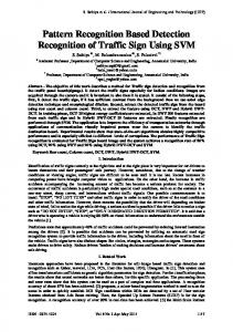
Figure 13. Precision, Precision, recall recall and and F-measure F-measure of of the the performance performance of of the the proposed proposed method method and the competing models.

According 90.67%, but According to to Figure Figure 13, 13, the the fractal fractal fuzzy fuzzy C C means means method method has has aa very very high high recall recall of of 90.67%, but the the lowest lowest precision precision of of 54.40%, 54.40%, which which leads leads to to aa small small F-measure. F-measure. The The PLSA PLSA method method has has aa low low recall recall of the F-measure F-measure is is small. small. The of 53.33%, 53.33%, and and the the precision precision is is 55.56%; 55.56%; therefore, therefore, the The SIFT SIFT matching matching method method has a moderate recall of 65.33%, but a relatively low precision of 59.04%, which also leads to has a moderate recall of 65.33%, but a relatively low precision of 59.04%, which also leads to aa small small F-measure. F-measure. The The SURF SURF matching matching method method has has aa moderate moderate precision precision of of 65.31% 65.31% and and the the lowest lowest recall recall of of 42.67%, and the F-measure is the smallest. The BOVW method has a relatively high precision of 42.67%, and the F-measure is the smallest. The BOVW method has a relatively high precision of 73.63% 73.63% and a high recall of 89.33%, so the F-measure is the second largest. Our proposed method, and a high recall of 89.33%, so the F-measure is the second largest. Our proposed method, while having while having a recall as high as the fractal fuzzy C means method, has a high precision of 89.47%, a recall as high as the fractal fuzzy C means method, has a high precision of 89.47%, which is much which is much higher than the competing methods. Therefore, the F-measure of our proposed higher than the competing methods. Therefore, the F-measure of our proposed method is the largest. method is the largest. This means that our method can not only extract semantic information to have This means that our method can not only extract semantic information to have a good representation a good representation of airports, but also highlight the difference between airports and other objects of airports, but also highlight the difference between airports and other objects effectively to avoid a effectively to avoid a relatively low precision, which is the major drawback of those competing relatively low precision, which is the major drawback of those competing methods with high recalls. methods with high recalls. In addition, we use receiver operator characteristic (ROC) curves to quantitatively compare the In addition, we use receiver operator characteristic (ROC) curves to quantitatively compare the methods’ performance. The ROC curves were generated by using the classification result of each methods’ performance. The ROC curves were generated by using the classification result of each method under different thresholds of prediction values. The prediction values range from zero to one, method under different thresholds of prediction values. The prediction values range from zero to one, and 0.5 is chosen as the threshold to distinguish between positive and negative. The ROC curves and and 0.5 is chosen as the threshold to distinguish between positive and negative. The ROC curves and the corresponding area under curve (AUC) values can illustrate the performance of our method and the corresponding area under curve (AUC) values can illustrate the performance of our method and the competing methods. In this application, we are only interested in the analysis of situations where a the competing methods. In this application, we are only interested in the analysis of situations where high true positive rate and a low false positive rate are realized at the same time, i.e., only the left part a high true positive rate and a low false positive rate are realized at the same time, i.e., only the left of the ROC curves is of practical interest to us. Therefore, according to [44,45], we compare the partial part of the ROC curves is of practical interest to us. Therefore, according to [44,45], we compare the AUC values under only a portion of the ROC curves. In the experiment, we choose the part of the partial AUC values under only a portion of the ROC curves. In the experiment, we choose the part of ROC curves corresponding to false positive rates ranging from zero to 0.1 according to the experiment the ROC curves corresponding to false positive rates ranging from zero to 0.1 according to the in [46] for the assessment of the competing methods and our proposed method. Figures 12 and 13 experiment in [46] for the assessment of the competing methods and our proposed method. show the partial ROC curves and the AUC values corresponding to false positive rates ranging from Figures 12 and 13 show the partial ROC curves and the AUC values corresponding to false positive zero to 0.1 of the methods. rates ranging from zero to 0.1 of the methods. From Figure 14, we observe that under the range of zero to 0.1 for the false positive rate, our From Figure 14, we observe that under the range of zero to 0.1 for the false positive rate, our method achieves the largest partial AUC value. We can also conclude from Figures 14 and 15 that method achieves the largest partial AUC value. We can also conclude from Figures 14 and 15 that when both the low false positive rate and the high true positive rate are required, our method can meet the requirement with the best performance. In general, all of these analyses mean that our method performs better than the competing methods.

ISPRS Int. J. Geo-Inf. 2016, 5, 115

14 of 18

when both the low false positive rate and the high true positive rate are required, our method can meet 14 of of 18 18 performance. 14

ISPRS Int. J.J. Geo-Inf. Geo-Inf. 2016, 2016, 5, 5, 115best the requirement with the ISPRS Int. 115

Figure 14. 14. Partial PartialROC ROC curves of proposed the proposed proposed method and other other methods. PLSA, probabilistic curves of the method and other methods. PLSA,PLSA, probabilistic latent Figure Partial ROC curves of the method and methods. probabilistic latent semantic semantic analysis. semantic analysis. latent analysis.

Figure 15. 15. AUC AUC of of the the proposed proposed method method and and other other methods. methods. Figure AUC of the proposed

3.2. Analyses Analyses of of the the Performance Performance of of the the Proposed Proposed Method Method on on Different Different Types Types of of Airports Airports 3.2. In general, all of these analyses mean that our method performs better than the In this thismethods. part, we we continue continue the the analysis analysis of of the the proposed proposed method. method. Recall Recall is is used used to to analyze analyze the the competing In part, proposed method’s method’s performance performance for for recognizing recognizing different different types types of of airports. airports. Table Table 11 shows shows the the total total proposed 3.2. Analyses the Performance of the Proposed Method on Different Types of Airports numbers, theofcorrectly-classified correctly-classified numbers and the corresponding corresponding recalls of different different types types of of airports airports numbers, the numbers and the recalls of in the the testing imagery. In this paper, we classify the airports in the testing imagery into two types: in testing imagery. In this paper, we classify the airports in the testing imagery into two types: In this part, we continue the analysis of the proposed method. Recall is used to analyze the Type 1 for those with runways on one side of the terminal and Type 2 for those with runways on Type 1 formethod’s those with runways onfor one side of thedifferent terminaltypes and Type 2 for those runways on proposed performance recognizing of airports. Table with 1 shows the total more than thanthe onecorrectly-classified side of of the the terminal. terminal. more one side numbers, numbers and the corresponding recalls of different types of airports in the testing imagery. In this paper, we classify the airports in the testing imagery into two types: Table 1. 1. Number Number and and recall recall of of different different types types of of airports. airports. Table

Name Total Total Number Number Correctly-Classified Correctly-Classified Number Number Recall Recall Name Type 11 60 54 90.00% Type 60 54 90.00% Type 22 15 14 94.12% Type 15 14 94.12%

ISPRS Int. J. Geo-Inf. 2016, 5, 115

15 of 18

Type 1 for those with runways on one side of the terminal and Type 2 for those with runways on more than one side of the terminal. Table 1. Number and recall of different types of airports. Name

Total Number

Correctly-Classified Number

Recall

Type 1 Type 2

60 15

54 14

90.00% 94.12%

It can be concluded from Table 1 that the proposed method does better at detecting airports with runways on more than one side of the terminal. Airports with runways on more than one side of the terminal are usually large, international airports with higher demand for land than smaller airports. They require large areas of open field, and this leads to less hybrid non-airport objects with airports. Then, the false positive rate is used to analyze what kind of non-airport objects may be more likely to be wrongly classified as airports. Table 2 shows the total numbers, the wrongly-classified numbers and the corresponding false positive rate of each type of non-airport object. In this paper, according to the analysis in Section 2.3 and the testing data, we classify the non-airport objects in the testing imagery into five classes: farmland, residential area, forest, bare land and harbor. Table 2. Number and false positive rate of different types of non-airport objects. Name

Total Number

Wrongly-Classified Number

False Positive Rate

Farmland Residential Area Forest Bare land Harbor

27 85 12 15 11

4 2 0 2 0

0.1481 0.0235 0.0000 0.1333 0.0000

From Table 2, it can be observed that farmland has the highest false positive rate, while forest and harbor have zero false positive rates. Mountain has a high false positive rate, while residential area has a low false positive rate. Airport has a high demand for open field and usually has to be located in the suburbs or even wild areas. Such areas belong to sparsely-populated residential areas, farmland or bare land, and they may be mixed with airports. 4. Conclusions VHR images have been extensively used in recent years. Recognizing and retrieving objects or scenes from VHR images is a challenging task. Among the objects that are often detected, airports play a key role because of their significance in civil and military fields. Traditional methods are ineffective; thus, a new method was proposed. The new method adapts the traditional pixel-based saliency detection method into the patch-based method for class-specific saliency to find the best segmentation to highlight the differences between airports and other objects and to analyze the spatial relationship between components of the airport to help with the abstract and detailed semantics. The new method also combines the traditional BOVW method with fractal dimension estimation, fuzzy C means clustering and image relational degree on the basis of fuzzy rule-based classification to extract the object composition for better representation of airports. The experiment proves that the proposed method outperforms the traditional methods in terms of precision and recall. However, there is still room for improvement. First, the proposed method can tell whether there is an airport in the given image or not when the airport takes up the dominant part of the image, but when an airport only takes up a small part of the given image, the method cannot tell the possible locations. Second, the proposed method can extract abstract semantics and detailed semantics from BOVW features and fractal features with analysis of the general knowledge of the airport, but lacks the

ISPRS Int. J. Geo-Inf. 2016, 5, 115

16 of 18

ability to use more specific knowledge of the airport or other mid-level or low-level features for more efficient analysis and extraction of abstract semantics and detailed semantics. Finally, the two-step classification of the proposed method should be further improved to reduce the false positive rate and to realize higher recall and precision. Therefore, for future research, we will focus on the following aspects. First, we will focus on the extraction and usage of multiple features based on more specific knowledge of the airport to express the semantic information of the airport more precisely. Second, we will propose improved saliency detection methods to extract the possible area of airports on optical imagery and present class-specific saliency more precisely. Finally, we will perform further research into the use of the image correlation degree and adapt the concept of deep learning to improve the precision and recall. Acknowledgments: This work was supported in part by the National Basic Research Program of China under Grant 2012CB719905. The authors would like to thank Xiangyun Hu of Wuhan University and. Zhaobao Zheng of Wuhan University for their valuable assistance and guidance. Author Contributions: Both authors worked on the proposal of the method and the experiment of the proposed method. The first author was involved in the design of the proposed method and the experiment data preparation. Both authors participated in the experiment and the writing of the manuscript, but the first author has taken the lead. Conflicts of Interest: The authors declare no conflict of interest.

References 1.

2. 3. 4.

5. 6.

7.

8.

9. 10. 11.

12. 13.

Gamba, P.; Dell’Acqua, F.; Lisini, G. Improving urban road extraction in high-resolution images exploiting directional filtering, perceptual grouping, and simple topological concepts. IEEE Geosci. Remote Sens. Lett. 2006, 3, 387–391. [CrossRef] Secord, J.; Zakhor, A. Tree detection in urban regions using aerial lidar and image data. IEEE Geosci. Remote Sens. Lett. 2007, 4, 196–200. [CrossRef] Sirmacek, B.; Unsalan, C. Urban area detection using local feature points and spatial voting. IEEE Geosci. Remote Sens. Lett. 2010, 7, 146–150. [CrossRef] Zuyang, K.; Zhenwei, S.; Liu, L. Airport detection based on line segment detector. In Proceedings of the 2012 International Conference on Computer Vision in Remote Sensing (CVRS), Xiamen, China, 16–18 December 2012; pp. 72–77. Huertas, A.; Cole, W.; Nevatia, R. Detecting runways in complex airport scenes. Comput. Vis. Graph. Image Process. 1990, 51, 107–145. [CrossRef] Yinwen, D.; Bingcheng, Y.; Hangyu, W.; Zhaoming, S. A runway recognition algorithm based on heuristic line extraction. In Proceedings of the 2011 International Conference on Image Analysis and Signal Processing (IASP), Wuhan, China, 21–23 October 2011; pp. 292–296. Dehong, L.; Lihan, H.; Carin, L. Airport detection in large aerial optical imagery. In Proceedings of the IEEE International Conference on Acoustics, Speech, and Signal Processing, Montreal, Canada, 17–21 May 2004; Volume 765, pp. 761–764. JunWei, H.; Lei, G.; YongSheng, B. A method of automatic finding airport runways in aerial images. In Proceedings of the 2002 6th International Conference on Signal Processing, Beijing, China, 26–30 August 2002; Volume 731, pp. 731–734. Aytekin, O.; Zongur, U.; Halici, U. Texture-based airport runway detection. IEEE Geosci. Remote Sens. Lett. 2013, 10, 471–475. [CrossRef] Chao, T.; Tan, Y.; Huajie, C.; Jinwen, T. Airport detection from large ikonos images using clustered sift keypoints and region information. IEEE Geosci. Remote Sens. Lett. 2011, 8, 128–132. Wang, X.; Wang, B.; Zhang, L. Airport detection in remote sensing images based on visual attention. In Neural Information Processing; Proceedings of the 18th International Conference, ICONIP 2011, Shanghai, China, 13–17 November 2011; Lu, B.-L., Zhang, L., Kwok, J., Eds.; Springer: Berlin, Germany, 2011; pp. 475–484. McKeown, D.M.; Harvey, W.A.; McDermott, J. Rule-based interpretation of aerial imagery. IEEE Trans. Pattern Anal. Mach. Intell. 1985, PAMI-7, 570–585. [CrossRef] Mckeown, D. Maps: The organization of a spatial database system using imagery, terrain, and map data. In Proceedings of the DARPA Image Understanding Workshop, Arlington, VA, USA, 23 June 1983; pp. 105–127.

ISPRS Int. J. Geo-Inf. 2016, 5, 115

14. 15. 16. 17. 18. 19. 20. 21. 22. 23. 24.

25.

26. 27. 28.

29. 30.

31. 32.

33.

34.

35. 36.

17 of 18

Mckeown, D. Digital Cartography and Photo Interpretation from a Database Viewpoint; Academic Press Professional, Inc.: San Diego, CA, USA, 1984. Zhao, D.; Shi, J.; Wang, J.; Jiang, Z. Saliency-constrained semantic learning for airport target recognition of aerial images. APPRES 2015, 9. [CrossRef] Wang, J.; Li, J.; Wiederhold, G. Simplicity: Semantics-sensitive integrated matching for picture libraries. IEEE Trans. Pattern Anal. Mach. Intell. 2001, 23, 947–963. [CrossRef] Smeulders, A.W.M.; Worring, M.; Santini, S.; Gupta, A.; Jain, R. Content-Based Image Retrieval at the End of the Early Years. IEEE Trans. Pattern Anal. Mach. Intell. 2000, 22, 1349–1380. [CrossRef] Ma, H.; Zhu, J.; Lyu, M.R.T.; King, I. Bridging the semantic gap between image contents and tags. IEEE Trans. Multimed. 2010, 12, 462–473. [CrossRef] Tang, J.; Zha, Z.J.; Tao, D.; Chua, T.S. Semantic-Gap-Oriented Active Learning for Multilabel Image Annotation. IEEE Trans. Image Process. 2012, 21, 2354–2360. [CrossRef] [PubMed] Zhang, L.; Shum, H.P.; Shao, L. Discriminative Semantic Subspace Analysis for Relevance Feedback. IEEE Trans. Image Process. 2016, 25, 1275–1287. [CrossRef] [PubMed] Alexe, B.; Deselaers, T.; Ferrari, V. What is an object? In Proceedings of the 2010 IEEE Conference on Computer Vision and Pattern Recognition, San Francisco, CA, USA, 13–18 June 2010; pp. 73–80. Goferman, S.; Zelnik-Manor, L.; Tal, A. Context-aware saliency detection. IEEE Trans. Pattern Anal. Mach. 2012, 34, 1915–1926. [CrossRef] [PubMed] Liu, T.; Yuan, Z.; Sun, J.; Wang, J.; Zheng, N.; Tang, X.; Shum, H.Y. Learning to detect a salient object. IEEE Trans. Pattern Anal. Mach. Intell. 2011, 33, 353–367. [PubMed] Yang, C.; Zhang, L.; Lu, H.; Ruan, X.; Yang, M.H. Saliency detection via graph-based manifold ranking. In Proceedings of the 2013 IEEE Conference on Computer Vision and Pattern Recognition, Portland, OR, USA, 23–28 June 2013; pp. 3166–3173. Linfeng, X.; Hongliang, L.; Zhengning, W. Saliency detection from joint embedding of spatial and color cues. In Proceedings of the 2012 IEEE International Symposium on Circuits and Systems, Seoul, Korea, 20–23 May 2012; pp. 2673–2676. Fan, Z.; Bo, D.; Liangpei, Z. Saliency-guided unsupervised feature learning for scene classification. IEEE Trans. Geosci. Remote Sens. 2015, 53, 2175–2184. Yao, X.; Han, J.; Guo, L.; Bu, S.; Liu, Z. A coarse-to-fine model for airport detection from remote sensing images using target-oriented visual saliency and CRF. Neurocomputing 2015, 164, 162–172. [CrossRef] Feifei, L.; Perona, P. A bayesian hierarchical model for learning natural scene categories. In Proceedings of the 2005 IEEE Computer Society Conference on Computer Vision and Pattern Recognition, San Diego, CA, USA, 20–25 June 2005; pp. 524–531. Bosch, A.; Zisserman, A.; Muoz, X. Scene classification using a hybrid generative/discriminative approach. IEEE Trans. Pattern Anal. Mach. Intell. 2008, 30, 712–727. [CrossRef] [PubMed] Sivic, J.; Zisserman, A. Video google: A text retrieval approach to object matching in videos. In Proceedings of the Ninth IEEE International Conference on Computer Vision, Nice, France, 13–16 October 2003; Volume 1472, pp. 1470–1477. Lowe, D.G. Distinctive image features from scale-invariant keypoints. Int. J. Comput. Vis. 2004, 60, 91–110. [CrossRef] Philbin, J.; Chum, O.; Isard, M.; Sivic, J.; Zisserman, A. Object retrieval with large vocabularies and fast spatial matching. In Proceedings of the 2007 IEEE Conference on Computer Vision and Pattern Recognition, Minneapolis, MN, USA, 17–22 June 2007; pp. 1–8. Pedrosa, G.V.; Traina, A.J.M.; Traina, C. Using sub-dictionaries for image representation based on the bag-of-visual-words approach. In Proceedings of the 2014 IEEE 27th International Symposium on Computer-Based Medical Systems, New York, NY, USA, 27–29 May 2014; pp. 165–168. Rocha, B.M.; Nogueira, E.A.; Guliato, D.; Ferreira, D.L.P.; Barcelos, C.A.Z. Image retrieval via generalized i-divergence in the bag-of-visual-words framework. In Proceedings of the 2014 21st IEEE International Conference on Electronics, Circuits and Systems (ICECS), Marseille, France, 7–10 December 2014; pp. 734–737. Nagarajan, G.; Minu, R. Fuzzy ontology based multi-modal semantic information retrieval. Procedia Comput. Sci. 2015, 48, 101–106. [CrossRef] Su, J.; Wang, B.; Hsu, T.; Chou, C.; Tseng, V. Multi-modal image retrieval by integrating web image annotation, concept matching and fuzzy ranking techniques. Int. J. Fuzzy Syst. 2010, 12, 135–149.

ISPRS Int. J. Geo-Inf. 2016, 5, 115

37. 38. 39. 40. 41.

42.

43. 44. 45.

46.

18 of 18

Athanasiadis, T.; Mylonas, P.; Avrithis, Y.; Kollias, S. Semantic image segmentation and object labeling. IEEE Trans. Circuits Syst. Video Technol. 2007, 17, 298–312. [CrossRef] Zhaobao, Z.; Li, P.; Hong, Z. Application of Image Correlation Degree to Image Fuzzy Classification. Geomat. Inf. Sci. Wuhan Univ. 2015, 40, 574–577. (In Chinese) Li, J.; Du, Q.; Sun, C. An improved box-counting method for image fractal dimension estimation. Pattern Recognit. 2009, 42, 2460–2469. [CrossRef] Xuanli Lisa, X.; Beni, G. A validity measure for fuzzy clustering. IEEE Trans. Pattern Anal. Mach. Intell. 1991, 13, 841–847. Hofmann, T. Probabilistic latent semantic indexing. In Proceedings of the 22nd Annual International ACM SIGIR Conference on Research and Development in Information Retrieval, Berkeley, CA, USA, 15–19 August 1999; ACM: New York, NY, USA; pp. 50–57. Zhou, Z.; Zang, Y.; Li, Y.; Zhang, Y.; Wang, P.; Luo, X. Rice plant-hopper infestation detection and classification algorithms based on fractal dimension values and fuzzy c-means. Math. Comput. Model. 2013, 58, 701–709. [CrossRef] Bay, H.; Ess, A.; Tuytelaars, T.; Van Gool, L. Speeded-up robust features (surf). Comput. Vis. Image Underst. 2008, 110, 346–359. [CrossRef] Dodd, L.; Pepe, M. Partial auc estimation and regression. Biometrics 2003, 59, 614–623. [CrossRef] [PubMed] He, Y.; Escobar, M. Nonparametric statistical inference method for partial areas under receiver operating characteristic curves, with application to genomic studies. Stat. Med. 2008, 27, 5291–5308. [CrossRef] [PubMed] Mcclish, D. Analyzing a portion of the ROC curve. Med. Decis. Mak. 1989, 9, 190–195. [CrossRef] © 2016 by the authors; licensee MDPI, Basel, Switzerland. This article is an open access article distributed under the terms and conditions of the Creative Commons Attribution (CC-BY) license (http://creativecommons.org/licenses/by/4.0/).