Automatic Rate Adaptation
∗
Aditya Gudipati, Sachin Katti
[email protected],
[email protected]
Information Systems Lab, Stanford University, Stanford, CA, USA Abstract
sharp all or nothing behavior, i.e. each bitrate has a SNR Rate adaptation is a fundamental primitive in wireless net- threshold below which most of the data bits cannot be corworks. Since wireless channel strength varies quickly and un- rectly decoded, but above that threshold very likely the entire predictably, senders have to constantly measure the channel packet gets decoded. The rate adaptation problem is thus to pick the bitrate that and correspondingly adapt the bitrate so that the transmitted adds the minimal protection necessary to ensure the packet packet gets correctly decoded. Prior approaches to this probgets delivered reliably and thus maximizes throughput. Howlem can be divided into two classes: those that require conever, since the wireless channel condition fluctuates constantly, stant and expensive feedback from the receiver about channel and often unpredictably, the sender has to measure the channel strength, or those that use coarse and often inaccurate inferSNR, and correspondingly adjust the bitrate it uses. A large ence based on packet losses to measure channel strength and and growing body of prior work exists on this problem, and the decide what bitrate to use. proposed techniques can be divided into two approaches: ones In this paper we take the opposite approach. Instead of acthat use direct feedback from the receiver about the channel tively adapting the bitrate based on receiver or packet loss SNR [2, 13], or ones that infer channel strength based on past feedback, we present a technique where the sender does no patterns of packet delivery successes [1, 4, 9, 6]. The first apmeasurement or adaptation, yet the receiver manages to reproach requires expensive and constant feedback, and can still ceive packets at a bitrate corresponding to whatever channel be inaccurate because channel conditions can change since the conditions exist at that point. The technique works with exfeedback was received. The second approach requires expenisting coding and modulation techniques (e.g. convolutional sive probing, and the inferred channel strength can be wildly codes in WiFi), and requires no changes to them. Our preliminaccurate since packet delivery is a very coarse measure. inary evaluation shows that our proposed feedback-free techIn this paper, we take the opposite approach. We present a nique achieves a performance that is nearly as good as if the technique, Automatic Rate Adaptation (ARA), where instead sender knew exactly what the channel strength was in advance. of performing any complicated probing or obtaining channelstate feedback from the receiver, we show that a sender can Categories and Subject Descriptors achieve almost the optimal bitrate adaptation possible by usC.2.1 [Computer Communication Networks]: Wireless com- ing a single novel transmission algorithm. The sender simply munication transmits packets using our fixed algorithm, and does not need to change it in any way due to packet delivery success/failure. The receiver recovers whatever packets it can using our proGeneral Terms posed decoding algorithm and sends a simple feedback in the Performance, Reliability, Design form of an ACK when it is finished decoding. We show that this simple scheme achieves the same bitrate as the optimal 1. INTRODUCTION scheme, i.e. a scheme where the sender knows exactly what To communicate reliably on a wireless link, a sender has to the channel SNR is in advance, and picks the optimal bitrate protect his data bits against link impairments such as attenu- to transmit at that SNR. ation, fading and noise. Data protection is added via a comThe key technique behind ARA is the concept of a minbination of channel coding and modulation schemes, which imum distance transformer (MDT). The technique is based together dictate the achieved bitrate. For example, a 1Mbps on the observation that for any combination of channel code bitrate (the lowest WiFi bitrate) is due to the choice of a very and modulation scheme to work (i.e. decode reliably), the redundant channel code and a very sparse modulation scheme minimum distance between nearby constellation points in the (QPSK). Naturally, this bitrate is the most protected and works modulation scheme must be above a threshold to tolerate diswell at low SNR, higher bitrates offer less protection and can- tortion due to noise. The threshold is a function of channel not be decoded at low SNR. In fact, these bitrates exhibit a SNR and the redundancy in the channel code. If the modulation scheme’s minimum distance is above that threshold, ∗ Permission to make digital or hard copies of all or part of this work for personal or classroom use is granted without fee provided that the channel code can correct any residual errors. With curcopies are not made or distributed for profit or commercial advantage rent techniques, the minimum distance is fixed and dictated by and that copies bear this notice and the full citation on the first page. the choice of the modulation scheme and transmission power. To copy otherwise, or republish, to post on servers or to redistribute ARA designs and develops a novel minimum distance transto lists, requires prior specific permission and/or a fee. formation (MDT) technique that automatically adjusts the minHotnets’10, October 20–21, 2010, Monterey CA, USA imum distance, such that it is sufficient for the channel code c Copyright 2010 ACM 978-1-4503-0409-2/10/10...$10.00
we picked to decode. Specifically, instead of directly trans- completely new hardware encoders and decoders, and also are mitting conventionally modulated symbols (e.g. QPSK sym- optimized to work in the low SNR regimes typical of cellular bols), we transmit random complex linear combinations of a wireless channels. Our technique works with existing channel batch of them. The intuition is that when we take a batch of codes, and can work over both low and high SNR conditions. L conventional symbols, and transmit M linear combinations of them, in essence we are mapping points from a L dimen- 3. OVERVIEW sional space (the conventional symbols) to points in a M diSenders have to adapt transmissions rates because of the mensional space. Depending on the relative values of M and threshold behavior of conventional techniques, i.e. they deL, the minimum distance in this new space can be controlled. code only at or above a particular SNR threshold depending on Thus a sender, can transmit random linear combinations until the channel coding rate and modulation choice. Even though the minimum distance in the new space goes above the threshit is fairly introductory material, we first discuss the reasons old required by the channel code to decode correctly. Morefor this thresholding behavior since it provides insight into our over, the adjustment happens without any channel-state feedeventual design. back, thus achieving the desired automatic rate adaptation. In current schemes, data bits are first channel coded to add A key feature of ARA is that it works with existing moduprotection against noise. The level of protection is parameterlation and coding schemes and requires no changes to them. ized by the coding rate (e.g a 1/2 rate code implies that every Second, ARA is orthogonal to the choice of coding and moddata bit is protected with one extra bit of redundancy). Coded ulation schemes, i.e. it achieves close to the best performance bits are then modulated, i.e. they are mapped to points in a possible with whatever coding and modulation schemes are complex constellation and transmitted on the wireless chanavailable. This implies that any future benefits from advances nel. For example in BPSK, √ bits are mapped to two points √ in coding and modulation techniques are immediately accesP , − P ) (P is the transmission power) on the real line ( sible with ARA. and transmitted. Due to attenuation and additive noise the reWe evaluate ARA on wireless channels with SNRs that vary ceiver gets y = s + n, where n is Gaussian noise with varifrom 5-20dB (the range typically observed in WiFi channels) 2 ance σ . When decoding, the receiver first demodulates the and compare it to the optimal omniscient rate adaptation scheme, received symbol, i.e. maps it to the nearest constellation point i.e. the one where the sender has instantaneous and perfect Hence √ if the Gaus√ information of the channel SNR at any instant and picks the and infers what coded bit was transmitted. P / − P ) the receiver sian noise value is greater/less than ( corresponding best bitrate. The simulation results suggest that makes a bit error. However, the channel code decoder can corour technique achieves a performance that is within 10% of the rect a certain number of errors (depending on the amount of performance of the optimal scheme. These results are prelimredundancy added) and decode the final data. Thus as long as inary, and we expect that the performance will improve even the number of bit flips at the demodulation (BPSK) stage are further with refinements of the decoding technique. less than the correcting power of the channel code, the data eventually gets decoded correctly. 2. RELATED WORK Assuming the channel code rate is fixed, the key to ensuring decoding success is to make sure that the demodulation Prior work on rate adaptation is based on estimating the stage does not make more bit errors than the channel code can channel strength via direct SNR feedback from the receiver, or handle. This error rate is dictated by the minimum distance√beinferring based on packet delivery success/failures [2, 13, 1, 4, tween any two constellation points (e.g. for BPSK it is 2 P ) 9, 6]. SNR feedback in fast changing mobile channels can be and how it compares with the noise power (σ 2 ). To get good expensive, and worse inaccurate, since by the time the transmitter uses the feedback, the channel might have changed. In- performance, the the minimum distance has to be sufficiently ference based on packet delivery success can be highly inaccu- large so that no more than the tolerable number of bit errors rate, since packet delivery is a very coarse measure of channel occur. If its too small, the channel code cannot correct, if its strength, and can be distorted by factors such as collisions, not too large, the extra redundancy in the channel code is wasteful. just channel fluctuations. ARA avoids all these complications Modulation schemes have different minimum distances (e.g. since it requires neither channel-state feedback nor inference. BPSK, QPSK, 16-QAM, 64-QAM have successively decreasARA is related to prior work in rateless codes and hybrid ing minimum distances), and depending on the channel SNR ARQ. Rateless codes such as LT [8], Raptor codes [10] al- the rate adaptation module’s job is to pick the combination low one to automatically achieve the capacity of an erasure of modulation and channel coding that correctly decodes and channel without knowing the packet loss probability in ad- maximizes throughput. Figure 1 demonstrates this thresholdvance. However these techniques work with erasure channels ing behavior by plotting the SNR thresholds at which different only, and have poor performance for channels with noise [10] combinations of channel codes and modulation schemes begin (such as wireless channels). Our technique works with noisy to decode. channels. Second, hybrid ARQ schemes used in 4G wireless systems based on punctured turbo codes [7, 11] do adapt to 3.1 Our Approach Our goal is to automatically obtain the maximum bitrate the minor misestimations of the SNR by transmitting punctured bits if the packet is not decoded in the first transmission. But channel supports, without knowing the channel SNR in adthey do not provide a infinite stream of bits and hence cannot vance. In our approach, the channel code and modulation are adapt over the entire SNR range. Also, these schemes require fixed and do not adapt to channel SNR. Through the rest of
1
Decoding probability
0.9 0.8
16−QAM 16−QAM 64−QAM 64−QAM
Data
1/2coderate 2/3coderate 1/2coderate 2/3coderate
Channel Code
Coded Data bits
Modulator
Coded Data Symbols
MDT Encoding
Channel
0.7 0.6 0.5
Soft Decoder for Channel Code
0.4
Soft Info on bits
Soft Info on symbols
Demodulator
MDT Decoder
0.3
Decoded bits
0.2
Decoded symbols
Modulator
0.1 0 5
10
15
20
SNR
Figure 1: Thresholding Behaviour at different channel codes and modulation schemes this section, we will assume that input data has already been passed through a channel coder and modulator to produce a stream of complex symbols s (of unit average power) that have to be transmitted using at most power P . We will also assume that the Gaussian noise variables n have a fixed variance of σ 2 that is unknown to the sender. Finally, we assume that the channel attenuation has been normalized to 1 and any attenuation has been accounted for by adjusting the noise power. The key idea behind our approach is the concept of a minimum distance transformer (MDT). Intuitively, a MDT takes a batch of modulated symbols and maps them to a different space where the minimum distance between the √ two closest points in the original modulation scheme (e.g. 2 P in BPSK) can be tuned to meet the channel code’s requirements. To understand how MDT works, we begin with a simple (but suboptimal) approach that demonstrates the basic idea. Assume we have a modulated BPSK symbol s. A simple approach to amplify the minimum distance is to take the symbol s, and transmit it multiple (M ) times, but multiply each transmission by a complex number of unit magnitude but random phase ri = ejθi (so transmission power does not change). The receiver therefore gets the following symbols after noise gets added √ ~x = ~r P s + ~n (1) where ~r is the M length vector of random complex numbers formed by the coefficients of each transmission, and ~n is the noise vector for the M transmissions. The transmitter in essence has mapped a simple BPSK symbol s to a random point ~x in a M -dimensional space. To see why this amplifies minimum distance, lets compute the Euclidean distance in this new√space√between the original two BPSK points√ P , − P . The new distance is √ constellation √ ||2 P ~r|| = 2 P ||~r|| = 2 M P ( since all the√ entries of ~r are unit magnitude complex numbers ), which is M times the original minimum distance, providing much higher resilience to noise. At some value of M (i.e. after a certain M number of transmissions), the channel code will meet its minimum distance threshold and be able to decode. As the reader can tell, the above naive approach is quite inefficient. It increases the minimum distance in large increments, whereas the channel code itself might need a much smaller increment. Our key observation is that instead of operating over single symbols as above, we can spread the transmission power over the symbols belonging to a batch of modulated symbols, say L, by transmitting a random linear combi-
Figure 2: ARA’s overall architecture nation of them. Specifically, what we transmit on the channel is the following ! i=L X p (2) ri si x = (P/L) i=1
The transmitter thus sends M such linear combinations, and the receiver receives the following system of linear equations distorted by noise. p (3) ~y = ~x + ~n = (P/L)R~s + ~n
where ~s is the L length vector corresponding to a batch of L modulated symbols, R is the M × L matrix consisting of the random phase coefficients ri defined above, and all the other definitions are the same. To understand how this technique achieves minimum distance transformation, we can use the following visualization. Intuitively, this operation is taking L dimensional vectors ~s and mapping it to random points in a M dimensional space. As M increases, the minimum distance between the two closest points in this new p space increases. When M = 1 the minimum distance is 2 P/L. For any value M , the minimum distance between points in the M -dimensional space corresponding to the closest constellationp points for modulated symbol p si (assuming BPSK) is ||2R(i) P/L|| = 2 M P/L, where R(i) is the i’th column of matrix R. Thus the minimum distance increases monotonically with M . Hence, by controlling the value of M (i.e. by controlling the number of transmissions), we can control the minimum distance until the fixed channel code’s requirements are met and it can decode. Thus, we can keep on transmitting linear combinations until all the L modulated symbols can be decoded, achieving the automatic rate adaptation property. Figure 5 shows a simplified example of MDT for transmitting L = 2 BPSK symbols, and how the minimum distance improves with each transmission M = 1, 2, 3. To decode, the receiver has to estimate what are the likely modulated symbols ~s given ~y , the matrix R and an estimate of the noise power σ 2 . This is a well known problem in coding theory, called lattice decoding [12] that has applications in a wide range of communication scenarios (e.g. MIMO). The key intuition behind the decoding algorithm is the same as our visualization above, the matrix R defines a random mapping of L dimensional vectors to points in a M dimensional space (defined as a lattice in the coding theory literature). The decoding problem finds the nearest lattice point (~x) to the received point ~y , and from there decodes the corresponding ~s. We leverage existing fast lattice decoding algorithms to imple-
L Data Blocks
Coded Data symbols (si)
Multiply each column by
R Channel Code & Modulation
Packets containing Linearly combined Data symbols (xi)
the following operation xji = r~j s~i T M
M
L
Figure 3: ARA’s encoding process Possible points (in M-dimensional space) Received point
R
Sphere
where s~i signifies the transposed vector, and r~j is a random complex vector of length L, with each of the entries having unit magnitude but random phase. This process is repeated with the same r~j for all the n symbols, these n linear combinations are then transmitted as a packet.The subscript j corresponds to the fact that this linear combination belongs to the j’th transmitted packet. We can generate as many packets as we like, with each packet being generated by a different complex random vector ~r having unit magnitude entries. The process stops only when the receiver has managed to decode all L modulated packets and sends an ACK saying so, and then the sender moves on to the next batch. The complex number xji is scaled up by the AGC to whatever is the transmit power constraint. Figure 3 depicts the MDT encoding process.
4.2 Figure 4: Sphere Decoding ment the above intuition efficiently. We describe the encoding and decoding algorithms in more detail in Section 4. Figure 2 shows the high level flow of our encoding and decoding algorithms. Finally, a further refinement is possible that significantly improves the performance of our approach. Since the components of ~s belong to separate channel coded and modulated blocks, we do not need to wait for all the modulated symbols in ~s to be decoded exactly. Instead as soon as one modulated symbol (lets say s1 ) can be decoded (i.e. the first row of symbols in Fig. 3) can be decoded, the correct value of s1 can be subtracted from ~y to get a new system of linear combinations which is easier to decode. Thus we can iteratively cancel out any symbol that is decoded, and improve the decoding performance for the undecoded symbols.
4. DESIGN AND ANALYSIS In this section we describe the design of the encoder and decoder. We focus on the high level aspects of the design, and refer the reader to appropriate references when we reuse algorithms from existing communication theory literature.
4.1 Sender The sender encodes his data in three steps: (1) Divide data into a batch of L blocks, and pass each block through fixed channel encoders to produce L coded blocks. (2) Modulate the coded bits for transmission, i.e. map the coded bits to appropriate points in the constellation (e.g. 1 → 1, 0 → −1 in BPSK) to produce L packets of n modulated symbols each. (3) Pass the L modulated packets through the MDT component. As explained in Section 3, MDT creates random complex linear combinations of modulated symbols. Specifically, MDT takes the i’th complex symbol in each of the L modulated packets, and forms a L-dimensional complex vector, s~i . It then creates a single complex random linear combination via
(4)
T
Receiver
The receiver gets distorted and attenuated symbols after they pass through the wireless channel. It waits to receive enough linear combinations until it can decode the original data. Assuming it needs M linear combinations to decode, the received symbols can be written as y~i = x~i + ~n = R~ si + ~n
(5)
The rows of the M × N sized matrix R are the M random complex vectors r~j , j ∈ {1, . . . , M } used in producing the linear combinations. The decoding proceeds at a high level in two steps (a) First, decode the MDT stage, i.e., find the vector of modulated symbols s~i given that we received y~i . (b) Next, each of the L modulated packets are decoded using conventional demodulation and channel decoding. This works exactly as in current hardware, hence we focus on Step 1 below. The key problem in the MDT stage is to find the vector s~i that is most likely given we received y~i . As we discussed before, the MDT encoding can be visualized as mapping each possible L length vector s~i to a unique but random discrete point x~i in a M dimensional space. The collection of all the possible discrete points in the M dimensional space is called a lattice [12]. After going through the wireless channel, this point is distorted by noise and attenuation, and hence we receive y~i = x~i + ~n . Thus, the received point y~i will likely still be close to the point (in a Euclidean distance sense) in the lattice (x~i ) that was transmitted, with the actual distance being determined by the noise power. Based on this intuition, this part of the decoding algorithm has to accomplish two things. First, it has to find the discrete points x~i in the lattice closest to the received point y~i . Second, among all these possible choices for x~i and the corresponding possible modulated symbol vectors s~i , it has to find the correct s~i . This is a well known problem in communication theory, known as lattice decoding [12]. Sphere decoding is a standard and well known technique to solve this problem, which we use in MDT too. For a detailed description of this algorithm we refer the reader to [5], here we give an intuitive description of the algorithm as applied to ARA.
1.5
nd
2
Tx
(1,1)↔(1.34,1.34)
1
0.5
rd
1.5
Dist.=2
1
(−1,1)↔(−0.45,0.45)
Dist.=2 Dist.=1.26
Dist.=2.68
Dist.=2.19 0.5
st
1 Tx
0
nd
2
0
Dist.=2
(1 , 1)↔(1.34 , 1.34 , −0.45)
Tx
st
1 Tx
−0.5
0.5
3 Tx (−1 , 1)↔(−0.45 , 0.45 , 1.34)
(1,−1)↔(0.45,−0.45)
Dist.=2
−0.5
Dist.=2.68
(−1 , −1)↔(−1.34 , −1.34 , 0.45)
Dist.=2.19
−1
Dist.=0.89
Dist.=0.89
−1
Dist.=0.89
0
(−1,−1)↔−1.34
(1,−1)↔0.45
−1.5
−1
−0.5
0
(−1,−1)↔(−1.34,−1.34) −1.5 −1.5
(1,1)↔1.34
(−1,1)↔−0.45 −0.5 −2
0.5
(a) 1 transmission
−1.5
1
1.5
−1
−0.5
1
0
0.5
1
1.5
0
(1 , −1)↔(0.45 , −0.45 , −1.34) −1
−1.5
−1
−0.5
0
0.5
1
1.5
2
(b) 2 transmissions
(c) 3 transmissions
Figure 5: Minimum distance increases from 0.89 to 1.26 to 2.19 with consecutive transmissions. At each instance, the sender transmits a random linear combination of 2 BPSK symbols
4.2.1
Sphere Decoding
The basic idea behind sphere decoding is that instead of attempting to search over the entire lattice (i.e. the set of all possible points that are exponential in number), we can restrict our search to a sphere of a fixed radius around the received point y~i , thereby reducing the search space and hence complexity. Figure 4 demonstrates the process. Clearly, the closest lattice point in the sphere will also be the closest point for the whole lattice. Sphere decoding thus has to address two main questions (a) What should be the radius of the sphere within which we look for lattice points? If the radius is large, we may obtain too many points, if its small, we may obtain no points. The right answer actually depends on the noise power in the channel. The radius of the sphere should at least be the standard deviation in the Gaussian noise. To be safe, ARA picks three times the standard deviation of the noise as the radius in each dimension of the vector to ensure that we do not miss any likely candidates. (b) Second, once the radius has been picked, how to tell what lattice points actually lie inside this sphere? If this requires testing the distance to y~i from every lattice point, then there is no point in sphere decoding as we will need an exhaustive search. Fortunately, there is an efficient way to solve this problem. Although it is difficult in general to determine the lattice points in a M -dimensional sphere, it is trivial to do so on the one dimensional case when M = 1. The reason is that searching on a single dimension reduces to a simple binary search procedure, that can be easily accomplished. We can use this procedure to go from the k’th dimension to the k + 1’th dimension, because if we have determined all the kdimensional points that lie in the sphere, then for any such point, the set of admissible values in the k + 1’th dimensional coordinate can be found using a simple binary search. The above naturally suggests the algorithm, start with a single dimension and successively add dimensions to it until we cover all M dimensions. The above algorithm sketch is intentionally high-level due to space constraints. However, sphere decoding by itself is a well understood topic, and we refer the reader to [5] for a detailed survey. In our implementation we use the algorithm described in Section 3 of [5].
4.2.2
Iterative Decoding
Sphere decoding gives a rough estimate of the likely lattice points and corresponding possible values of the modulated symbol vector s~i that were transmitted. However to decode the actual data transmitted, we have to use the conventional demodulator and channel decoder. Specifically, from each received vector y~i , we get a list of candidate modulated symbol vectors s~i that could have been transmitted. Each component in these vectors corresponds to a different data block, that has been separately channel coded and modulated. Now the channel code takes these likely estimates and attempts conventional soft decoding [3]. It repeats the process for all L batches, and if all of them are successfully decoded, an ACK is sent. If not, we wait to receive another packet, and retry the same process. We can exploit the channel decoding stage to further improve the accuracy of the sphere decoding stage. The key idea is that after the channel code has managed to decode at least one symbol in s~i , we can take the correct estimate for the corresponding modulated symbol, and subtract it from y~i . This reduces the uncertainty in the estimates for the other symbols, since each component of s~i acts as interference to the other components. Exactly decoding and subtracting any one of them, automatically reduces the perceived interference to the other components, and helps kickstart their decoding.
5.
EVALUATION
Compared Schemes & Metric: We compare our approach against the optimal conventional rate adaptation scheme, i.e., one where the sender has perfect omniscient knowledge of the instantaneous channel SNR, and picks the channel coding and modulation scheme that maximizes throughput. The metric for comparison is throughput defined as the data rate achieved in bits/second/Hz (b/s/Hz). We assume AWGN channels and carry out our simulations on MATLAB. At each SNR value, the ARA is simulated 10 times and the throughputs are averaged and plotted (error bars indicate the standard deviation). For our scheme, we use a batch size L of 8, and the channel code is fixed to a convolutional code of rate 2/3 and the modulation scheme is fixed to QPSK, and not allowed to change with SNR. The conventional optimal scheme has a choice of channel coding rates 1/4, 1/3, 1/2, 2/3 and modulation schemes
Achieved throughput (in bits/second/Hz)
4
3.5
Optimal Rate Adaptation Scheme ARA
3
2.5
2
1.5
1
0.5 4
6
8
10
12
14
16
18
20
SNR(in dB)
Figure 6: Comparison of throughputs. ARA achieves almost the same performance as the optimal conventional rate adaptation scheme without requiring any channelstate feedback. 12
Average LLR
10
8
SNR= 5dB SNR= 7dB SNR= 9dB SNR= 10dB 95% Decoding proababilty
6.
6
4
2
0 0
2
4
ratio (LLR) for each symbol, and signifies the confidence the MDT component has in its decoding decision for each symbol. Typically for any channel code, there is a threshold LLR (depending on the channel coding rate) above which the channel decoder can decode the final data bits. Figure 7 plots the evolution of this soft information with the number of received transmissions per batch of symbols (the batchsize is 8) at four different channel SNRs until a packet gets decoded. The threshold for the channel code to decode is an LLR of 8 (LLR follows a logarithmic scale and varies between -100 to 100, with 100 representing perfect decoding). As we can see, with increasing number of receptions, the LLR of the symbols decoded by MDT improves, and after it crosses the threshold required, the fixed channel code immediately decodes. The number of receptions required depends on the instantaneous channel SNR, with lower SNRs requiring more receptions.
6
8
10
12
14
Transmissions (until start of decoding)
Figure 7: Evolution of average LLRs with the number of transmissions at different SNRs (QPSK, 8-PSK, 16-QAM and 64-QAM) that are used in current WiFi systems, and picks the best combination for any SNR. (a) Benchmark Results: First, we study how our approach for automatic rate adaptation compares with the optimal conventional rate adaptation scheme. The experiment is run as follows: we run experiments for SNRs between 5-20 dB in increments of 1dB, and for each SNR, the optimal scheme picks the best channel coding and modulation scheme, while ARA is unaware of the SNR and uses the fixed channel code and modulation scheme decided above. Each experiment is repeated 10 times and the results are averaged. Figure 6 plots the average bits/second/Hz achieved by the two schemes. The figure shows that ARA achieves a performance that is almost as good as the optimal scheme. For most of the SNR range between 5-16 dB, the achieved throughput is almost the same as the optimal scheme. For higher SNRs above 16dB, the performance is worse by 10%. The dropoff is thus small, but we believe even this dropoff can be eliminated. Specifically, at such high SNR, the packets are getting decoded with very few linear combinations, typically 3 − 4. At such low numbers, the random design of the matrix R in the MDT component can be slightly sub-optimal (in terms of how the minimum distances scale). A more careful choice we believe will eliminate even the small 10% inefficiency, allowing ARA to trace the optimal scheme in the entire SNR range. (b) Soft Information Evolution: To understand how ARA achieves automatic rate adaptation, we plot the evolution of the soft information for each modulated symbol in the batch of L streams. Soft information is defined as the log likelihood
CONCLUSION
In this paper, we have described a novel technique ARA that can automatically achieve the best bitrate at any channel SNR, without requiring any channel-state feedback or adaptation. The design of ARA is modular, i.e. it can work with any existing channel coding and modulation schemes without requiring any changes to them. We believe that ARA has the potential to greatly simplify the design of the wireless PHY, by reducing the overhead of co-ordination needed for rate adaptation and eliminating expensive retransmissions needed due to incorrect bitrate choices. ARA naturally lends itself to a number of future research avenues. First, we are currently working on a linear time decoding algorithm. Second, we plan to explore how ARA can be applied to scenarios in opportunistic routing, relaying and graceful video delivery (since all of them aim to exploit partially correct packets to improve performance). Finally, we plan to implement ARA on a USRP2 platform, and test it in complex time-varying channels such as outdoor mobile wireless scenarios.
7.
REFERENCES
[1] J. Bicket. Bit-rate selection in wireless networks. MS Thesis, Massachusetts Institute of Technology, 2005. [2] J. Camp and E. Knightly. Modulation rate adaptation in urban and vehicular environments:cross-layer implementation and experimental evaluation. In ACM MOBICOM, 2008. [3] J. Hagenauer and P. Hoeher. A viterbi algorithm with soft-decision outputs and its applications. In Proc. of GLOBECOM, 1989. [4] G. Judd, X. Wang, and P. Steenkiste. Efficient channel-aware rate adaptation in dynamic environments. In ACM MOBISYS, 2008. [5] T. Kailath, H. Vikalo, and B. Hassibi. Mimo receive algorithms. Space-Time Wireless Systems: From Array Processing to MIMO Communications, 2005. [6] A. Kamerman and L. Monteban. Wavelan r-ii: A high-performance wireless lan for the unlicensed band. Bell Labs Technical Journal, 2, 1997. [7] S. Lin and P. Yu. A hybrid arq scheme with parity retransmission for error control of satellite channels. IEEE Trans. on Communications, 1982. [8] M. Luby. Lt codes. In Proc. of FOCS 2002, 2002. [9] MadWiFi. Onoe rate control. http://madwifi.org/browser/trunk/ath_rate/onoe. [10] A. Shokrollahi. Raptor codes. IEEE/ACM Trans. Netw., 14(SI):2551–2567, 2006. [11] E. Soljanin, R. Liu, and P. Spasojevic. Hybrid arq in wireless networks. In DIMACS Workshop on Networking, 2003. [12] E. Viterbo and J. Boutros. A universal lattice code decoder for fading channels. IEEE Transactions on Information Theory, 1999. [13] M. Vutukuru, H. Balakrishnan, and K. Jamieson. Cross-layer wireless bit rate adaptation. In ACM SIGCOMM, Barcelona, Spain, August 2009.