Automatic recognition of harmonic bird sounds using a ... - CiteSeerX

Automatic recognition of harmonic bird sounds using a frequency track extraction algorithm

Jason R. Heller Dept. Applied Math. and Stat.,Stony Brook University, NY John D. Pinezich Advanced Acoustic Concepts, Inc., Hauppauge, NY

1

Abstract This paper demonstrates automatic recognition of vocalizations of four common bird species (herring gull [Larus argentatus], blue jay [Cyanocitta cristata] , Canada goose [Branta canadensis], and American crow [Corvus brachyrhynchos]) using an algorithm that extracts frequency track sets using track properties of importance and harmonic correlation. The main result is that a complex harmonic vocalization is rendered into a set of related tracks that is easily applied to statistical models of the actual bird vocalizations. For each vocalization type, a statistical model of the vocalization was created by transforming the training set frequency tracks into feature vectors. The extraction algorithm extracts sets of frequency tracks from test recordings that closely approximate harmonic sounds in the file being processed. Each extracted set in its final form is then compared with the statistical models generated during the training phase using Mahalanobis distance functions. If it matches one of the models closely, the recognizer declares the set an occurrence of the corresponding vocalization. The method was evaluated against a test set containing vocalizations of both the four target species and sixteen additional species as well as background noise containing planes, cars, and various natural sounds.

2

I. INTRODUCTION

An important application of automated bird sound recognition is as an aid to mitigating bird-aircraft strike hazards (BASH). There are more than 10000 reported collisions of aircraft with birds every year costing more than $100 million in damage and canceled or delayed flights1 . The US Air Force has implemented a program called Avian Hazard Advisory System (AHAS) that uses next generation weather radar (NEXRAD) to monitor the movements of large flocks of birds. An important part of AHAS is the bird avoidance model (BAM) that shows bird concentrations for a specific time in a specific geographic region as an aid for planning flight paths2 . Such models generally rely on radar and visual data for tracking and species identification. Little work has been done with acoustic methods for either tracking or identification; the research presented here was part of an Air Force program to explore such methods. Tracking of birds was accomplished using a microphone array design based on a passive acoustic underwater array used by the US Navy. Classification methods were developed based on Shamma’s method of ripple analysis3 and the spectrogram track extraction method discussed here. This paper describes a new algorithm for extracting harmonically related tracks from a spectrogram. Some previous work on automated bird classification by vocalization has been done by Kogan and Margoliash4 , Shamma, H¨arm¨a and Fagerlund5,6 , and Chen and Maher7 . Kogan and Margoliash used HMMs to identify specific ‘syllables’ within recordings of zebra finch (Taeniopygia guttata) and indigo bunting (Passerina cyanea), while Anderson, Dave, and Margoliash8 implemented dynamic time warping on these species. Shamma’s neurologically inspired sound recognition algorithms have achieved good recognition results for the vocalizations of several bird species, including the species studied in this research. H¨arm¨a and Fagerlund have applied a method that uses fre3

quency track based features to recognize syllables within a large database of Finnish songbird recordings. Chen and Maher’s work also used frequency track based features. Other bioacoustic pattern recognition methods include Buck and Tyack’s method9 of recognizing individual dolphins by their “signature whistles”; they extracted the curve defining the whistle from each whistle spectrogram and used that curve to classify the individual dolphin. Mellinger and Clark’s method10 of recognizing bowhead whale vocalizations in arbitrary recordings used a specialized form of spectrogram correlation (spectrogram correlation compares a template spectrogram to the spectrogram of the sound to be classified). Shamma’s method of sound classification calculates a special neurologically inspired spectrogram which is further processed and compared with a model generated during the training phase. Feature vectors are widely used in pattern recognition. For example, in HMM-based speech recognition11 , feature vectors based on the mel-frequency cepstrum are used for classifying individual speech phonemes. Fristrup and Watkins’ work12 on marine mammal sound classification used a feature vector set specially devised for that work, as does this work.

II. THE DATA A. Data collection Recordings of American crow, blue jay, herring gull, Canada goose, and other species were obtained by the authors in Stony Brook, Northport, Sunken Meadow State Park, and at Heckscher State Park (all on Long Island, New York State, USA). The equipment used consisted of a Creative Nomad Jukebox storage unit, a Sound Devices pre-amp, and a Sennheiser directional shotgun microphone. All recordings were made in 22050 Hz 16 bit wav format. The pre-amp level was set to ensure 4

that there was good signal-to-noise ratio, but no saturation (except for rare occasions when a bird vocalized loudly nearby). Robert Benson of Texas A&M University also provided a set of recordings of many different bird species (recorded using a parabolic dish microphone in 48000 Hz 16 bit .wav format). These were used to test the false alarm rate. For each of the four species to be recognized, the recordings of that species were divided into two sets, one set for training the algorithm and the other for testing the trained algorithm. Both training and test recordings are processed using frequency track extraction and segment calculation as described below. Track sets from recordings for training are further processed by hand into species models as described in the following section. Track sets from recordings for testing are further processed automatically as described later. The signal-to-noise ratios for the both the vocalizations of the training set and the vocalizations recognized from the test set were computed by setting the noise level to be the minimum RMS voltage level of any 0.1s segment in the whole recording. The start and stop time of each vocalization was set to be the start and stop time of the longest track in the vocalization. Table I lists the SNRs (min, median, and max) for the training set and table II lists them for the test set.

B. Frequency track extraction All data was preprocessed using a frequency track extraction (FTE) algorithm. The FTE algorithm transforms a time series into a spectrogram from which is extracted a set of frequency tracks in the time-frequency domain. Each track T is a set of 3-tuples of the form T = {(ti , fi , Ai ) | i = 0, 1, . . . M − 1} 5

(1)

Species

SNRs (min,med,max) in dB

American crow

7.31, 14.47, 28.33

Blue jay

7.14, 12.17, 16.11

Canada goose

7.16, 14.35, 26.85

Herring gull

16.11, 27.50, 30.11

TABLE I. SNRs for training set

SNRs (min,med,max)

Species

in dB American crow

3.13, 16.55, 26.05

Blue jay

4.54, 11.51, 23.44

Canada goose

2.84, 12.02, 20.92

Herring gull

15.73, 30.35, 32.80

TABLE II. SNRs for test set where t stands for time, f stands for frequency, A stands for amplitude (DFT magnitude), and ti < ti+1 for all i. The FTE is computed as follows. Step 1: Calculate a discrete Fourier transform (DFT) of the time series current frame. For more precise peak location, N (v − 1) zeroes were appended to the end of each frame, where N is the length of the frame and v is an integer parameter (v = 8 was the value used in all computations). For side lobe reduction a Hanning window was used. Step 2: In the current frame, calculate peaks from the local maxima in the DFT 6

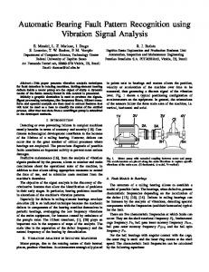
magnitude spectrum. The spectrum produced contains artifacts from noise, causing multiple peaks close together in frequency. These were reduced by smoothing the DFT magnitude spectrum using piecewise least-squares cubic curve fitting over a sliding window of 30 frequency points, resulting in a set of local maxima for each time ti . Step 3: Connect peaks in the current frame B to those in the previous frame A. Denote the set of peaks in frame A by {(tA , f1 , a1 ), (tA , f2 , a2 ), . . . , (tA , fm , am )} and those in frame B by {(tB , g1 , b1 ), (tB , g2 , b2 ), . . . , (tB , gn , bn )}, where fi , gi are frequencies and ai , bi are corresponding amplitudes. To determine which peak from frame B (if any) should be connected to (tA , fi , ai ) from frame A, find the nearest neighbor of (tB , fi , ai ) (in frequency) in frame B; call it (tB , gj , bj ). If the nearest neighbor to (tB , gj , bj ) in frame A is (tA , fi , ai ), then the two peaks should be connected. Otherwise, the track through (tA , fi , ai ) ends at (tA , fi , ai ). This particular algorithm for connecting peaks from consecutive frames was used by McAulay and Quatieri13 for speech analysis and a slightly modified version of this algorithm was used by Serra and Smith14 for analyzing the sounds produced by musical instruments. Repeat steps 1, 2, and 3 until there are no more frames left. Note that this process cannot connect tracks which cross, as could arise from two birds simultaneously vocalizing or two syringes within the same bird. The method is sufficient for the purposes of this paper, which deals with single vocalizations with non-crossing tracks. Step 4: Remove short and weak tracks in a “pruning” process: all tracks shorter than a user-specified duration δt and all but a user-specified percentage µ of the strongest tracks are removed. Track T1 is defined to be stronger than track T2 if the maximum amplitude in track T1 is greater than that in track T2 . Figure 1 a-c shows the three steps of preprocessing: spectrogram, raw track extraction, and automatic track pruning using δt = 0.1 sec, µ = 100% (in general, µ = 50% was used iteratively 7

(a)

(b)

(c)

(d)

FIG. 1. Preprocessing and hand-pruning for training, blue jay example: (a) spectrogram (Step 1), (b) after generation (Step 3) and (c) after pruning (Step 4). (d) Hand pruning in training.

to reduce labor of computing training sets). For recognition, δt = 0.04 and µ = 100% were used.

C. Segment calculation A track can be further approximated by a continuous piecewise linear function composed of line segments of alternating slope sign. It was necessary to first eliminate short segments that were induced by noise; the remaining linear pieces are called 8

track segments. The following algorithm was used with duration threshold βt = 0.02 seconds and frequency threshold βf = 20 Hz. Step 1: Smooth the track using least squares piecewise cubic curve fitting with a window size of 20 spectrogram frames and a step size of 5 frames. The resulting curve fit is continuously differentiable because the initial slope of the cubic curve in each window is constrained to equal the final slope of the cubic curve in the previous window. The curve fit in the first window is a line so that there are two degrees of freedom for the curve fit in each window. Step 2: From the saved cubic polynomial parameter sets for each track, calculate the local extrema (tk , fk ) over the track. Step 3: Mark extrema (tk+1 , fk+1 ) for deletion if |tk+1 −tk | < βt and |fk+1 −fk | < βf . Endpoint extrema are not removed. Step 4: After deleting and renumbering, further mark extrema (tk , fk ) for deletion if fk − fk−1 and fk+1 − fk have the same sign. Step 5: Form a piecewise linear approximation of the track by joining the remaining neighboring extrema with straight lines, retaining durations τk = tk+1 − tk and slopes δk = (fk+1 − fk )/τk .

III. TRAINING A. Harmonic structure Training is an abstraction of the information captured in the spectrograms for each vocalization type, and results primarily in a statistical model for each harmonic. Assume K instances of vocalization type V are selected as a training set. For each instance i of V a track set Ti is derived from Step 4 above. The K track sets Ti are analyzed by hand to identify H harmonics particular to V , including possibly a track 9

corresponding to the harmonic fundamental frequency. Once identified, each Ti is further pruned by hand to eliminate all tracks not consistent with the harmonics for V , resulting in track sets T i containing ni ≤ H valid tracks (see figure 1(d)). The model for V is created from these K track sets. For the four species of interest, the harmonic structure consisted of harmonics 0 through 9 for blue jay, 0 through 5 for herring gull, 0 through 7 for Canada goose, and harmonic 0 for American crow.

B. Descriptor sequence Certain birds have highly repetitive segment slope signs in the spectrograms of their vocalizations, such as the herring gull and the Canada goose. For these species, a visual analysis is done to identify the descriptor sequence: an alternating sequence of positively and negatively sloped segments. The descriptor sequence is defined by the sign s of the first segment and the total number of segments L and is used to correlate segments across harmonics. For other species (e.g. blue jay and American crow) a predictable sequence of slopes does not exist in the data analyzed.

C. The feature vectors The feature vectors for each vocalization class were determined by careful analysis of the track sets derived for training. For different species, different feature sets were required to obtain reasonably good classification results. A single track gives rise to two classes of features: track-derived features vA and segment-derived features vB ; these are used to form feature vectors v = (vA , vB ) for each species. A signal-to-noise ratio (SNR) η is also derived from the track and used for thresholding purposes during recognition. In the following let T be a track set, 10

and T ∈ T be a track.

1. Herring gull and Canada goose A. Let vA = (fˇ, fˆ, f¯, τ, A), where fˇ = minimum track frequency; fˆ = maximum track frequency; f¯ = mean track frequency; τ = track time length; A = track maximum amplitude normalized by track set maximum amplitude. The track SNR η is computed under the assumption that harmonic signal energy is sparse in the spectrogram representation, allowing for a good estimate of noise level using a median filter. For each frame time a coarse grid is formed at integer multiples of frequency interval size Wf . The noise level in the grid interval from l × Wf to (l + 1) × Wf , where l is a nonnegative integer, is estimated by the median value of all spectrogram points in that interval. The ratio η is computed by dividing the track maximum amplitude by the noise level from the grid intervals containing the frequency (fˆ + fˇ)/2 averaged over all the track time frames. Interval size Wf = 500 Hz was used providing roughly twelve 43 Hz bins, adequate for the median filter assuming harmonic tracks occupy three or fewer bins. B. Herring gull and Canada goose each possess a descriptor sequence S. For herring gull S = (−, 1), i.e. the sequence is one negatively sloped segment, and vB = (τ1 , δ1 ); for Canada goose S = (+, 2), i.e. a positively sloped segment followed by a negatively sloped segment, and vB = (τl , δl , τ2 , δ2 ). Here τi and δi are the segment duration and slope corresponding to segment i in the descriptor sequence. The tracks in T can contain more segments than the length of the descriptor sequence; only the duration and slope of the longest matching segment(s) to the descriptor sequence are retained in vB . 11

2. Blue jay A. The track-derived feature vector vA = (fˇ, fˆ, f¯, τ, A) is the same as for herring gull and Canada goose. B. For blue jay, segment slope sign is not consistent, and a descriptor sequence was ˇ δ, ˆ δ) ¯ where δˇ = minimum segment slope; δˆ = maximum not identified. Let vB = (δ, segment slope; and δ¯ = median segment slope.

3. American crow Based on the data analysis, crow tracks can be qualitatively described as oscillations superimposed on a concave curve, with many local extrema. This makes segmentation difficult and the American crow model uses only track-derived features. The main issue is capturing the concavity in a robust way. Critical to this is finding a local frequency maximum which is not at a track endpoint. Of the three greatest such maxima choose the one closest to the track time midpoint. If it exists, call this point (tC , fˆC ). Let (tL , fˇL ) be the absolute minimum frequency track point furthest to the left of t = tC , and (tR , fˇR ) be the minimum such point furthest to the right. Let ρ = (tC −tL )/(tR −tC ) (a skewness measure), ∆fL = fˆC − fˇL , and ∆fR = fˆC − fˇR . The American crow feature vector is then vA = (fˇL , fˆC , fˇR , ρ, ∆fL , ∆fR , τ ), where τ is duration. The signal-to-noise ratio η is computed as above.

D. Statistical model The tracks used to derive features capture the harmonic structure for the vocalization type. In general there will be Kh ≤ K tracks for harmonic h in the training data for vocalization V , as not all instances will contain all the harmonics due to 12

vocalization variability. Each such track results in a feature vector vi , according to species type, and an SNR ηi . Feature statistics are estimated by computing the mean v¯h and the covariance matrix Sh of the features over the Kh tracks for each harmonic h, resulting in a total of H mean-vector and covariance-matrix pairs (where H is the number of harmonics in the model.) Denote the Mahalanobis15 distance between feature vector v and feature vector mean v¯ by Dh (v). For each harmonic h compute the maximum such distance, and the minimum SNR, in the training set:

ˆ h = maxKh Dh (vi ) D i=1

(2)

h ηˇh = minK i=1 ηi .

(3)

To summarize, each vocalization model consists of some number of harmonics, and a descriptor sequence (which might be null). Each harmonic is described by a ˆ h , and an SNR threshold Mahalanobis distance function Dh (·), a distance threshold D ηˇh . In matching test vocalization harmonics to a particular model, the test SNR ˆ h for h. η must satisfy η > ηˇh , and the features must fall within the distance D For each species, some minimum number of such harmonic matches must occur for classification to occur. These numbers are any 3 out of 6 for herring gull, any 4 out of 10 for blue jay, harmonic 1 and at least one other out of 8 for Canada goose (since harmonic 1 occurred in every example in the training set), and 1 out of 1 for American crow. The numbers of required harmonics for the blue jay and herring gull were selected to eliminate false positives. When only three harmonics for blue jay or two harmonics for herring gull are required, false positives occur in the test data of other bird vocalizations. 13

IV. RECOGNITION

Recognition is accomplished in three steps: transformation of the input recording into a track file using the FTE algorithm, extraction of track sets from it that represent possible harmonic sounds, and comparison of each extracted set with the previously determined bird vocalization models.

A. Track set extraction

Track set extraction is done using two operations: an overlap criterion algorithm called find feasible sets (FFS) followed by a harmonic criterion algorithm called find maximal subsets (FMS); see figure 2.

1. Find feasible sets

Denote by T = {T1 , . . . , TN } the track set resulting from an input recording of arbitrary length. For each track Ti ∈ T form the corresponding accreted set Ai ⊂ T where Tj ∈ Ai if Tj overlaps Ti sufficiently in time, i.e. time-overlap is greater than δt , where δt is the minimum allowed track length as set in track pruning. The accreted set Ai contains all tracks potentially harmonically related to track Ti plus others due to noise, other vocalizations, and interfering signals. Each track is assumed to belong to at most one vocalization. A set function E, that maps pairs of track sets into new pairs, is used to obtain track sets A0i ⊂ Ai such that ∪i A0i = T and A0i ∩ A0j = ∅, for 14

FIG. 2. Image of all tracks in a track set of consecutive goose vocalizations, followed by image of the five feasible sets capturing the vocalizations, followed by the image of the six maximal subsets calculated from the feasible sets. Note that FMS splits feasible set 4 into the two maximal subsets maximal subset 4 and maximal subset 5.

all i, j. The function, called pair erosion, is defined by:

E(Ai , Aj ) =

   (Ai − Ai ∩ Aj , Aj )        for I(Ai , Aj ) < 0   (Ai , Aj − Ai ∩ Aj )        for I(Ai , Aj ) ≥ 0. 15

(4)

Here I(Ai , Aj ) is a measure of the importance of (accreted) track set Ai relative to track set Aj , defined by:

I(Ai , Aj ) =

A˜i Ni + Nj A˜j

! −

Nj A˜j + Ni A˜i

! (5)

where Ni is the number of tracks in Ai and A˜i is the average of the Ni track maximum amplitudes. If I(Ai , Aj ) > 0 then we say Ai is more important than Aj . The scoring function I can be used to establish an order relation on a set of track sets. Pair erosion is the removal of duplicate tracks from the less important track set. It is applied to each pair of accreted sets using the mapping (Ai , Aj ) → E(Ai , Aj ) until the resulting sets are pairwise disjoint. The remaining sets are called feasible sets. Some of the feasible sets will be empty; these are discarded. Although E is not quite symmetric, it is unlikely for two sets to have equal importance due to the floating point values used in its computation. More significantly it is possible for the feasible sets to depend on the order of the application of erosion. The time order imposed by the start of the earliest track in an accreted set was used here; this is consistent with the real-time flavor of the algorithm. Finally note that equal weighting is given to the terms Ni /Nj compared to A˜i /A˜j ; deeper investigation might reveal that this is not optimal.

2. Find maximal sets The algorithm find maximal sets (FMS) is then applied iteratively to each feasible set. It uses the harmonic correlation between two tracks to determine whether or not the tracks are related. Two tracks are harmonically correlated when the frequency ratios on the overlapping portions are nearly constant. A measure of this is the 16

function harmonic relate defined by: M

1 X |¯ r − ri |. H(Tj , Tk ) = M r¯ i=1

(6)

Here M is the number of pairs of track points (ti , fi , Ai ) and (ti , gi , Bi ) in the overlapping portions of the two tracks Tj and Tk . To make H symmetric, Tj , Tk are ordered P so that f¯i < g¯i . Then ri = gi /fi and r¯ = M i=1 ri /M . Let Ai , i = 0, 1, . . . be a track set with A0 a nonempty feasible set. For each track Tj in Ai , compute the harmonic accreted set Hj containing all tracks Tk such that H(Tj , Tk ) < , where  > 0 is a user specified threshold value; for this work  = .01. After ordering by importance, the most important harmonic accreted set is relabeled Hi , and we derive an eroded feasible set Ai+1 = Ai − Hi . The process is iterated until the resulting eroded set is empty, yielding the maximal subsets Hk , k = 0, . . . , n. For an isolated vocalization, FMS generally produces one large maximal set H0 and several small ones consisting of noise products; for coincident vocalizations it can separate the corresponding track sets.

B. Comparing extracted sets with the model To summarize, each input recording for recognition is converted into a track set using FTE, then partitioned in time into feasible sets, which are then partitioned in frequency into harmonically related maximal track sets. Each maximal set Hk is compared with the model of each species vocalization by comparing the tracks in it to the harmonic models in the vocalization model. If the track feature vector falls within the Mahalanobis distance of the submodel for that harmonic track it is called a harmonic match. If the set contains sufficiently many harmonic matches (see above), the recognizer declares the set Hk an occurrence of the vocalization. 17

C. Examples of recognition of target species The method just described was applied to blue jays, herring gulls and Canada geese. Track set extraction was not needed for American crows since the vocalization model contains only one track. Both rejection and detection performance were measured. Two test data sets were used, one collected by the authors containing the target and other species, and one collected by Robert Benson containing non-target species. Benson’s data set was used purely to test the ability of the recognition algorithm to reject sounds other than the target vocalization type. Ten species (including the four target species) were selected from our data set. The six other species in our data set were northern cardinal (Cardinalis cardinalis), fish crow (Corvus ossifragus), house sparrow (Passer domesticus), mallard (Anas platyrhynchos), white-breasted nuthatch (Sitta carolinensis), and European starling (Sturnus vulgaris); these recordings were also used to test rejection performance of the algorithm. Ten species were also selected from Benson’s data set: barn swallow (Hirundo rustica), Carolina wren (Thryothorus ludovicianus), eastern meadowlark (Sturnella magna), indigo bunting (Passerina cyanea), painted bunting (Passerina ciris), pine warbler (Dendroica pinus), red-winged blackbird (Agelaius phoeniceus), savannah sparrow (Passerculus sandwichensis), scissor-tailed flycatcher (Tyrannus forficatus), tufted titmouse (Baeolophus bicolor ). Table III lists the exact number of vocalizations in the recordings of the target species and the approximate number of vocalizations in the recordings of the other 16 species.

1. Blue jay The training set consisted of 64 hand-pruned track files corresponding to 64 blue jay vocalizations from 20 short recordings, recorded in summer, all from the same 18

Species

# of vocalizations

American crow

52

blue jay

45

Canada goose

45

herring gull

132

northern cardinal

4

fish crow

38

house sparrow

47

mallard

45

nuthatch

15

European starling

30

barn swallow

> 200

Carolina wren

> 150

eastern meadowlark

> 90

indigo bunting

> 90

painted bunting

> 250

pine warbler

> 40

red-winged blackbird

> 100

savannah sparrow

> 100

scissor-tailed flycatcher

> 130

tufted titmouse

> 300

TABLE III. Test data

19

Species

# vocalizations

# correctly identified

blue jay

45

37

herring gull

16

15

Canada goose

45

37

American crow

52

36

TABLE IV. Recognition results

individual. The test set consisted of 45 vocalizations, 19 of from the same individual as the training set and 26 from several other blue jays recorded at a nearby location in winter. The principal difficulties observed for blue jay calls were that they became chaotic, resulting in broken and irregular tracks at vocalization end, and the overall slope characteristics of the call tracks varied from call to call, resulting in a null descriptor sequence. Thirty-seven out of 45 blue jay vocalizations were correctly identified (see Table IV); no false positives resulted from other species.

2. Herring gull Herring gulls vocalize with a variety of syllables, each requiring its own feature model. The syllable types are distinguished from each other by the number and length of the segments, the descriptor sequence, and the vocalization fundamental frequency. In the recording database, there is one syllable that occurs 31 times, and several others that occur 7 or fewer times each. A model for the most common syllable was made using 15 of the 31 processed track files for a training set. Since the 20

syllable is always down-sloping in frequency, its descriptor sequence is (−, 1). Using ˆ h determined during training, applied to the recordings containing the the values of D 16 remaining syllables, 11 were correctly recognized. This low rate is likely due to the limited amount of training data which produced a Mahalanobis distance threshold less than 14 on each harmonic, as compared to 40 for blue jay and 38 for Canada goose. Using a value of 40 for each harmonic resulted in 15 out 16 correctly identified with no false positives, as shown in Table IV. Increasing this value further, there were no false positives up to a distance value of 75 and all 16 vocalizations were correctly recognized. At a value of 100, there were false positives for eastern meadowlark and other gull vocalization syllables.

3. Canada goose Canada geese have one primary vocalization type and several secondary vocalizations. This work focused on recognizing only the primary vocalization type. The frequency curve of the primary vocalization type is concave down with an up-sloping part followed by a down-sloping part (so the descriptor sequence is (+, 2)). Less commonly, Canada geese make a similar vocalization with no up-sloping initial part, as well as hissing and grunting sounds. The training data used to make the model for the primary goose vocalization type was collected from a large flock of geese at Sunken Meadow State Park and the data (a 1 minute long recording of a flock) used to test recognition performance of this vocalization type was collected at the park later on the same day. Many different birds were vocalizing in both the training and test set, and a fairly wide range (500-850 Hz) of vocalization fundamental frequencies are present. The test set contained 45 primary goose vocalizations, of which 37 were correctly recognized by the algorithm. The recognizer was again applied to the 21

Species

# of false positives

type

Amer. crow

3

Canada goose

Canada goose

1

Amer. crow

TABLE V. Rejection results

data set of other species, with a false positive occurring in one of the American crow recordings (as shown in table V).

4. American crow For American crows, recognition is carried out track by track, and track set extraction is not done. Moreover, the crow model is considerably different from the other three species. In particular, the Mahalanobis distance criterion produced a large number of false positives, and an alternative distance function was used. Using a training set containing 40 crow vocalizations and a test set of 52 crow vocalizations, the results in Tables IV and V were obtained. These results are included here for completeness. The measure used was binary: the maximum and minimum values for each feature in the crow training set were used to determine a feature range. A track matched the harmonic model if each feature fell within the range.

V. CONCLUSION This paper demonstrates an algorithm for harmonic frequency track extraction and its application to classification of birds by vocalization analysis. First, a frequency 22

track representation of the sound segment is calculated, resulting in a track file. Second, the track file is separated into track sets (feasible sets) calculated using an overlap criterion. Third, each feasible set is divided into disjoint harmonically related subsets (maximal sets). Finally, each maximal set is compared with the vocalization models. The performance of the recognizer was fair (crow) to very good (blue jay) on target species, and excellent on false positives. Improved recognition performance can likely be obtained by more refined feature sets and more extensive data sets. The only false positives that occurred were when crow and goose were identified as one another. If more species were considered, it is possible that more features would be needed in order to achieve this level of performance in rejecting false positives.

Acknowledgments This work was funded by the Air Force Office of Scientific Research, the Research Foundation of Stony Brook University and Advanced Acoustic Concepts, Inc. The authors would like to thank Willard Larkin of AFOSR for suggesting the application of acoustic processing to bird-strike avoidance; to James Glimm, Bruce Stewart, and Robert Benson for helpful comments and discussions, and to the reviewers for their constructive criticisms.

References 1

E. C. Cleary, R. A. Dolbeer, and S. E. Wright, “Wildlife strikes to civil aircraft in the United States: 1990-2005”, Technical Report 12, Federal Aviation Administration (2006), 362 pp. 23

2

R. P. DeFusco, “A bird avoidance model for the US Air Force”, USAFA Discovery 98, 1–2 (1998).

3

R. Shade, “Auditory cortex analysis phase 2 proposal”, Technical Report, Advanced Acoustic Concepts (2004), 42 pp.

4

J. A. Kogan and D. Margoliash, “Automated recognition of bird song elements from continuous recordings using dynamic time warping and hidden Markov models: A comparative study”, J. Acoust. Soc. Am. 103, 2185–2196 (1998).

5

A. H¨arm¨a and P. Somervuo, “Classification of the harmonic structure in bird vocalization”, in IEEE ICASSP (2004), pp. 17-21.

6

S. Fagerlund, “Automatic recognition of bird species by their sounds”, Master’s thesis, Helsinki University of Technology (2004), 65 pp.

7

Z. Chen and R. C. Maher, “Semi-automatic classification of bird vocalizations using spectral peak tracks”, J. Acoust. Soc. Am. 120, 2974–2984 (2006).

8

S. E. Anderson, A. S. Dave and D. Margoliash, “Template-based automatic recognition of birdsong syllables from continuous recordings”, J. Acoust. Soc. Am. 100, 1209–1219 (1996).

9

J. R. Buck and P. L. Tyack, “Quantitative measure of similarity for Tursiops truncatus signature whistles”, J. Acoust. Soc. Am. 94, 2497–2506 (1993).

10

D. K. Mellinger and C. W. Clark, “Recognizing transient low-frequency whale sounds by spectrogram correlation”, J. Acoust. Soc. Am. 107, 3518–3529 (2000).

11

L. R. Rabiner and B. Juang, Fundamentals of Speech Recognition (Prentice Hall) (1993).

12

K. M. Fristrup and W. A. Watkins, “Marine animal sound classification”, Technical Report 13, Woods Hole Oceanographic Institution (1994), 32 pp.

13

R. J. McAulay and T. F. Quatieri, “Speech analysis/synthesis based on a sinusoidal representation”, IEEE Trans ASSP 34, 744–754 (1986). 24

14

X. Serra and J. Smith, “Spectral modeling synthesis”, Computer Music Journal 14, 12–24 (1990).

15

K. V. Mardia , J. T. Kent and J. M. Bibby, Multivariate Analysis (Academic Press) (2000).

25