Automatic Recognition of Landforms on Mars Using Terrain Segmentation and Classification Tomasz F. Stepinski1 Soumya Ghosh2 and Ricardo Vilalta2 1
2
Lunar and Planetary Institute, Houston, TX 77058, USA,
[email protected] Department of Computer Science, University of Houston, Houston, TX 77204, USA,
[email protected] [email protected]
Abstract. Mars probes send back to Earth enormous amount of data. Automating the analysis of this data and its interpretation represents a challenging test of significant benefit to the domain of planetary science. In this study, we propose combining terrain segmentation and classification to interpret Martian topography data and to identify constituent landforms of the Martian landscape. Our approach uses unsupervised segmentation to divide a landscape into a number of spatially extended but topographically homogeneous objects. Each object is assigned a 12 dimensional feature vector consisting of terrain attributes and neighborhood properties. The objects are classified, based on their feature vectors, into predetermined landform classes. We have applied our technique to the Tisia Valles test site on Mars. Support Vector Machines produced the most accurate results (84.6% mean accuracy) in the classification of topographic objects. An immediate application of our algorithm lies in the automatic detection and characterization of craters on Mars.
1
Introduction
Landforms in Mars are characterized using imagery and altimetry data. Impact craters are among the most studied landforms on Mars. Their importance stems from the amount of information that a detailed analysis of their number and morphology can produce. Visual inspection of imagery data by domain experts has produced a number of catalogs [3, 22] that list crater locations and diameters. Automated algorithms for crater detection from imagery data exist [14, 16, 8, 27, 28], but none has been deemed adequately accurate to be employed in a scientific study because of poor accuracy (mainly because of false identifications). In this paper we develop a methodology for automatic identification of landforms on Mars using altimetry (topographic) data. Our goal is to identify craters’ floors and their corresponding walls from other landforms. The distinction between floors and walls is important for subsequent calculation of crater geometry [20]. An accurate knowledge of the geometry for a large database of Martian craters would enable studies with a number of outstanding issues and potential discoveries, such as the nature of degradation processes [24], regional variations in geologic material [10], and distribution of subsurface volatiles [11], leading to
a much better understanding of the composition of the planet’s surface and its past climate. Our strategy departs significantly from that employed in [25, 7]. First, we move away from a pixel-based analysis and adopt an object-based analysis [2], which is more appropriate for spatially extended data. Object-based analysis originated in applications of image analysis of remotely sensed data, where an image is segmented into a number of image objects –areas of spectral and/or textural homogeneity. Our approach is based on extending the notion of objects from images to topographic data, and our first task is to segment a given site into topography objects –areas of topographic homogeneity. Second, we move away from clustering (unsupervised learning) and adopt classification (supervised learning) by assigning landform class label to each object. This change assures that the resultant classification corresponds to recognizable landforms. Classification is feasible because the classified units are now objects instead of pixels. Objects have clear topographic meaning and are more suitable than individual pixels for manual labeling. The number of units to be handled is drastically reduced making the classification process viable. Finally, objects are the source of additional information, such as their size, aggregative statistics, and neighborhood information which are used as extra features for classification. The novelty of our study can be summarized as follows: 1) the automatic segmentation of a terrain into constituent objects is a new concept in the context of terrain analysis; it has applications in both planetary and terrestrial geomorphology. The methodology creates a spatial database otherwise inaccessible to terrain analysis; 2) using classification algorithms to aggregate segmentation objects into larger, physically relevant structures, is a new concept readily available for data analysis techniques (particularly spatial data mining).
2
Background Information
There are currently four space probes on orbits around Mars remotely collecting data about its surface. They generate a deluge of data, but only a small fraction of this data can be interpreted because analysis is performed manually at high “cost” by domain experts. Automation is the only practical solution to the challenge behind processing a significant portion of the –ever increasing– volume of Martian data. Martian craters, despite having deceptively simple circular appearance, present a formidable challenge for a pattern recognition algorithm. Some craters are degraded by erosion and are barely distinguishable from their background. In a heavily cratered terrain, where an automated detection is most desirable, there is a significant degree of crater overlapping. Finally, crater sizes differ by orders of magnitude. Image-based detection techniques face additional difficulties as the “visibility” of an impact crater depends on the image quality. Other landforms on Mars, as for example valleys, also present challenges for automatic recognition [19].
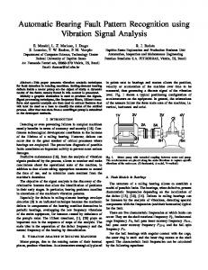
Fig. 1. A perspective view of the Tisia Valles landscape rendered using the DEM. The vertical dimension is exaggerated 10 times, and the north is to the left.
Recently, landform detection algorithms have begun to use topography data as an alternative to images. Mars is the only planet besides the Earth for which global elevation model (DEM) data is available [23]. A DEM is a raster dataset where each pixel is assigned an elevation value. In [25, 7] Martian sites are divided into mutually exclusive and exhausting landform categories on the grounds of similarity between pixel-based vectors of terrain attributes. In both studies, landform categories are the result of unsupervised clustering of these vectors, but whereas [25] employs a probabilistic algorithm working under a Bayesian framework, [7] employs a self-organizing map [17]. In principle, these methods avoid the issue of crater identification by automatically categorizing all landforms (including craters) in a given site. The clustering-based division of a site into constituent landforms has the advantage of being an unsupervised, low “cost” process, but it also suffers from the lack of direct correspondence between clusters and generally recognizable landforms. A significant manual post-classification processing is necessary to interpret all results. In addition, some landforms of interest (like, for example, craters’ walls) are poorly represented by any single cluster, or even group of clusters.
3
Study Site and Terrain Attributes
Fig. 1. shows a DEM-derived shaded relief of our Tisia Valles test site centered at 46.13o E, 11.83o S. The DEM has a resolution of 500 meters and its dimensions
are N = 385 rows and M = 424 columns. This is a challenging site for landform identification. In a relatively small area many different crater morphologies are present: fresh deep craters with intact walls; old, degraded craters with various degrees of wall erosion; conjoined craters with various degrees of overlap. All these different types of craters are present in a range of sizes. In addition, the site is crossed from south-west to north-east by a broad valley with escarpments on both sites. The valley floor is further sculptured. Smaller scale valleys are present at inter-crater highlands. The same site was previously used in [25]. The DEM carries information about terrain elevation, z(x, y) at the location of each pixel. Terrain attributes are additional raster datasets calculated from the DEM. In this study we use three terrain attributes: slope, curvature, and flood. The slope, s(x, y), is the rate of maximum change of z on the Moore neighborhood1 of a pixel located at (x, y). The (profile) curvature, κ(x, y), measures the change of slope angle and is also calculated using the values of z on the Moore neighborhood of a pixel (κ > 0 correspond to convex topography, whereas κ < 0 correspond to concave topography). The flood, f (x, y), is a binary variable; pixels located inside topographic basins have f (x, y) = 1, and all other pixels have f (x, y) = 0. A vector, V(x, y) = {z, s, κ, f }(x, y) describes the topography of the landscape at the level of an individual pixel. We refer to the (N − 2) × (M − 2) array of vectors V as the landscape. The landscape is smaller than a DEM because the DEM’s edge is eliminated (by removing the two rows and two columns lying on the array boundaries) due to calculations of derivatives using the Moore neighborhood.
4
Segmentation
In the context of image analysis the term segmentation refers to a process of dividing an image into smaller regions having homogeneous color, texture, or both. We have observed that the notion of segmentation can be applied not only to multi-band images, but to all spatially extended datasets including multiattribute landscapes. A variety of techniques [1, 4, 13, 21] have been proposed to implement image segmentation, and all of them can be, in principle, easily extended to landscape segmentation. In [15] a computationally simple homogeneity index H was proposed, and in [9] this index was combined with the watershed transform [26] for fast, unsupervised segmentation of multi-band images. In this paper we utilize this method for segmentation of multi-attribute landscapes. The homogeneity measure H is calculated using a square window of width 2K + 1 (where K is user-defined). Consider a focal pixel (xc , yc ) having an attribute (for example, an elevation z) z(xc , yc ). For every pixel in a window we calculate a “separation” vector di = (xi − xc , yi − yc ). From the separation vector we construct a “gradient” vector, gi = (z(xi , yi ) − z(xc , yc )) 1
di kdi k
(1)
The Moore neighborhood around a focus pixel (x0 , y0 ) is a square-shaped area defined by {(x, y) : |x − x0 | ≤ 1, |y − y0 | ≤ 1}.
Fig. 2. Segmentation of Tisia Valles landscape into 2631 topographically homogeneous objects.
and we use gradient vectors calculated for all pixels in a window to calculate the homogeneity measure H, ° ° °(2K+1)2 ° ° X ° H=° gi ° (2) ° ° ° i=1 ° A pixel located in the region that is homogeneous with respect to z has a small value of H. On the other hand, a pixel located near a boundary between two regions characterized by different values of z has a large value of H. A raster constructed by calculating the values of H for all pixels in the landscape can be interpreted as a gray scale image and is refered to as the Himage. We denote the H-image by H. The white areas on H represent boundaries of homogeneous regions, whereas the dark areas represent the actual regions. The extension of the H-image concept to multiple attributes is straightforward. Let’s say that we want to calculate the H of a landscape on the basis of slope, curvature, and flood attributes. For each pixel we calculate the three individual H values separately and combine them to obtain the overall value of H at that pixel: q H = ws Hs 2 + wκ Hκ 2 + wf Hf 2 (3) where ws , wκ , and wf are weights introduced to offset different numerical ranges of the attributes.
We have segmented the Tisia Valles landscape using three attributes, s, κ and f . Note that we have opted not to use z as a segmentation attribute because no landforms are characterized by their elevations. We use the H-image technique with K = 2 to obtain Hs , Hκ , and Hf . Individual H-images are subject to thresholding, ½ Hk (x, y) = Hk (x, y) if Hk (x, y) > Tk Hk (x, y) = (4) Hk (x, y) = 0 otherwise where k = s, κ, f , and Tk is an appropriate threshold value introduced to prevent oversegmentation caused by high sensitivity to noise. The thresholded H-images are combined using formula (3) and the combined H-image is segmented using the watershed transform. This procedure segments the site into 2631 topographic objects as shown in Fig. 2. Each object is topographically homogeneous. Note that the number of objects is two orders of magnitude smaller than 161,626 pixels constituting the DEM. The objects are small where topography changes on a small spatial scale, like, for example, on the walls of the craters, or at the escarpments. On the other hand, objects are large when changes occur on only a large spatial scale, like, for example in the inter-crater plain, or on the floors of large craters. The largest object has 15,106 pixels, and the 13 largest objects occupy 75% of the site’s area. For each object, i = 1, . . . , 2631, we calculate the mean values, s¯i , κ¯i , f¯i , and standard deviation values, σis , σiκ , σif , from its constituent pixels. We refer to s¯i , κ¯i , and f¯i simply as slope, curvature, and flood of an object. Objects making up craters’ walls and objects constituting escarpments not associated with craters have similar topographic attributes but are located in different spatial contexts. The object’s neighborhood properties provide some information about that context. Ideally, we would like to know classes of object’s neighbors, but such information is not available prior to classification. However, a preliminary categorization of objects is possible on the basis of their values of s¯i , κ¯i , f¯i . We divide all objects into three categories (low, medium, and high) on the basis of their slope values. Such categorization is used to calculate a neighborhood property of an object i, {as1 , as2 , as3 }i , where asj , j = 1, 2, 3, is the percentage of the object boundary adjacent to neighbors belonging to slope category j. Similar neighborhood properties, {aκ1 , aκ2 , aκ3 }i , {af1 , af2 , af3 }i , are calculated on the basis of curvature and flood values, yielding a total of nine attributes corresponding to the spatial context of objects.
5
Classification
We classify topographic objects into six landform classes with clear physical meaning. Class 1 consists of inter-crater plains, a flat terrain that in most cases is homogeneous on relatively large spatial scale. Class 2 consists of craters’ floors, a flat terrain inside craters. Class 3 consists of convex craters’ walls, whereas class 4 consists of concave craters’ walls. Classes 5 and 6 consists of objects that are
located on convex and concave non-crater escarpments, respectively. We use the following 12-dimensional feature vector to characterize each segment, n o (5) u = s¯, κ ¯ , f¯, as1 , as2 , as3 , aκ1 , aκ2 , aκ3 , af1 , af2 , af3
Fig. 3. Training set of 517 labeled topographic objects, 10% gray indicates class 1, black indicates class 2, 20% gray indicates class 3, 80% gray indicates class 4, and 40% gray indicates classes 5 and 6.
We note that the object’s size, its elevation, and its σis , σiκ , σif values are not presently used as part of the feature vector. In general, objects’ sizes and elevations have proved to be poor indicators of their class as defined in this study. Inclusion of σis , σiκ , σif into the feature vector produces no improvement in classification. 5.1
Training Set
We have manually labeled 517 topographic objects to make up a training set. This set constitutes 20% of all objects and 29% of the site’s area. The location of training set objects is shown on Fig. 3. Due to the limitation of illustrating a site using gray scales, classes 5 and 6 are shown employing the same gray shade. The objects were selected for labeling on the basis of geographical coherence (see Fig. 3) but we have also made sure that all landform classes are represented in the training set.
To provide additional information regarding our training set, Table 1 (left side) shows for each class (each row), the number of objects in that class, the fraction of the training set’s total area covered by the objects in the class, and the values of the three physical features, s, κ, and f , averaged over objects in each class. The right side of Table 1 provides the same information but for all objects constituting the Tisia Valles site as divided into classes by using a classifier obtained using a Support Vector Machine. Table 1. Properties of topographic objects in six landform classes averaged over the training set (left) and the entire set (right). class object area s κ f object area s κ f count site % deg. ×103 count site % deg. ×103 517 objects in the training set All 2631 objects 1 89 54.0 0.99 -0.1 0.04 957 64.5 0.96 0.12 0.03 2 5 24.0 0.83 0.41 1.0 26 11.5 0.83 0.58 0.91 3 163 9.0 5.24 3.12 0.78 536 8.0 5.2 3.54 0.83 4 145 8.0 4.08 -3.78 0.08 674 10.0 4.11 -4.62 0.13 5 61 2.6 2.49 2.61 0.09 208 2.0 2.02 2.27 0.08 6 54 2.4 2.20 -2.01 0.0 230 4.0 1.78 -1.79 0.0
5.2
Classification results
Table 2 (left side) shows the result of invoking various learning algorithms on our training set. Each entry shows the average of 5 runs of 10-fold cross validation (numbers in parentheses represent standard deviations). All algorithms follow the implementation of the software package WEKA [29] using default parameters2 . An asterisk at the top right of a number implies the difference is significantly worse than the first algorithm (Support Vector Machine) at the p = 0.05 level assuming a two-tailed t-student distribution. Table 2 was produced to observe the inherent difficulty associated with differentiating between various Martian landforms. The advantage of relatively complex models over simpler ones points to the need for flexible decision boundaries. The apparent advantage of bagging over the decision tree points to some degree of variance [6]. The right side of Table 2 shows a confusion matrix obtained using the Support Vector Machine model. Overall, the exclusion errors (i.e., false negatives) are acceptable with the exception of class 6. A significant number of class 6 (concave escarpment) objects are classified as either class 4 (concave crater walls), as we could expect 2
SVM uses a cubic kernel with a complexity parameter of C = 1. Decision tree uses reduced error pruning with a confidence factor of 0.25 and a stopping criterion for splitting of size 2. Bagging uses bootstrap samples of size equal to the training set and average values over 10 trees. Neural network uses a learning rate of 0.3 and momentum of 0.2 with 500 epochs. k-nearest neighbor uses k = 5 and the KKDtree algorithm [5]. Bayesian Network builds a network using the K2 algorithm [12].
Table 2. (Left) Accuracy by averaging over 5 x 10-fold cross-validation for various learning algorithms. An asterisk at the top right of a number indicates a statistically significant degradation with respect to the first algorithm (Support Vector Machine). Numbers enclosed in parentheses represent standard deviations. (Right) Confusion matrix for the Support Vector Machine algorithm, exclusions (false negatives) are in the rows, erroneous inclusions (false positives) are in the columns.
Learning Algorithm
Accuracy Estimation Confusion Matrix 1 2 3 4 5 6 Support Vector Machine 84.61 (4.89) 85 0 1 0 3 0 Neural Network 81.71 (5.09) 0 4 1 0 0 0 Bagging 83.02 (5.30) 2 1 146 10 4 0 Decision Tree 81.01∗ (5.09) 7 1 8 119 0 10 Bayesian Network 79.42∗ (5.75) 3 0 4 0 54 0 Nearest Neighbor 78.77∗ (5.15) 13 0 0 11 1 29
from the local similarity between the two landforms, or as class 1 (inter-crater plains). The largest number of exclusions from class 4 are, as expected, picked up by class 6, but some are picked up by classes 1 and 3. Surprisingly, there is not much confusion between classes 5 and 3. This is probably due to the large difference between the values of the flood attribute in the two classes (see Table 1). The erroneous inclusion errors (i.e., false positives) show similar patterns. Interestingly, class 1 (a big inter-crater plain) suffers a small degree of erroneous inclusions from most other classes that, in general, are characterized by very different values of physical features. Using a decision function calculated on the basis of the Support Vector Machines model, we have classified all 2631 objects in the Tisia Valles site. The spatial illustration of this classification is shown on Fig. 4 and the numerical results of the classification are given in Table 1 (right side). The values of the three physical features averaged over objects belonging to the same class are very similar to corresponding values in the training set. This reassures us that the training set constitutes a representative sample of the entire site. Visual inspection of Fig. 4 indicates that classification successfully divided the landscape into its landforms. Large craters are perfectly delineated from the inter-crater plain, and most of the escarpment is also correctly identified. A more in depth examination reveals some inevitable shortcomings. The classifier does not identify the centers of small craters as floors (class 2). Technically, this is correct, because such craters are too small to have flat “floors,” but such omissions complicate the process of crater recognition. The smallest craters have centers represented by class 3 objects, which are surrounded by class 4 objects, too large to produce a correct representation of their walls. This is due to insufficient resolution of our segmentation. Finally, there are some limited problems
Fig. 4. Classification of all 2631 topographic objects, 10% gray indicates class 1, black indicates class 2, 20% gray indicates class 3, 80% gray indicates class 4, and 40% gray indicates classes 5 and 6.
in the correct delineation of small relief escarpments. Overall these shortcomings are minor; most of the complex landscape was correctly interpreted.
6
Conclusions and Future Work
The success of our method depends on two factors, the quality of segmentation and the choice of an appropriate feature vector. Martian terrain requires that the range of topography objects sizes span few orders of magnitude. Although our segmentation achieves this requirement, a larger range is necessary to resolve the smallest craters. Future work will have to address this issue. One possible solution is to avoid a single watershed threshold, and rather use an adaptive threshold with a value that is coupled to the spatial scale of the change in topography. Our segmentation process can also be viewed as the process of creating a spatial database of topography objects. In spatial data mining, objects are characterized by different types of information: non-spatial attributes, spatial attributes, spatial predicates, and spatial functions [18]. In this paper we have considered only physical features (corresponding to non-spatial attributes) and some neighborhood relations (corresponding to spatial attributes). Using just the physical features produced a 77.4% classification accuracy; this accuracy
increases to 84.6% when features based on neighborhood properties are also considered (using a Support Vector Machine). Future studies will employ spatial predicates and spatial functions to further increase our current predictive accuracy. Finally, we stress that the present classification allows for an automatic identification and characterization of large and medium craters. A study is underway to use our technique to calculate geometries of such craters on Sinai Planum and Hesperia Planum, two locations on Mars that, although similar, are expected to have systematic differences in crater morphologies [20]. Acknowledgements This work was supported by the National Science Foundation under Grants IIS0431130, IIS-448542, and IIS-0430208. A portion of this research was conducted at the Lunar and Planetary Institute, which is operated by the USRA under contract CAN-NCC5-679 with NASA. This is LPI Contribution No. 1301.
References 1. Adams, R. Bischof, L.: Seeded Region Growing. IEEE Trans. Pattern Analysis and Machine Intelligence. 16(6) (1994) 641–647 2. Baatz M., Sch¨ ape, A.: Multiresolution Segmentation - An Optimization Approach for High Quality Multi-Scale Image Segmentation. In: Strobl, J. et al. (eds.): Angewandte Geographische Infor-mationsverarbeitung XII. Wichmann, Heidelberg. (2000) 12-23 3. Barlow, N.G.: Crater Size-Distributions and a Revised Martian Relative Chronology. Icarus. 75(2) (1988) 285-305 4. Belongie, S., Carson, C., Greenspan, H. Malik, J.: Color- and Texture-based Image Segmentation Using EM and its Application to Content-based Image Retrieval. Proc. of Sixth IEEE Int. Conf. Comp. Vision. (1998) 675-682 5. Bentley J. L.: Multidimensional Binary Search Trees Used for Associative Searching. Communications of ACM, 18, (9), (1975), 509–517. 6. Breiman, L.: Bagging Predictors. Machine Learning, 24, (1996) 123–140. 7. Bue, B.D., Stepinski, T.F.: Automated classification of Landforms on Mars. Computers & Geoscience. 32(5) (2006) 604-614 8. Burl, M.C., Stough, T., Colwell, W., Bierhaus, E.B., Merline, W.J.,Chapman, C.: Automated Detection of Craters and Other Geological Features. Proc. Int. Symposium on Artificial Intelligence, Robotics and Automation for Space, Montreal, Canada. (2001) 9. Chen, Q., Zhou, C., Luo, J., Ming, D.: Fast Segmentation of High-Resolution Satellite Images Using Watershed Transform Combined with an Efficient Region Merging Approach. Proc. 10th Int. Workshop Combinatorial Image Analysis. Lecture Notes in Computer Science, Vol 3322. Springer-Verlag, Berlin Heidelberg New York (2004) 621–630 10. Cintala, M.J., Head, J.W., Mutch, T.A.: Martian Crater Depth/Diameter Relationship: Comparison with the Moon and Mercury. Proc. Lunar Sci. Conf. 7 (1976) 3375-3587
11. Cintala, M.J., Mouginis-Mark, P.J.: Martian Fresh Crater Depth: More Evidence for Subsurface Volatiles. Geophys. Res. Lett. 7 (1980) 329-332 12. Cooper, G.F., Herskovits, E.: A Bayesian Method for the Induction of Probabilistic Networks from Data. Machine Learning 9(4) (1992) 309–347. 13. Deng, Y., Manjunath, B.S.: Unsupervised Segmentation of Color-Texture Regions in Images and Video. IEEE Trans. Pattern Analysis and Machine Intelligence. 23(8) (2001) 800–810 14. Honda, R., Iijima, Y., Konishi, O.: Mining of Topographic Feature from Heterogeneous Imagery and Its Application to Lunar Craters. Progress in Discovery Science: Final Report of the Japanese Discovery Science Project, Springer-Verlag, Berlin Heidelberg New York (2002) p. 395 15. Jing, F., Li, M.J., Zhang, H.J., Zhang, B.: Unsupervised Image Segmentation Using Local Homogeneity Analysis. Proc. IEEE International Symposium on Circuits and Systems. (2003) II-456–II-459 16. Kim, J.R., Muller, J-P., van Gasselt, S., Morley, J.G., Neukum, G., and the HRSC Col Team: Automated Crater Detection, A New Tool for Mars Cartography and Chronology. Photogrammetric Engineering & Remote Sensing. 71(10) (2005) 1205-1217 17. Kohonen, T.: Self-Organizing Maps. Springer-Verlag, Berlin Heidelberg New York (1995) 18. Koperski, K., Han, J., Stefanovic, N.: An Efficient two-Step Method for Classification of Spatial Data. Proc. Eight Symp. Spatial Data Handling. (1998) 45-55 19. Molloy, I., Stepinski, T.F.: Automatic Mapping of Valley Networks on Mars. Submitted to Computers & Geoscience (2006) 20. Mouginis-Mark, P.J., Garbeil, H., Boyce, J.M., Ui, C.S.E., Baloga, S.M.: Geometry of Martian Impact Craters: First Results from an Iterative Software Package. J. Geophys. Res. 109 (2004) E08996 21. Nock, R., Nielsen, F.: Stochastic Region Merging. IEEE Trans. Pattern Analysis and Machine Intelligence. 26(11) (2004) 1452–1458 22. Rodionova, J.F., Dekchtyareva, K.I., Khramchikhin, A.A., Michael, G.G., Ajukov, S.V., Pugacheva, S.G., Shevchenko, V.V.: Morphological Catalogue Of The Craters Of Mars. ESA-ESTEC (2000) 23. Smith, D., Neumann, G., Arvidson, R.E., Guinness, E.A., Slavney, S.: Mars Global Surveyor Laser Altimeter Mission Experiment Gridded Data Record. NASA Planetary Data System, MGS-M-MOLA-5-MEGDR-L3-V1.0. (2003) 24. Soderblom, L.A., Condit, C.D. West, R.A., Herman, B.M., Kreidler, T.J.: Martian Planetwide Crater Distributions: Implications for Geologic History and Surface Processes. Icarus, 22 (1974) 239-263 25. Stepinski, T.F., Vilalta, R.: Digital Topography Models for Martian surfaces. IEEE Geoscience and Remote Sensing Letters. 2(3) (2005) 260-264 26. Vincent, L., Soille, P.: Watersheds in Digital Spaces: An Efficient Algorithm Based on Immersion Simulations. IEEE Trans. Pattern Analysis and Machine Intelligence. 13(6) (1991) 583–598 27. Vinogradova, T., Burl, M., Mjosness, E.: Training of a Crater Detection Algorithm for Mars Crater Imagery. Aerospace Conference Proc. 2002, IEEE. 7 (2002) 7-3201 - 7-3211 28. Wetzler, P.G., Enke, B., Merline, W.J., Chapman, C.R., Burl, M.C.: Learning to Detect Small Impact Craters. Seventh IEEE Workshops on Computer Vision (WACV/MOTION’05). 1 (2005) 178-184 29. Witten I. H., Frank E.: Data Mining: Practical Machine Learning Tools and Techniques with Java Implementations. Academic Press, London U.K. (2000).